Article

Application and Evaluation of a Deep Learning Architecture to Urban Tree Canopy Mapping

1
Department of Geography, University of Idaho, Moscow, ID 83844, USA
2
Department of Computer Science, University of Idaho, Idaho Falls, ID 83406, USA
*
Author to whom correspondence should be addressed.
Remote Sens. 2021, 13(9), 1749; https://doi.org/10.3390/rs13091749
Submission received: 3 April 2021 / Revised: 25 April 2021 / Accepted: 28 April 2021 / Published: 30 April 2021

Abstract

:
Urban forest is a dynamic urban ecosystem that provides critical benefits to urban residents and the environment. Accurate mapping of urban forest plays an important role in greenspace management. In this study, we apply a deep learning model, the U-net, to urban tree canopy mapping using high-resolution aerial photographs. We evaluate the feasibility and effectiveness of the U-net in tree canopy mapping through experiments at four spatial scales—16 cm, 32 cm, 50 cm, and 100 cm. The overall performance of all approaches is validated on the ISPRS Vaihingen 2D Semantic Labeling dataset using four quantitative metrics, Dice, Intersection over Union, Overall Accuracy, and Kappa Coefficient. Two evaluations are performed to assess the model performance. Experimental results show that the U-net with the 32-cm input images perform the best with an overall accuracy of 0.9914 and an Intersection over Union of 0.9638. The U-net achieves the state-of-the-art overall performance in comparison with object-based image analysis approach and other deep learning frameworks. The outstanding performance of the U-net indicates a possibility of applying it to urban tree segmentation at a wide range of spatial scales. The U-net accurately recognizes and delineates tree canopy for different land cover features and has great potential to be adopted as an effective tool for high-resolution land cover mapping.

1. Introduction

Urban forests are an integral part of urban ecosystems. They provide a broad spectrum of perceived benefits, such as improved air quality, lower surface and air temperatures, and reduced greenhouse gas emissions [1,2,3,4]. Additionally, urban trees can improve human mental health by adding aesthetic and recreational values to the urban environment [5,6,7]. The last decade has witnessed a dramatic decline of urban tree cover. From 2009 to 2014, there was an estimated 70,820 hectares of urban tree cover loss throughout the United States [8]. A better understanding of tree canopy cover is more important than ever for sustainable monitoring and management of urban forests.
Urban tree canopy, defined as the ground area covered by the layer of tree leaves, branches and stems [9], is among the most widely used indicators to understand urban forest pattern. Conventionally, field-based surveys are conducted to manually measure the area of urban vegetation [3,10,11]. The field-based surveys are mostly conducted by regional forestry departments and various research programs, and many of the field surveys are highly costly and labor intensive [12]. The availability of digital images and advances of remote sensing technologies provide unique opportunities for effective urban tree canopy mapping [13,14]. For instance, the Moderate Resolution Imaging Spectroradiometer–Vegetation Continuous Field (MODIS–VCF) product provides global coverage of percent tree canopy cover at a spatial resolution of 500 m [15]. This product is one of the most adopted vegetation map products to study global tree canopy trends and vegetation dynamics. Other satellite images such as the Landsat imagery [16] and the Satellite Pour l’ Observation de la Terre (SPOT) imagery are frequently used for studying tree canopy cover at local and regional scales [17,18,19,20]. Very high-resolution satellite images have increasingly been employed in forest management and mapping at meter and sub-meter levels. The National Agriculture Imagery Program (NAIP) product coupled with airborne Light Detection and Ranging (LiDAR) is a popular data source for fine-scale urban forest mapping and analysis [21,22,23].
Urban land cover mapping has largely benefited from the development of novel image classification algorithms [23,24]. Yang et al. (2003) applied a decision tree approach to agriculture mapping over Quebec, Canada using hyperspectral satellite images [25]. Zhu and Blumberg (2002) applied the support vector machine (SVM)-based classification method to the Advanced Spaceborne Thermal Emission and Reflection Radiometer (ASTER) data for mapping urban land cover features in Beer-Sheva, Israel [26]. Ahmed and Akter (2017) employed the K-means approach to analyze the land cover changes in southwest Bengal delta, Bangladesh [27].
Conventional pixel-based classification methods have their drawbacks because they solely rely on spectral signatures of individual pixels [28]. Wang et al. (2007) compared the performance of three pixel-based methods, i.e., the iterative self-organizing data analysis technique (ISODATA), maximum likelihood, and the minimum distance method, with an object-based approach in mapping water and buildings in Nanjing, China. They concluded that compared to the pixel-based methods, the object-based approach yielded much better results when working with IKONOS images with a spatial resolution of 4 m [29]. The object-based image analysis (OBIA) works by first grouping spectrally similar pixels into discrete objects and then employing a classification algorithm to assign the class labels to different objects. The OBIA has become a commonly used approach to urban land cover mapping, and its success has been evidenced in many studies [23,30,31,32]. Despite its effectiveness and popularity, the OBIA approach suffers from several limitations. For example, it has heavy reliance on the expert experience and local knowledge in the process of determining the most appropriate scales, parameters, functions, and classifiers. As a result, the robustness of the OBIA is compromised, making the classification results vary widely from case to case, from person to person.
Deep learning has recently received widespread attention among scholars from numerous fields [33,34]. The convolutional neural network (CNN), in particular, has been successfully applied in object detection and semantic segmentation [35,36]. The CNN is a powerful visual model that shows excellent performance in target recognition [37]. It supports fast acquisition of rich spatial information from image features and automatically learns features with minimal needs of expert knowledge [38]. Based on the CNN architecture, Long et al. (2015) proposed a fully convolutional network (FCN) architecture to perform dense prediction at pixel level. Unlike the CNN which mainly focuses on target recognition, the FCN supports multi-class classification with the capacity of assigning a class label to each pixel [39]. Further, the FCN can capture details of image features and transfer these details to be recognized in the neural network [40].
Built from the FCN, the U-net architecture was developed to further refine boundary delineation [41]. The U-net was first applied on biomedical segmentation and later applied to various fields with great success, including medical image reconstruction and speech enhancement [42,43,44]. Compared to other neural networks, the U-net uses smaller datasets yet achieves better results [45,46]. Despite its adoption in biomedical fields, the application of the U-net in land cover mapping is still limited, with a few exceptions. For instance, Wagner (2020) proposed an instance-segmentation-based U-net architecture to delineate individual buildings using the WordView-3 imagery [47]. Another study employed the U-net to detect palm trees in Jambi, Indonesia and Bengaluru, India, using the WorldView-2 images [48]. While this study achieved an overall accuracy of over 89%, the accuracy was assessed based on the location of tree stems rather than the extent of tree canopies.
Compared to other urban land cover types, urban tree canopy mapping is a challenging task because tree canopies can take a variety of shapes and forms depending on the age, size, and species of the trees. As trees and other types of green vegetation (e.g., shrubs/grass) are usually planted together, accurate segmentation of trees from other vegetation types is rather difficult due to their spectral similarity. In this study, we utilized the U-net architecture to map the urban tree canopy over Vaihingen, Germany. Coupling aerial images and the deep U-net model, this study aims to: (1) apply the U-net to urban tree canopy mapping using aerial photographs, (2) assess the performance of the U-net architecture at multiple spatial scales, and (3) test the effectiveness of the U-net in comparison with the OBIA approach.

2. Materials and Methods

2.1. Study Area and Data

This study utilized an image dataset published by the International Society for Photogrammetry and Remote Sensing (ISPRS). Images were taken over Vaihingen, Germany in 2013 (Figure 1). The dataset contains 33 patches, each of which consists of an orthophoto and a labeled ground truth image. The orthophotos have three bands, near-infrared (NIR), red, and green with a spatial resolution of 8 centimeters (cm).

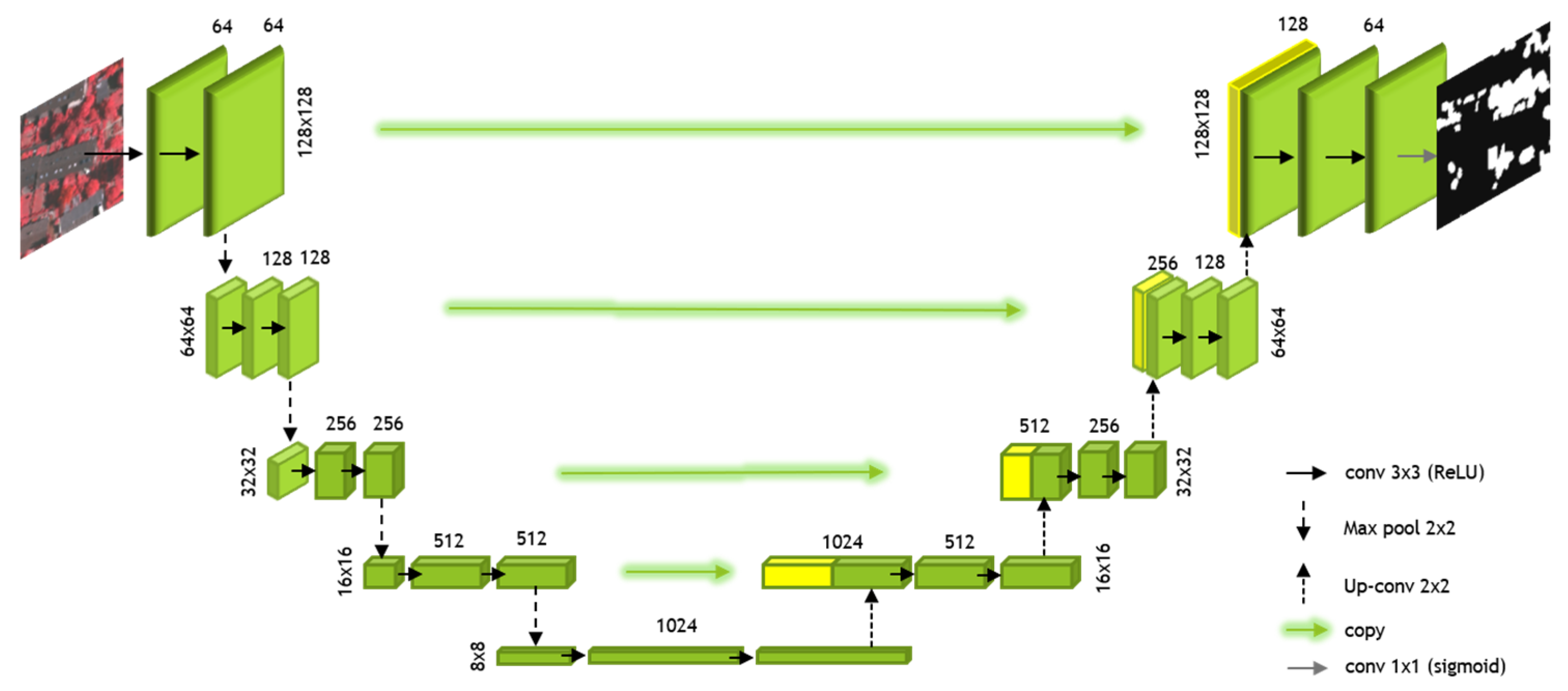
2.2. U-Net Architecture

The U-net architecture was designed for boundary detection and localization built from the FCN architecture [46]. It can be visualized as a symmetrical, U-shaped process with three main operations, convolution, max-pooling, and concatenation. Figure 2 gives a visual demonstration of the U-net architecture for tree canopy segmentation.
The U-net architecture consists of two paths, a contracting path as shown on the left side of the U-shape, and an expansive path as shown on the right side of the U-shape (Figure 2). In the contraction path, the black solid arrows refer to the convolution operation with a 3 × 3 kernel (conv 3 × 3). With the convolution, the number of channels increased from 3 to 64. The black dash arrows pointing down refer to the max-pooling operation with a 2 × 2 kernel (Max pool 2 × 2). In the max-pooling operation, the size of each feature map was reduced from 128 × 128 to 64 × 64. The preceding processes were repeated four times. At the bottom of the U-shape, an additional convolution operation was performed twice.
The expansive path restores the output image size from the contraction path to the original 128 × 128. The black dash arrows pointing up refer to the transposed convolution operation, which increases feature map size while decreasing channels. The green arrows pointing horizontally refer to a concatenation process that concatenates the output images from the previous step with the corresponding images from the contracting path. The concatenation process combines the information from the previous layers to achieve a more precise prediction. The preceding processes were repeated four times. The gray solid arrow at the upper right corner refers to a convolution operation with a 1 × 1 kernel (conv 1 × 1) to reshape the images according to prediction requirements.

2.3. Model Training

A total of four experiments were performed, with the spatial scales of input images being downsampled from 8 cm to 16 cm, 32 cm, 50 cm, and 100 cm, respectively. Figure 3 shows the model training workflow for the 16-cm experiment. The same workflow was repeated in the other three experiments. First, the original image with an 8 cm resolution was cropped into tiles of 256 × 256 pixels. Then, both the training and test datasets were downsampled to 16 cm, resulting in an image size of 128 × 128. Ninety percent of the tiles was used for training and 10% was used for testing. In the training process, 85% of the dataset was used for training and 15% was used for validation. We performed two evaluations to assess the model performance. In the first evaluation, the predicted output was first upsampled to 8 cm and then compared with the original 8-cm ground truth data. In the second evaluation, the ground truth data were resampled to the spatial resolution of the predicted output dataset before comparison. For example, to evaluate the performance of the 16-cm model, the ground truth data were downsampled to 16 cm before the accuracy assessment.

2.4. Dice Loss Function

In deep learning, neural networks are trained iteratively. At the end of each training, a loss function is used as a criterion to evaluate the prediction outcome. In this study, we employed the Dice loss function in the training process. The Dice loss function can be calculated from the Dice similarity coefficient (DSC), a statistic developed in the 1940s to gauge the similarity between two samples [49]. The Dice loss is given by
Dice loss = 1 2 i p i · g i i p i 2 + i g i 2
where p i and g i represent the pixel values of the i t h pixel in the training output and the corresponding ground truth images, respectively. In this study, the pixel values in the ground truth images are 0 and 1, referring to the non-tree class and tree class respectively. The Dice loss was calculated during the training process to provide an assessment of the training performance at each iterated epoch. The value of the Dice loss ranges from 0 to 1, where a lower value denotes a better training performance.
Figure 4 shows how the Dice loss changes at each epoch for the four experiments during the model training process. As the number of epochs increases, the Dice loss drops rapidly and stabilizes at Epoch 99, 243, 97, and 300 for the 16-cm, 32-cm, 50-cm, and 100-cm experiment, respectively.

2.5. Model Parameters and Environment

We used randomly selected tiles as our training datasets. For the experiment at each scale, 300 epochs with 8 batches per epoch were applied, and the learning rate was set at 0.0001 for all training models (Table 1). The Adam optimizer was utilized during the training process. We applied the horizontal shift augmentation to all images to increase the number of tiles in the training dataset. The number of shift pixels was different at each scale to ensure enough training samples were included in each model. The U-net architecture, as well as the whole semantic segmentation procedure, were implemented on the Tensorflow and Keras deep learning framework in Python programming language. All other processing and analyses were carried out using open-source modules, including GDAL, NumPy, Pandas, OpenCV, Scikit-learn, among others. The deep learning network experimentation and modeling were executed on the Google co-lab platform.

2.6. Performance Evaluation

We used four accuracy metrics to evaluate the performance of the U-net model, including the overall accuracy (OA), the DSC, the Intersection over Union (IoU) and the kappa coefficient (KC). All metrics were calculated based on a confusion matrix (Table 2), which records the percentage of pixels that are true positives (TP), false positives (FP), false negatives (FN), and true negatives (TN).
The OA was computed as the percentage of correctly classified pixels (Equation (2)). The DSC was a commonly used metric in semantic segmentation [50]. It was employed in Section 2.4 for calculating the loss function and was used here again for accuracy assessment (Equation (3)). The IoU, also known as the Jaccard Index, represents the ratio of the intersection to union between the predicted output and ground truth labeling images (Equation (4)) [51]. The KC, used widely in remote sensing applications, is a metric of how the classification results compare to values assigned by chance (Equation (5)) [52]. All metrics range from 0 to 1 with higher scores indicating higher accuracies.
OA = TP + TN TP + TN + FP + FN
DSC = 2 · TP 2 · TP + FP + FN
IoU = TP TP + FP + FN
KC = N × [ ( TN + FN ) · ( TN + FP ) + ( TP + FP ) · ( FN + TN ) ] N 2 [ ( TN + FN ) · ( TN + FP ) + ( TP + FP ) · ( FN + TN ) ] where   N   is   the   number   of   pixels

2.7. Object-Based Classification

The output of the U-net model was further compared to that of the object-based classification, a popular and widely applied approach to fine-scale land cover mapping. The object-based classification involves two main steps, segmentation and classification. We first used the multiresolution segmentation to group spectrally similar pixels into discrete objects. The shape, compactness, and scale factors were set to 0.1, 0.7, and 150, respectively. Based on a series of trial-and-error tests, an object with a mean value in the near-infrared band greater than 120 and a maximum difference value greater than 0.9 is being classified as tree canopy. The object-based classification was implemented in the eCognition software package [53].

3. Results

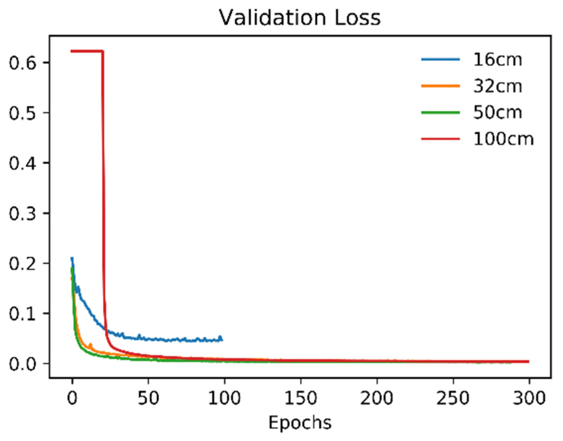
3.1. Performance of the U-Net Model at Multiple Scales

We performed two evaluations to assess the model performance. Evaluation 1 compared the predicted results with the 8-cm ground truth images. The accuracy metrics are shown in Table 3. All accuracy metric scores were higher than 0.91 except for those at the 100-cm scale. Consistently across all metrics, there was a score increase when the scale changed from 16 cm to 32 cm, followed by a slight decrease from 32 cm to 50 cm, and a drastic drop from 50 cm to 100 cm. The U-net model achieved the best performance on the 32-cm dataset and the worst on the 100-cm dataset. The highest metric score was 0.9914 (OA) and the lowest score was 0.7133 (IoU).
Evaluation 2 compared the predicted results with the ground truth images after adjusting to the spatial resolution of the predicted output. Table 4 shows the accuracy metric scores for Evaluation 2 at the four scales. First, all metric values were higher than those in Evaluation 1 regardless of scale. Second, all metrics were above 0.99 except for the 16-cm experiment. Similar to Evaluation 1, there was a substantial increase in all four metrics when the scale went from 16 cm to 32 cm. Different from Evaluation 1 though, the trend flattened out when the spatial resolution changed from 32 cm to 100 cm. Lastly, Evaluation 2 yielded much higher metric scores than Evaluation 1 at the 100-cm scale with the highest and lowest metric score of 0.9984 (OA) and 0.9934 (IoU), respectively.

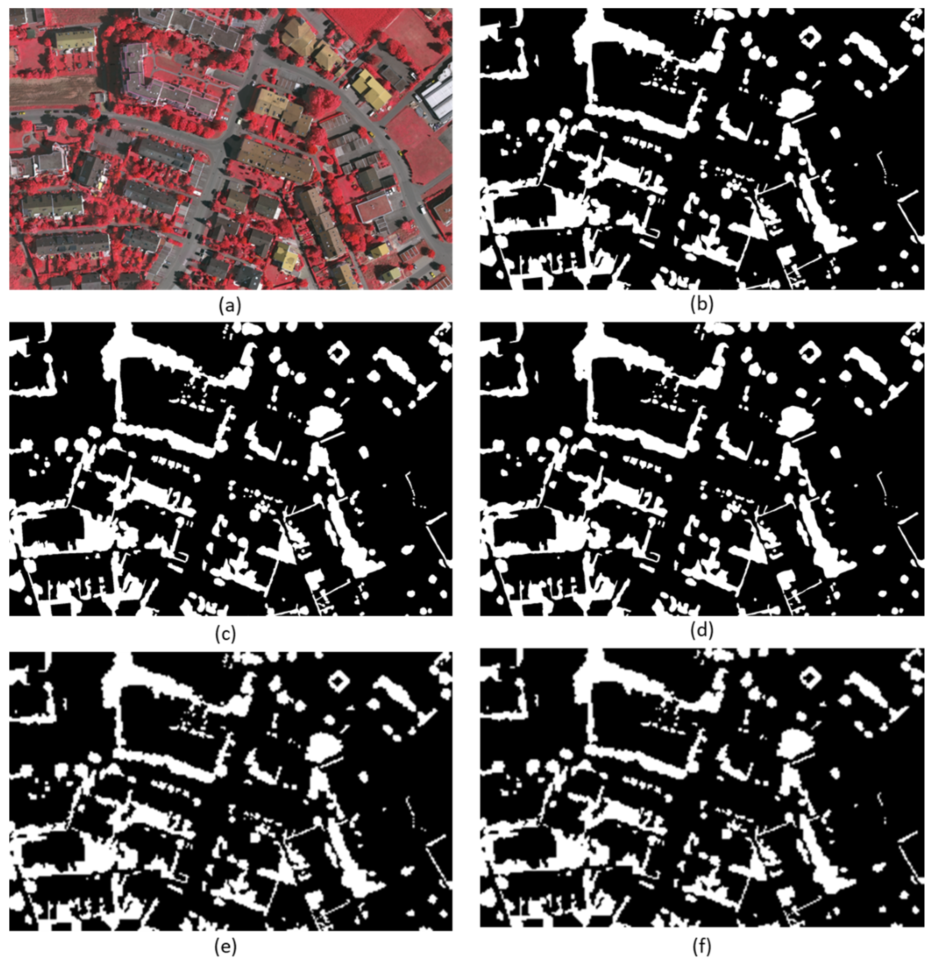
3.2. Visual Evaluation of the U-Net Performance

To visually assess the performance of the U-net model, we selected an example area with moderate tree canopy cover and compared the predicted output with the ground truth images. Figure 5 shows the selected area on an aerial photo (Figure 5a), ground truth images at 8 cm, 16 cm, and 100 cm (Figure 5b,d,f), and predicted output at 16 cm and 100 cm (Figure 5c,e). Overall, both U-net predictions (Figure 5c,e) showed great consistency with the ground truth images (Figure 5b,d,f). Specifically, the similar patterns in Figure 5b,c echoed the high accuracy scores at 16 cm in Evaluation 1 (Table 3). Because Figure 5d was downscaled to match the spatial resolution of Figure 5c, there was a higher level of similarity between Figure 5c,d than that between Figure 5c,b. This was corroborated by the higher accuracy scores in Table 4 than Table 3 at the 16-cm scale. A similar pattern was identified when comparing Figure 5e with Figure 5b,f. The lower metric values at the 100-cm scale in Table 3 were in part due to the blurry canopy boundaries as seen in Figure 5e as a result of down sampling. A better result was identified comparing Figure 5e with Figure 5f, consistent with the much higher accuracy scores at 100 cm in Table 3.

3.3. Performance Comparison between the U-Net and OBIA

Table 5 shows the accuracy scores of tree canopy mapping generated by the OBIA approach and the U-net model at the 16-cm scale. Both models were compared with the 8-cm ground truth data. For the OBIA, the highest metric score was 0.857 (OA) and the lowest was 0.489 (IoU). All the OBIA scores were lower than the U-net scores. It is worthy of note that even the highest score for the OBIA (OA: 0.857) was lower than the lowest score for the U-net (IoU: 0.9138), indicating that the U-net was superior to the OBIA in accurately mapping tree canopy at the 16-cm scale.
Figure 6 shows a comparison between the predicted output of the U-net and the OBIA in reference to the 8-cm ground truth image. By visual inspection, the U-net output (Figure 6c) showed a much better consistency with the ground truth image (Figure 6b) compared to the OBIA output (Figure 6d). There were much more misclassified pixels in the OBIA output than that in the U-net output, especially when identifying trees from grass and shrubs (yellow rectangle in Figure 6d). Further, the U-net model successfully distinguished trees from buildings, while both the OBIA and the ground truth failed to do so (red rectangle in Figure 6d). Overall, the U-net outperformed both the OBIA and the ground truth image in accurately extracting tree canopy cover from other complex urban land cover features.

4. Discussion

4.1. Performance of the U-Net in Urban Tree Canopy Mapping

In this study, we tested the effectiveness of the U-net in urban tree canopy mapping. We conducted the experiments at four different scales and performed two evaluations to assess the model performance from two different angles. Evaluation 1 (Table 3) compared the predicted output with the 8-cm ground truth. It aims to test the model performance operated on the datasets at different scales. Our results show that the U-net performed the best on the 32-cm dataset with an overall accuracy of 0.9914 (Table 3). While the 32-cm dataset is a coarser-resolution dataset compared to the 8-cm and 16-cm datasets, each image patch of the 32-cm dataset contains more geographic features than the other two. In deep learning, the spatial extent of the input is called “the receptive field”. It is defined as the size of the region in the input that produces the feature [54]. In this context, the receptive field indicates how many land cover features can be perceived from an input patch. Figure 7 shows examples of input image patches of three scales: (a) 16 cm, (b) 32 cm, and (c) 100 cm. According to Figure 7a, despite the higher spatial resolution, a 16-cm patch is too small to cover enough land cover objects such as buildings and trees with large crowns [54]. This in part explains the lower accuracies with the 8-cm and 16-cm datasets as they come with too small of a receptive field.
An overly large receptive field may also be problematic. Figure 7c shows an example of a 100-cm input patch. While it is large enough to include a significant number of land cover features, it comes with a cost of degradation of spatial details, resulting in a loss of locational accuracy especially at the tree edges. This is part of the reason why the DSC and KC values in the 100-cm experiment are much lower than the experiments performed at other scales. It is recognized that the size of the receptive field plays an important role in the training process of a deep learning neural network. Too small of a receptive field can limit the amount of contextual information while too large of a receptive field may cause a loss of spatial details and decline of locational accuracy [55]. An optimal receptive field ensures a good number of land cover features go to the training model while retaining the spatial accuracy of the dataset. That is the case for the 32-cm dataset in our study, which achieves the highest accuracy scores and the best model performance (Table 3). It is worthy of note that even with the 100-cm dataset, the U-net is still able to achieve an OA of 0.9324 (Table 3), indicating the overall effectiveness of the U-net architecture in urban tree canopy mapping.
We performed Evaluation 2 to assess the accuracy of the U-net models based on input and output of the same spatial resolution. This evaluation is essential because high-resolution ground truth data are not always attainable. Results show that the performance of the U-net architecture is exceptional based on the incredibly high accuracy metric scores (Table 4). All metric scores are above 0.99 for scales from 32 cm to 100 cm. These results indicate promising applications of the U-net architecture. An example is the National Agriculture Imagery Program (NAIP), which offers freely accessible satellite imagery across the United States at 1-m (100-cm) spatial resolution. From the results in Table 4, all metric scores are above 0.99 at the 100-cm scale, suggesting a highly effective and promising application of the U-net model to fine-scale land cover mapping based on NAIP data.

4.2. Comparison between the U-Net and OBIA

The OBIA has been a mainstream approach for high-resolution land cover mapping during the last decade. Myint et al. (2011) used the OBIA method to extract major land cover types in Phoenix from QuickBird images. In their study, the DSC score for the tree class was 0.8551 [28]. Over the same study area, Li et al. (2014) developed another set of decision rules using the NAIP imagery and successfully raised the DSC score to 0.88 [32]. Apart from the multispectral satellite imagery, Zhou (2013) supplemented the height and intensity from the LiDAR data and yielded a DSC score of 0.939 [56]. With a large number of existing studies using the OBIA approach, our study using the U-net model achieves a higher mapping accuracy than almost all the OBIA-based studies in the literature (DSC: 0.9816).
To further compare the performance of the U-net with the OBIA, we selected a sample study area with a variety of land cover types and applied the 16-cm U-net model and the OBIA approach to the same area. Figure 6 provides a visual comparison between the OBIA and U-net output. Urban tree canopy mapping is challenging because trees are typically planted on grassland or closely adjacent to buildings (Figure 6a). The U-net model has the unique capacity of accurately distinguishing trees from grass and buildings (Figure 6c) while the OBIA approach is not as effective (Figure 6d).
One of the major downsides of the OBIA is a requisite for enough expert knowledge of the study area and the land cover types under investigation [57]. In contrast, the U-net automatically learns the features in the study area without too much human intervention on parameter decisions [58]. Moreover, the U-net, as a deep learning network, comes with a very high level of automation with a minimal need of manual editing after the classification. This is a prominent advantage of the U-net over the OBIA because the accuracy of the OBIA depends to a great extent on post-classification manual editing which is time-consuming and labor-intensive. As the U-net is free of manual editing, it has a great potential to become a mainstream mapping tool especially when dealing with large amounts of high-resolution data.

4.3. Comparison between the U-Net and Other Deep Learning Methods

The test dataset of this study was made available from the ISPRS 2D Semantic Labeling Contest. The dataset contains orthophotos, digital surface model (DSM) images, and normalized DSM (nDSM) images over the Vaihingen city in Germany. The same set of data was utilized by a number of deep learning studies on tree canopy mapping. Table 6 lists a couple of these studies along with their methods, datasets, and DSC values on the tree class. Audebert et al. (2016) utilized the multimodal and multi-scale deep networks on the orthophotos. The DSC score on the tree class was 0.899 [59]. Sang and Minh (2018) used both the orthophotos and the nDSM images to train a fully convolutional neural network (FCNN). The classification accuracy was not improved in spite of adding the nDSM images on top of the orthophotos [60]. Paisitriangkrai et al. (2015) took advantage of the entire dataset (all three data sets) to train a multi-resolution convolutional neural network, yielding a DSC value of 0.8497. Compared to the above studies using the Vaihingen dataset, our U-net model conducted at 16 cm, 32 cm, and 50 cm outperforms all of them with a DSC of above 0.95. Note that adding DSM images fails to improve the overall model performance. Our best-performing model, the 32-cm U-net model, achieves a DSC of 0.9816. This surpasses the DSC of the contest winner (0.908), indicating the exceptional effectiveness of the U-net architecture on tree canopy mapping.
Numerous studies have made modifications to the U-net architecture in an attempt to improve the model performance [42,62,63]. For instance, Diakogiannis et al. (2020) integrated the U-net with the residual neural network using high-resolution orthophotos and DSM images [64]. The dataset they used was also published by the ISPRS 2D Semantic Labeling Contest [65] and was similar to the Vaihingen dataset used in this study. The modified framework achieved a DSC score of 0.8917 on the tree class compared to 0.9816 in this study (Table 3). While the U-net is simpler, it is more effective than the other, more complex, deep learning architecture. This is consistent with Ba and Caruana (2014) that while depth can make the learning process easier, it may not always be essential [66]. Choosing the most efficient and suitable neural network is a top priority to ensure the best overall performance of a deep learning framework.

5. Conclusions

Mapping urban trees using high-resolution remote sensing imagery is important for understanding urban forest structure for better forest management. In this study, we applied the U-net to urban tree canopy mapping using high-resolution aerial photos. We tested the effectiveness of the U-net at four different scales and performed two evaluations to assess the model performance from two different angles. Evaluation 1 shows that the U-net performed the best on the 32-cm dataset, with an overall accuracy of 0.9914. The experiments conducted at four scales indicate the significance of an optimal receptive field for training a deep learning model. Evaluation 2 shows that the U-net can be used as a highly effective and promising tool for fine-scale land cover mapping with exceptional accuracy scores. Moreover, the comparison experiment shows the outstanding performance of the U-net compared to the widely used OBIA approach and other deep learning methods.
This study shows the utility of the U-net in urban tree canopy mapping and discusses the possibility of extending its use to other applications. A broad application of the U-net to high-resolution land cover mapping faces several challenges. First, as with any fine-scale land cover mapping tasks, the availability of freely accessible high-resolution imagery is an issue. U-net model training often requires satellite images with a spatial resolution of 1 m or finer. It remains a challenge to acquire very high-resolution data for regions of interest at desired times. Second, the lack of publicly available training datasets poses another problem. Ground truth data are usually produced by local government or research institutions through field surveys or manual digitization. The process of generating accurate ground truth data is a complex and laborious task. A possible solution is to introduce the techniques and strategies in transfer learning. Approaches such as pre-training, fine-tuning, and domain adaptation can alleviate the dependence on large labeled dataset. Therefore, integrating the U-net and transfer learning is a potential direction of future research.

Author Contributions

Conceptualization, Z.W.; methodology, Z.W. and M.X.; data curation, Z.W.; original draft preparation, Z.W. and C.F.; review and editing, C.F. and M.X.; visualization, Z.W.; supervision, C.F. All authors have read and agreed to the published version of the manuscript.

Funding

This research was funded by the National Science Foundation, grant number 2019609.

Data Availability Statement

Publicly available datasets used in this study can be accessed from https://www2.isprs.org/commissions/comm2/wg4/benchmark/2d-sem-label-vaihingen/ (accessed on 3 April 2021).

Conflicts of Interest

The authors declare no conflict of interest.

References

  1. Buyantuyev, A.; Wu, J. Urban Heat Islands and Landscape Heterogeneity: Linking Spatiotemporal Variations in Surface Temperatures to Land-Cover and Socioeconomic Patterns. Landsc. Ecol. 2010, 25, 17–33. [Google Scholar] [CrossRef]
  2. Dwyer, M.C.; Miller, R.W. Using GIS to Assess Urban Tree Canopy Benefits and Surrounding Greenspace Distributions. J. Arboric. 1999, 25, 102–107. [Google Scholar]
  3. Loughner, C.P.; Allen, D.J.; Zhang, D.-L.; Pickering, K.E.; Dickerson, R.R.; Landry, L. Roles of Urban Tree Canopy and Buildings in Urban Heat Island Effects: Parameterization and Preliminary Results. J. Appl. Meteorol. Climatol. 2012, 51, 1775–1793. [Google Scholar] [CrossRef]
  4. Nowak, D.J.; Crane, D.E. Carbon Storage and Sequestration by Urban Trees in the USA. Environ. Pollut. 2002, 116, 381–389. [Google Scholar] [CrossRef]
  5. Pandit, R.; Polyakov, M.; Sadler, R. Valuing Public and Private Urban Tree Canopy Cover. Aust. J. Agric. Resour. Econ. 2014, 58, 453–470. [Google Scholar] [CrossRef] [Green Version]
  6. Payton, S.; Lindsey, G.; Wilson, J.; Ottensmann, J.R.; Man, J. Valuing the Benefits of the Urban Forest: A Spatial Hedonic Approach. J. Environ. Plan. Manag. 2008, 51, 717–736. [Google Scholar] [CrossRef]
  7. Ulmer, J.M.; Wolf, K.L.; Backman, D.R.; Tretheway, R.L.; Blain, C.J.; O’Neil-Dunne, J.P.; Frank, L.D. Multiple Health Benefits of Urban Tree Canopy: The Mounting Evidence for a Green Prescription. Health Place 2016, 42, 54–62. [Google Scholar] [CrossRef]
  8. Cities and Communities in the US Losing 36 Million Trees a Year. Available online: https://www.sciencedaily.com/releases/2018/04/180418141323.htm (accessed on 19 October 2020).
  9. Grove, J.M.; O’Neil-Dunne, J.; Pelletier, K.; Nowak, D.; Walton, J. A Report on New York City’s Present and Possible Urban Tree Canopy; United States Department of Agriculture, Forest Service: South Burlington, VT, USA, 2006.
  10. Fuller, R.A.; Gaston, K.J. The Scaling of Green Space Coverage in European Cities. Biol. Lett. 2009, 5, 352–355. [Google Scholar] [CrossRef] [Green Version]
  11. King, K.L.; Locke, D.H. A Comparison of Three Methods for Measuring Local Urban Tree Canopy Cover. Available online: https://www.nrs.fs.fed.us/pubs/42933 (accessed on 14 June 2020).
  12. Tree Cover %—How Does Your City Measure Up? | DeepRoot Blog. Available online: https://www.deeproot.com/blog/blog-entries/tree-cover-how-does-your-city-measure-up (accessed on 14 June 2020).
  13. Fan, C.; Johnston, M.; Darling, L.; Scott, L.; Liao, F.H. Land Use and Socio-Economic Determinants of Urban Forest Structure and Diversity. Landsc. Urban Plan. 2019, 181, 10–21. [Google Scholar] [CrossRef]
  14. Li, M.; Zang, S.; Zhang, B.; Li, S.; Wu, C. A Review of Remote Sensing Image Classification Techniques: The Role of Spatio-Contextual Information. Eur. J. Remote Sens. 2014, 47, 389–411. [Google Scholar] [CrossRef]
  15. LP DAAC—MODIS Overview. Available online: https://lpdaac.usgs.gov/data/get-started-data/collection-overview/missions/modis-overview/#modis-metadata (accessed on 14 December 2020).
  16. The Thematic Mapper. Landsat Science. Available online: https://landsat.gsfc.nasa.gov/the-thematic-mapper/ (accessed on 14 June 2020).
  17. SPOT—CNES. Available online: https://web.archive.org/web/20131006213713/http://www.cnes.fr/web/CNES-en/1415-spot.php (accessed on 14 June 2020).
  18. Baeza, S.; Paruelo, J.M. Land Use/Land Cover Change (2000–2014) in the Rio de La Plata Grasslands: An Analysis Based on MODIS NDVI Time Series. Remote Sens. 2020, 12, 381. [Google Scholar] [CrossRef] [Green Version]
  19. Ferri, S.; Syrris, V.; Florczyk, A.; Scavazzon, M.; Halkia, M.; Pesaresi, M. A New Map of the European Settlements by Automatic Classification of 2.5 m Resolution SPOT Data. In Proceedings of the 2014 IEEE Geoscience and Remote Sensing Symposium, Quebec City, QC, Canada, 13–18 July 2014; pp. 1160–1163. [Google Scholar]
  20. Tran, D.X.; Pla, F.; Latorre-Carmona, P.; Myint, S.W.; Caetano, M.; Kieu, H.V. Characterizing the Relationship between Land Use Land Cover Change and Land Surface Temperature. ISPRS J. Photogramm. Remote Sens. 2017, 124, 119–132. [Google Scholar] [CrossRef] [Green Version]
  21. Alonzo, M.; McFadden, J.P.; Nowak, D.J.; Roberts, D.A. Mapping Urban Forest Structure and Function Using Hyperspectral Imagery and Lidar Data. Urban For. Urban Green. 2016, 17, 135–147. [Google Scholar] [CrossRef] [Green Version]
  22. Alonzo, M.; Bookhagen, B.; Roberts, D.A. Urban Tree Species Mapping Using Hyperspectral and Lidar Data Fusion. Remote Sens. Environ. 2014, 148, 70–83. [Google Scholar] [CrossRef]
  23. MacFaden, S.W.; O’Neil-Dunne, J.P.; Royar, A.R.; Lu, J.W.; Rundle, A.G. High-Resolution Tree Canopy Mapping for New York City Using LIDAR and Object-Based Image Analysis. J. Appl. Remote Sens. 2012, 6, 063567. [Google Scholar] [CrossRef]
  24. Ronda, R.J.; Steeneveld, G.J.; Heusinkveld, B.G.; Attema, J.J.; Holtslag, A.A.M. Urban Finescale Forecasting Reveals Weather Conditions with Unprecedented Detail. Bull. Am. Meteorol. Soc. 2017, 98, 2675–2688. [Google Scholar] [CrossRef]
  25. Yang, C.-C.; Prasher, S.O.; Enright, P.; Madramootoo, C.; Burgess, M.; Goel, P.K.; Callum, I. Application of Decision Tree Technology for Image Classification Using Remote Sensing Data. Agric. Syst. 2003, 76, 1101–1117. [Google Scholar] [CrossRef]
  26. Zhu, G.; Blumberg, D.G. Classification Using ASTER Data and SVM Algorithms;: The Case Study of Beer Sheva, Israel. Remote Sens. Environ. 2002, 80, 233–240. [Google Scholar] [CrossRef]
  27. Ahmed, K.R.; Akter, S. Analysis of Landcover Change in Southwest Bengal Delta Due to Floods by NDVI, NDWI and K-Means Cluster with Landsat Multi-Spectral Surface Reflectance Satellite Data. Remote Sens. Appl. Soc. Environ. 2017, 8, 168–181. [Google Scholar] [CrossRef]
  28. Myint, S.W.; Gober, P.; Brazel, A.; Grossman-Clarke, S.; Weng, Q. Per-Pixel vs. Object-Based Classification of Urban Land Cover Extraction Using High Spatial Resolution Imagery. Remote Sens. Environ. 2011, 115, 1145–1161. [Google Scholar] [CrossRef]
  29. Wang, P.; Feng, X.; Zhao, S.; Xiao, P.; Xu, C. Comparison of Object-Oriented with Pixel-Based Classification Techniques on Urban Classification Using TM and IKONOS Imagery; Ju, W., Zhao, S., Eds.; International Society for Optics and Photonics: Nanjing, China, 2007; p. 67522J. [Google Scholar]
  30. De Luca, G.; Silva, J.M.N.; Cerasoli, S.; Araújo, J.; Campos, J.; Di Fazio, S.; Modica, G. Object-Based Land Cover Classification of Cork Oak Woodlands Using UAV Imagery and Orfeo ToolBox. Remote Sens. 2019, 11, 1238. [Google Scholar] [CrossRef] [Green Version]
  31. Hossain, M.D.; Chen, D. Segmentation for Object-Based Image Analysis (Obia): A Review of Algorithms and Challenges from Remote Sensing Perspective. ISPRS J. Photogramm. Remote Sens. 2019, 150, 115–134. [Google Scholar] [CrossRef]
  32. Li, X.; Myint, S.W.; Zhang, Y.; Galletti, C.; Zhang, X.; Turner, B.L., II. Object-Based Land-Cover Classification for Metropolitan Phoenix, Arizona, Using Aerial Photography. Int. J. Appl. Earth Obs. Geoinf. 2014, 33, 321–330. [Google Scholar] [CrossRef]
  33. Pashaei, M.; Kamangir, H.; Starek, M.J.; Tissot, P. Review and Evaluation of Deep Learning Architectures for Efficient Land Cover Mapping with UAS Hyper-Spatial Imagery: A Case Study Over a Wetland. Remote Sens. 2020, 12, 959. [Google Scholar] [CrossRef] [Green Version]
  34. Zhu, X.X.; Tuia, D.; Mou, L.; Xia, G.-S.; Zhang, L.; Xu, F.; Fraundorfer, F. Deep Learning in Remote Sensing: A Comprehensive Review and List of Resources. IEEE Geosci. Remote Sens. Mag. 2017, 5, 8–36. [Google Scholar] [CrossRef] [Green Version]
  35. Ondruska, P.; Dequaire, J.; Wang, D.Z.; Posner, I. End-to-End Tracking and Semantic Segmentation Using Recurrent Neural Networks. arXiv 2016, arXiv:1604.05091. [Google Scholar]
  36. Qian, R.; Zhang, B.; Yue, Y.; Wang, Z.; Coenen, F. Robust Chinese Traffic Sign Detection and Recognition with Deep Convolutional Neural Network. In Proceedings of the 2015 11th International Conference on Natural Computation (ICNC), Zhangjiajie, China, 15–17 August 2015; pp. 791–796. [Google Scholar] [CrossRef]
  37. Yuan, Q.; Shen, H.; Li, T.; Li, Z.; Li, S.; Jiang, Y.; Xu, H.; Tan, W.; Yang, Q.; Wang, J. Deep Learning in Environmental Remote Sensing: Achievements and Challenges. Remote Sens. Environ. 2020, 241, 111716. [Google Scholar] [CrossRef]
  38. Krizhevsky, A.; Sutskever, I.; Hinton, G.E. Imagenet Classification with Deep Convolutional Neural Networks. In Proceedings of the Advances in neural information processing systems, Lake Tahoe, CA, USA, 3–6 December 2012; pp. 1097–1105. [Google Scholar]
  39. Long, J.; Shelhamer, E.; Darrell, T. Fully Convolutional Networks for Semantic Segmentation. In Proceedings of the IEEE Conference on Computer Vision and Pattern Recognition, Boston, MA, USA, 7–12 June 2015; pp. 3431–3440. [Google Scholar]
  40. Pan, Z.; Xu, J.; Guo, Y.; Hu, Y.; Wang, G. Deep Learning Segmentation and Classification for Urban Village Using a Worldview Satellite Image Based on U-Net. Remote Sens. 2020, 12, 1574. [Google Scholar] [CrossRef]
  41. Falk, T.; Mai, D.; Bensch, R.; Çiçek, Ö.; Abdulkadir, A.; Marrakchi, Y.; Böhm, A.; Deubner, J.; Jäckel, Z.; Seiwald, K. U-Net: Deep Learning for Cell Counting, Detection, and Morphometry. Nat. Methods 2019, 16, 67–70. [Google Scholar] [CrossRef]
  42. Çiçek, Ö.; Abdulkadir, A.; Lienkamp, S.S.; Brox, T.; Ronneberger, O. 3D U-Net: Learning Dense Volumetric Segmentation from Sparse Annotation. In Proceedings of the International Conference on Medical Image Computing and Computer-Assisted Intervention, Athens, Greece, 17–21 October 2016; Springer: Berlin/Heidelberg, Germany, 2016; pp. 424–432. [Google Scholar]
  43. Esser, P.; Sutter, E.; Ommer, B. A Variational U-Net for Conditional Appearance and Shape Generation. In Proceedings of the IEEE Conference on Computer Vision and Pattern Recognition, Salt Lake City, UT, USA, 18–22 June 2018; pp. 8857–8866. [Google Scholar]
  44. Macartney, C.; Weyde, T. Improved Speech Enhancement with the Wave-u-Net. arXiv 2018, arXiv:1811.11307. [Google Scholar]
  45. Feng, W.; Sui, H.; Huang, W.; Xu, C.; An, K. Water Body Extraction from Very High-Resolution Remote Sensing Imagery Using Deep U-Net and a Superpixel-Based Conditional Random Field Model. IEEE Geosci. Remote Sens. Lett. 2018, 16, 618–622. [Google Scholar] [CrossRef]
  46. Ronneberger, O.; Fischer, P.; Brox, T. U-Net: Convolutional Networks for Biomedical Image Segmentation. In Proceedings of the Medical Image Computing and Computer-Assisted Intervention—MICCAI 2015; Navab, N., Hornegger, J., Wells, W.M., Frangi, A.F., Eds.; Springer International Publishing: Cham, Switzerland, 2015; pp. 234–241. [Google Scholar]
  47. Wagner, F.H.; Dalagnol, R.; Tarabalka, Y.; Segantine, T.Y.; Thomé, R.; Hirye, M. U-Net-Id, an Instance Segmentation Model for Building Extraction from Satellite Images—Case Study in the Joanópolis City, Brazil. Remote Sens. 2020, 12, 1544. [Google Scholar] [CrossRef]
  48. Freudenberg, M.; Nölke, N.; Agostini, A.; Urban, K.; Wörgötter, F.; Kleinn, C. Large Scale Palm Tree Detection In High Resolution Satellite Images Using U-Net. Remote Sens. 2019, 11, 312. [Google Scholar] [CrossRef] [Green Version]
  49. Dice, L.R. Measures of the Amount of Ecologic Association between Species. Ecology 1945, 26, 297–302. [Google Scholar] [CrossRef]
  50. Bertels, J.; Eelbode, T.; Berman, M.; Vandermeulen, D.; Maes, F.; Bisschops, R.; Blaschko, M.B. Optimizing the Dice Score and Jaccard Index for Medical Image Segmentation: Theory and Practice. In Proceedings of the International Conference on Medical Image Computing and Computer-Assisted Intervention, Shenzhen, China, 13–17 October 2019; Springer: Berlin/Heidelberg, Germany, 2019; pp. 92–100. [Google Scholar]
  51. Hamers, L. Similarity Measures in Scientometric Research: The Jaccard Index versus Salton’s Cosine Formula. Inf. Process. Manag. 1989, 25, 315–318. [Google Scholar] [CrossRef]
  52. Stehman, S. Estimating the Kappa Coefficient and Its Variance under Stratified Random Sampling. Photogramm. Eng. Remote Sens. 1996, 62, 401–407. [Google Scholar]
  53. ECognition. Trimble Geospatial. Available online: https://geospatial.trimble.com/products-and-solutions/ecognition (accessed on 10 September 2020).
  54. Araujo, A.; Norris, W.; Sim, J. Computing Receptive Fields of Convolutional Neural Networks. Distill 2019, 4, e21. [Google Scholar] [CrossRef]
  55. Qin, X.; Wu, C.; Chang, H.; Lu, H.; Zhang, X. Match Feature U-Net: Dynamic Receptive Field Networks for Biomedical Image Segmentation. Symmetry 2020, 12, 1230. [Google Scholar] [CrossRef]
  56. Zhou, W. An Object-Based Approach for Urban Land Cover Classification: Integrating LiDAR Height and Intensity Data. IEEE Geosci. Remote Sens. Lett. 2013, 10, 928–931. [Google Scholar] [CrossRef]
  57. Whiteside, T.G.; Boggs, G.S.; Maier, S.W. Comparing Object-Based and Pixel-Based Classifications for Mapping Savannas. Int. J. Appl. Earth Obs. Geoinf. 2011, 13, 884–893. [Google Scholar] [CrossRef]
  58. Liang, H.; Li, Q. Hyperspectral Imagery Classification Using Sparse Representations of Convolutional Neural Network Features. Remote Sens. 2016, 8, 99. [Google Scholar] [CrossRef] [Green Version]
  59. Audebert, N.; Le Saux, B.; Lefèvre, S. Semantic Segmentation of Earth Observation Data Using Multimodal and Multi-Scale Deep Networks. In Proceedings of the Asian Conference on Computer Vision, Taipei, Taiwan, 20–24 November 2016; Springer: Berlin/Heidelberg, Germany, 2016; pp. 180–196. [Google Scholar]
  60. Sang, D.V.; Minh, N.D. Fully Residual Convolutional Neural Networks for Aerial Image Segmentation. In Proceedings of the Ninth International Symposium on Information and Communication Technology, Da Nang City, Viet Nam, 6–7 December 2018; pp. 289–296. [Google Scholar]
  61. Paisitkriangkrai, S.; Sherrah, J.; Janney, P.; Van-Den Hengel, A. Effective Semantic Pixel Labelling with Convolutional Networks and Conditional Random Fields. In Proceedings of the 2015 IEEE Conference on Computer Vision and Pattern Recognition Workshops (CVPRW), Boston, MA, USA, 7–12 June 2015; pp. 36–43. [Google Scholar]
  62. Zhang, J.; Du, J.; Liu, H.; Hou, X.; Zhao, Y.; Ding, M. LU-NET: An Improved U-Net for Ventricular Segmentation. IEEE Access 2019, 7, 92539–92546. [Google Scholar] [CrossRef]
  63. Zhang, Z.; Liu, Q.; Wang, Y. Road Extraction by Deep Residual U-Net. IEEE Geosci. Remote Sens. Lett. 2018, 15, 749–753. [Google Scholar] [CrossRef] [Green Version]
  64. Diakogiannis, F.I.; Waldner, F.; Caccetta, P.; Wu, C. Resunet-a: A Deep Learning Framework for Semantic Segmentation of Remotely Sensed Data. ISPRS J. Photogramm. Remote Sens. 2020, 162, 94–114. [Google Scholar] [CrossRef] [Green Version]
  65. 2D Semantic Labeling—Potsdam. Available online: https://www2.isprs.org/commissions/comm2/wg4/benchmark/2d-sem-label-potsdam/ (accessed on 18 January 2021).
  66. Ba, J.; Caruana, R. Do Deep Nets Really Need to Be Deep? Adv. Neural Inf. Process. Syst. 2014, 27, 2654–2662. [Google Scholar]
Figure 1. Study area located in Vaihingen, Germany.
Remotesensing 13 01749 g001
Figure 2. The U-net architecture for tree canopy segmentation.
Remotesensing 13 01749 g002
Figure 3. Flowchart of the U-net model for the 16-cm experiment.
Remotesensing 13 01749 g003
Figure 4. Dice loss for the four models in the training process.
Remotesensing 13 01749 g004
Figure 5. An example area of the tree canopy output map from the U-net: (a) original orthophoto, (b) 8-cm ground truth image, (c) 16-cm predicted tree canopy, (d) 16-cm ground truth image, (e) 100-cm predicted tree canopy, and (f) 100-cm ground truth image (white areas refer to tree canopy pixels; black areas refer to non-tree pixels).
Remotesensing 13 01749 g005
Figure 6. Comparison of the urban tree canopy segmentation between the U-net and OBIA: (a) original orthophoto, (b) ground truth image, (c) predicted output of the U-net, and (d) OBIA classification result (white areas refer to tree canopy pixels; black areas refer to non-tree pixels; red rectangle shows an example area where trees are adjacent to buildings; yellow rectangle shows an example area where there is a mix of trees, grass, and shrubs).
Remotesensing 13 01749 g006
Figure 7. Examples of the input image patch for the U-net: (a) 16-cm input image patch, (b) 32-cm input image patch, (c) 100-cm input image patch.
Remotesensing 13 01749 g007
Table 1. Model parameters for the four experiments.
Number of EpochsNumber of BatchesFinish EpochLearning RateNumber of Tiles
16 cm3008910.000112,627
32 cm3008420.000114,887
50 cm30082380.00016428
100 cm30081330.00014683
Table 2. Confusion matrix for accuracy assessment.
Ground Truth/
Prediction
TreeNon-Tree
TreeTP aFP b
Non-treeFN cTN d
a TP: true positive. b FP: false positive. c FN: false negative. d TN: true negative.
Table 3. Accuracy metric scores at the four scales in Evaluation 1.
ScaleOADSCIoUKC
16 cm0.97910.95500.91380.9411
32 cm0.99140.98160.96380.9770
50 cm0.98810.97410.94960.9664
100 cm0.93240.83270.71330.7917
Table 4. Accuracy metric scores at the four scales in Evaluation 2.
ScaleOADSCIoUKC
16 cm0.97980.95680.91710.9436
32 cm0.99820.99620.99250.9952
50 cm0.99870.99720.99440.9963
100 cm0.99840.99670.99340.9983
Table 5. Comparison of tree canopy mapping accuracy between OBIA and U-net (16 cm).
IoUDSCOAKC
OBIA0.4890.6570.8570.5681
U-net (16 cm)0.91380.95500.97910.9411
Table 6. Performance comparison of the U-net with other deep learning methods on the same dataset.
MethodDatasetDSC
Multimodal and Multi-scale Deep Networks [59]Orthophoto0.899
Fully Convolutional Neural Network (FCNN) [60]Orthophoto + nDSM0.899
Multi-resolution Convolutional Neural Network [61]Orthophoto + nDSM + DSM0.8497
32-cm U-net (this study)Orthophoto0.9816
Publisher’s Note: MDPI stays neutral with regard to jurisdictional claims in published maps and institutional affiliations.

