Acoustic Seafloor Classification Using the Weyl Transform of Multibeam Echosounder Backscatter Mosaic ^†

Abstract

The use of multibeam echosounder systems (MBES) for detailed seafloor mapping is increasing at a fast pace. Due to their design, enabling continuous high-density measurements and the coregistration of seafloor’s depth and reflectivity, MBES has become a fundamental instrument in the advancing field of acoustic seafloor classification (ASC). With these data becoming available, recent seafloor mapping research focuses on the interpretation of the hydroacoustic data and automated predictive modeling of seafloor composition. While a methodological consensus on which seafloor sediment classification algorithm and routine does not exist in the scientific community, it is expected that progress will occur through the refinement of each stage of the ASC pipeline: ranging from the data acquisition to the modeling phase. This research focuses on the stage of the feature extraction; the stage wherein the spatial variables used for the classification are, in this case, derived from the MBES backscatter data. This contribution explored the sediment classification potential of a textural feature based on the recently introduced Weyl transform of 300 kHz MBES backscatter imagery acquired over a nearshore study site in Belgian Waters. The goodness of the Weyl transform textural feature for seafloor sediment classification was assessed in terms of cluster separation of Folk’s sedimentological categories (4-class scheme). Class separation potential was quantified at multiple spatial scales by cluster silhouette coefficients. Weyl features derived from MBES backscatter data were found to exhibit superior thematic class separation compared to other well-established textural features, namely: (1) First-order Statistics, (2) Gray Level Co-occurrence Matrices (GLCM), (3) Wavelet Transform and (4) Local Binary Pattern (LBP). Finally, by employing a Random Forest (RF) categorical classifier, the value of the proposed textural feature for seafloor sediment mapping was confirmed in terms of global and by-class classification accuracies, highest for models based on the backscatter Weyl features. Further tests on different backscatter datasets and sediment classification schemes are required to further elucidate the use of the Weyl transform of MBES backscatter imagery in the context of seafloor mapping.

1. Introduction

Human pressures on the marine environment are rapidly increasing due to a multitude of concurrently developing economic sectors and interests [1]. At a European level, human activities in the marine environment are regulated by maritime spatial plans (MSP) implemented by each member state under the EU Maritime Spatial Planning Directive 2014/89/EU. The goal of the MSP is to accommodate the designation of space suitable for human activities, while also ensuring environmental protection via the exclusion and/or regulation of activities within, for example, Habitat Directive (HD) and/or Marine Protected Areas (MPAs) [2,3]. The detailed understanding of the type and extent of seafloor sediments, recognized as a keystone surrogate for marine life [4,5], underpins the effective implementation of an ecosystem-based management, including setting the baselines for environmental monitoring. The production of detailed seafloor sediment maps (referred to as benthic habitat maps, when including a biological component, and/or substrate maps, when reporting only abiotic information of the sediment), has drastically matured over the past decades, owing to significant technological developments of the remote sensing instrumentation such as multibeam echosounder systems (MBES) [6,7], as well as to drastic improvements in hydroacoustic data processing [8,9]. This has allowed marine scientists to access seafloor imagery approaching the level of detail encountered in the terrestrial remote sensing realm. As a result, this has enabled the development of equivalent “land cover classification” approaches for the underwater environment [3,10,11,12].

Due to their design, enabling full-coverage and high-density measurements and recording both seafloor bathymetry and backscatter strength, MBES have become a central hydroacoustic remote sensing technology, routinely employed since the late 1980s for standard mapping operations (e.g., hydrographic surveying) [13]. Seafloor bathymetry (depth) and reflectivity (backscatter strength) are the primary data recorded by a MBES. Bathymetry, measured from echoes flight times and angles, is processed to provide continuous topographic information. Backscatter, retained until recently only as a sonar byproduct, is now recognized as a proxy of the seafloor nature (texture and composition), related to five fundamental physical quantities: (a) the acoustic impedance contrast (or hardness), (b) the seafloor roughness, (c) the water-sediment interface volume heterogeneity, (d) the acoustical frequency and (e) the sound pulse angle of incidence onto the seafloor [8]. Due to the scattering properties of different seafloor substrates and features, backscatter can help determine bottom type [14,15,16]. Put simply, using MBES backscatter for sediment characterization can be interpreted as the identification of “the characteristics and spatial organization of seafloor patches and/or signatures with common acoustic responses and the measurable characteristics of this response” [17].

The backscatter strength returning to the sonar receiver is dependent on geological conditions, sonar equipment, environmental factors, etc. Moreover, various third-party processing software always cannot provide enough details of the compensation algorithm applied in their products, which hinders the subsequent data processing work. To exploit backscatter data for image analysis, rigorous processing steps must be taken to radiometrically and geometrically reduce the data and different backscatter datatypes can be obtained [8,9,17]. Both signal and image-based backscatter can be used for seafloor sediment characterization. Signal-based methods exploit the inherent property of the backscatter angular dependence (i.e., the physical variation in backscatter intensity with angle of incidence onto the seafloor) and refer to Angular Range Analysis (ARA), identifying the characteristics of the angular backscatter response curve describing sediment type [18]. Image-based methods rely on the backscatter imagery (backscatter mosaic); removing the angular dependence via statistical compensation and normalized and referenced to a conventional incidence angle (or a limited range of angles), in such a way that the whole seafloor scene seems to be observed from one same incidence angle [8]. The backscatter imagery is gridded as a function of the bathymetric resolution and presented in a georeferenced frame, generally in the form of a grey-scale image displaying the continuum of geoacoustical facies [9]. This offers the potential to derive several textural and statistical features, for example, derived by geospatial neighborhood analysis based on the pixel values.

Indeed, complementing spatial imagery datasets with seafloor samples acquired from precise locations (i.e., ground-truth data), forms the basis of acoustic seafloor classification (ASC): the discipline that seeks to integrate and characterize the hydroacoustic (geophysical data and explanatory variables) and ground-truth data (response variable) in the interest of geology, sedimentology, and biology, ultimately producing maps providing a detailed understanding of the seafloor environment [19,20]. Acoustic seafloor classification has drastically evolved over the past decades, moving from primarily univariate and manual digitisation of acoustic images to multivariate, and automated classification approaches: machine learning supervised predictive modeling algorithms have particularly gained popularity due to their accuracy, repeatability, and ability to handle several features simultaneously [21,22,23,24,25,26,27,28]. As ASC methodological research advances, it is expected that progress will occur through the refinement of each stage of the ASC pipeline: ranging from the data acquisition to the modeling phase.

Amongst the various aspects of the ASC pipeline, the stage of feature extraction covers a particularly important role. Feature extraction based on backscatter imagery is an active field of research, with numerous approaches tested in recent years, ranging from texture analysis based on Gray Level Co-occurrence Matrices (GLCM–based on the original work of [29]), to statistical moments within neighbors [30], and the use of various filters or transformations of the data (e.g., Moran’s I, Sobel filter, etc.) [21]. In the context of seafloor mapping, textural feature extraction can be traced back to the pioneering work of Pace et al. (1979) based on backscatter images recorded by Side Scan Sonars (SSS–a previous generation echosounding technology, specifically designed to acquire backscatter imagery [6]). The method proposed a quantification of the seafloor texture based on the original work of Haralick et al. (1973), stacking statistical measures computed from GLCM layers and the variance-to-mean ratio for the frequency of occurrence of backscatter grey levels [31]. This method achieved satisfactory classification results for the interpretation of both grossly flat sedimentary and geomorphologically complex seafloor environments. Entropy and homogeneity indices derived from backscatter GLCM layers have been found particularly useful for ASC as they closely relate to seafloor roughness and complexity and have been used to describe the seafloor texture in an array of environments [11,32]. Other feature extraction approaches for seafloor characterization tested on backscatter images include combinations of first-order statistics [33,34], the calculation of fractal dimensions [35], and power spectra [36]. Reut et al. (1985) put forward a frequency domain analysis method based on the Fourier Transform to retrieve sediment types from the SSS signal [37]. Filter-based feature-extraction methods have equally been proposed, such as the Gabor filter [38]. Denoting the growing interest for textural feature extraction for seafloor sediment characterization, a recent comparative study by Karoui et al. (2009) demonstrated how GLCM features outperformed the Gabor filter in seafloor segmentation of sonar textures [39]. While comparative studies assessing the performance of classification algorithms are advancing, there exists a paucity of studies quantitatively comparing the classification performance (expressed in terms of thematic accuracy and thematic cluster separation) of different features derived from MBES backscatter data [3].

To address the paucity of comparative studies, this research focuses on the aspect of feature extraction; the stage wherein the spatial variables used for the classification (explanatory spatial information) are, in this case, derived from the MBES backscatter imagery. Specifically, this investigation focuses on texture-based feature extraction methods. We introduce a novel image-based feature extraction approach for the classification of the seafloor sediment type based on the Weyl Transform, that was recently proved effective in other domains including medical image analysis [40,41]. The Weyl transform, defined as a mapping between a signal and its autocorrelation coefficients, has the desirable property of being scale and orientation invariant. Consequently, patches sampled from the same texture will share similar Weyl coefficients [40,42]. On this basis, we develop an effective and robust MBES backscatter feature extraction method which, compared to well-established techniques, can significantly enhance thematic cluster separation. We use this approach to characterize the MBES backscatter imagery of a high-frequency survey of a shallow (10 m) coastal area of the Belgian Part of the North Sea (BPNS). We test the performance of the Weyl transform and its category distinguishability potential against four Folk (1954) sedimentological classes. The main contributions of this work are: (1) A novel Weyl transform based approach to MBES backscatter characterization and its comprehensive evaluation; (2) Analyzing the effects of scale on cluster consistency, and the selection of an optimal scale for feature extraction in image-based ASC with different feature extraction methods; (3) Thorough quantitative evaluation of the Weyl features on real MBES data in combination with common classifiers.

2. Materials and Methods

This section presents the acquisition and processing of the geophysical MBES and ground-truth datasets. The textural descriptor based on the Weyl transform and the statistical predictive modeling approaches are detailed. The study is based on MBES data acquired in November 2017 in the nearshore coastal area of the Belgian part of the North Sea (BPNS), off the Oostende Harbour. The location of the surveying area is shown in Figure 1. The survey covers around 11 km² and encompasses a designated site for the dumping of dredged material (i.e., harbour and channel maintenance) [43].

2.1. Multibeam Data Acquisition and Processing

The MBES data were acquired using a hull-mounted Kongsberg Maritime EM2040 Dual system installed on RV Simon Stevin (campaign 17-660-https://www.vliz.be/en/rv-simon-stevin (accessed on 8 April 2020)) and were logged at a nominal frequency of 300 kHz, in normal mode, CW pulse form and 101 μs pulse length. The survey was designed with at least 20% overlaps between adjacent track-lines. To produce a sedimentologically meaningful image, raw MBES data were processed in several stages as described in [44], including noise reduction to reduce random amplitude fluctuations, geometrical artefact corrections, and angular dependence compensation to produce a compensated backscatter image. This type of backscatter product is coded as “A4 B0 C0 D0 E5 F0” according to the nomenclature proposed in [17]. Bathymetry and backscatter data were gridded with a horizontal resolution of 1 $\mathrm{m}$ (Figure 2). For visualization in a Geographical Information System (GIS), all data were projected to the Universal Transverse Mercator Zone 31 North in the World Geodetic System 1984 datum (UTM 31N–WGS84).

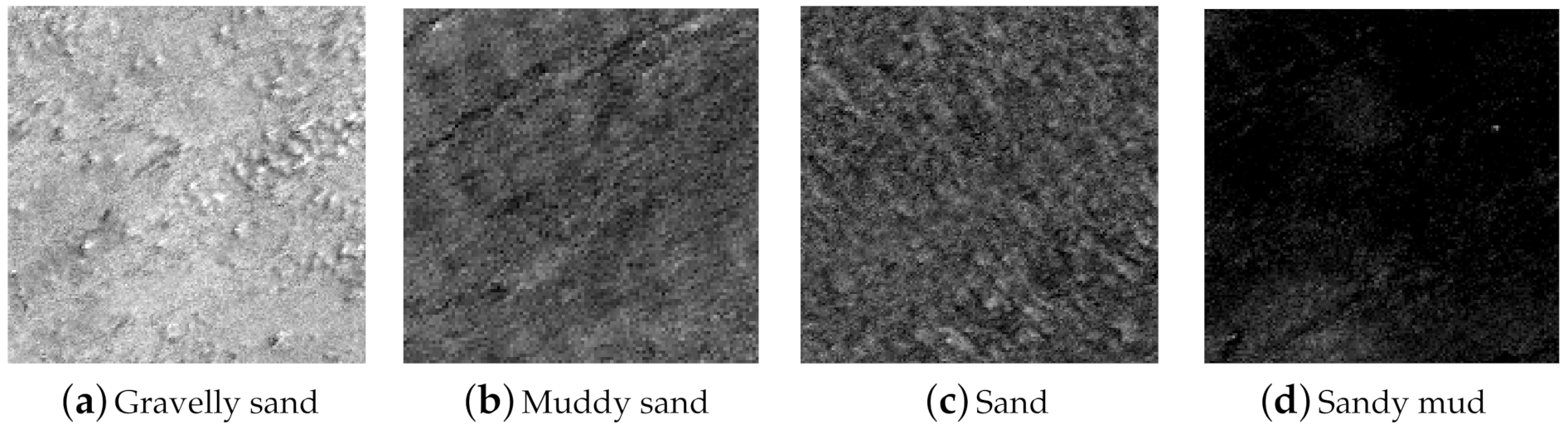
2.2. Ground-Truth Data Acquisition and Processing

The ground-truth data were collected by means of cylindrical box-core samples. This type of sampling gear conserves the surficial composition and configuration of the seafloor while conserving the subsurface stratigraphy, providing qualitative geotechnical appreciations of the nature of the sediment in the study area. Using the ternary sediment classification of Folk (1954), samples were labeled as Sand (S), Sandy mud (sM), Muddy sand (mS), and Gravelly sand (gS) as shown in Figure 3. Sediment categories were determined by a combination of particle size analysis (by means of a Malvern Mastersizer 3000) and expert visual observation. Overall, the ground-truth dataset consists of 19 samples and their locations are displayed using colored circular markers in Figure 2.

Figure 4 shows the probability density distribution for the backscatter and depth variation in the study area and the adopted sample datasets (Figure 4a,c). The probability density value is normalized between 0 and 1. The selected sample datasets adopted in the experiments have a similar density distribution both in backscatter intensity and depth, indicating that those samples represent the whole area well. The boxplot clearly shows that the samples from each type of sediment tend to have a particular backscatter region and depth zone (Figure 4b,d). “Training” and “test” refer to the distributions of the training and validation sample datasets used in the classification.

2.3. Seafloor Characterization Based on the Weyl Transform

Within the framework of ASC, MBES data are integrated with ground-truth data. As MBES backscatter data relates to seafloor surficial structure and composition, texture is regarded as one of the most efficacious features in image-based sediment mapping research. When dealing with the texture image classification tasks, we are interested in representations that are invariant under a given group of transformations, such as translation, scaling, and rotation. The Weyl transform has recently shown remarkable results in the context of texture classification with standard texture images [40], outperforming some common textural descriptors including Histograms of Oriented Gradients (HOG) [45] and Local Binary Pattern (LBP) [46]. HOG and LBP are very popular methods for texture description in computer vision, such as human detection and biomedical recognition problems. The Weyl transform is a mapping between a vectorized signal and its autocorrelation coefficients, which can capture multiscale symmetries of the texture. The transform has the desirable property of being invariant to a large class of multiscale signed permutations. In particular, different ways of orienting and translating the same texture will produce the same Weyl descriptor, and patches sampled from the same texture should share similar Weyl transforms.

2.3.1. The Weyl Representation

The Weyl transform distinguishes different textural structures by quantifying multiscale symmetry features [41]. Moreover, invariance to multiscale transformations ensures that image patches with the same textural structures result in similar Weyl representation. The binary Heisenberg-Weyl group $H{W}_{2^m}$ is a group of permutation matrices and matrices that resemble permutation matrices with sign changes in some of the rows. Those square matrices of size $2^m$ exist for each power of 2 and are defined as Kronecker products:

$$D(a,b)=D(a,0)D(0,b)=x^{a_{m-1}}{z}^{b_{m-1}}\otimes \cdots \otimes x^{a_0}{z}^{b_0},$$

(1)

where

$$x=\left[\begin{array}{cc}0& 1\\ 1& 0\end{array}\right],z=\left[\begin{array}{cc}1& 0\\ 0& -1\end{array}\right],$$

and $a=(a_0,\dots ,a_{m-1}),b=(b_0,\dots ,b_{m-1})\in {\mathbb{Z}}_2^m$ are two binary m-tuples. Formally, the binary Heisenberg-Weyl group $H{W}_{2^m}$ of order $2^{2m+2}$ is defined as $H{W}_{2^m}=\left\{i^{\lambda }D(a,b)\right|\lambda \in \{0,1,2,3\}\mathrm{and}a,b\in {\mathbb{Z}}_2^m\}.$

As shown in [40], the signed permutation matrices $D(a,b)$ with $a^{T}b=0$ form an orthonormal basis of the vector space of real square symmetric matrices with respect to the inner product given by $\langle R,S\rangle :=\mathrm{tr}\left(R^{T}S\right).$ In particular, each real symmetric matrix R can be represented as a linear combination of the basis elements as

$$\begin{array}{c}\hfill R=\sum _{\begin{array}{c}a,b\in {\mathbb{Z}}_2^m\\ a{b}^T=0\end{array}}\left\{\frac{1}{2^{m/2}}\mathrm{tr}\left[R·D(a,b)\right]\right\}\frac{1}{2^{m/2}}D(a,b).\end{array}$$

(2)

Given a vectorized signal $y\in {\mathbb{R}}^{2^m}$, its covariance matrix $y{y}^T\in {\mathbb{R}}^{2^m\times 2^m}$ is a real symmetric matrix and as such can be represented as

$$\begin{array}{c}\hfill \begin{array}{cc}\hfill y{y}^T=& \sum _{\genfrac{}{}{0pt}{}{a,b\in {\mathbb{Z}}_2^m}{a{b}^T=0}}\left\{\frac{1}{2^{m/2}}tr\left[y{y}^T·D(a,b)\right]\right\}\frac{1}{2^{m/2}}D(a,b)\hfill \\ \hfill =& \sum _{\genfrac{}{}{0pt}{}{a,b\in {\mathbb{Z}}_2^m}{a{b}^T=0}}{\omega }_{a,b}\left(y\right)\frac{1}{2^{m/2}}D(a,b).\hfill \end{array}\end{array}$$

(3)

Coefficients ${\omega }_{a,b}\left(y\right)$ are the Weyl coefficients of the signal y and the corresponding isometric mapping $y{y}^T\mapsto {\omega }_{a,b}\left(y\right)$ is the Weyl transform [40]. Each vector y can be indexed by a binary m-tuple $v={(v_{m-1}\dots v_0)}^T$. The covariance matrix $y{y}^T$ can be regarded as a combination of multiple autocorrelation bands and an autocorrelation band of y can be represented as $z_a\in {\mathbb{R}}^{2^m}$, where

$$\begin{array}{c}\hfill {\left(z_a\right)}_v:=y_v{y}_{v+a}.\end{array}$$

(4)

Let ${\omega }_a\in {\mathbb{R}}^{2^m}$ represent a subset of Weyl coefficients labeled by a m-tuple a, defined by ${\left({\omega }_a\right)}_b:={\omega }_{a,b}$. Given binary m-tuples v and w, Walsh–Hadamard transform matrix can be defined as

$$\begin{array}{c}\hfill {\left(H_{2^m}\right)}_{v,w}:=\frac{1}{2^{m/2}}{(-1)}^{v^{T}w}.\end{array}$$

(5)

It results in ${\omega }_a\left(y\right)=H_{2^m}{z}_a$, where ${\left\{{\omega }_a\right\}}_b=0$ if $a^{T}b=1$. This implies that the Weyl transform can be seen as the Walsh–Hadamard transform of binary autocorrelations.

The absolute values of the Weyl transform coefficients are invariant under conjugation by any element of the binary Weyl-Heisenberg group $D_{a,b}$ as well as by left or right multiplication by $D_{a,b}$. Moreover, the values are invariant under conjugation by a larger group of permutations corresponding to elements of the binary symplectic group $\mathrm{Sp}(2m,\mathbb{Z})$.

2.3.2. Texture Descriptor

MBES backscatter data record quantitatively acoustic intensity scattered to the underwater transducer from the seafloor. Through a series of data processing stages, the backscatter strengths are processed into sedimentologically meaningful relative backscatter level, which subsequently serves as the source data to be mapped into image pixels using an appropriate grid resolution and a reasonable resampling strategy [9]. We hypothesize that autocorrelation, and especially the dyadic autocorrelation framework from Section 2.3.1, can provide good discrimination between greyscale patterns corresponding to different sediment types. Hence, we design here a texture descriptor based on the Weyl transform to represent the local pattern of the backscatter mosaic as concomitant characteristics relating to seafloor physical property.

We divide the multibeam backscatter image into relatively small patches using a moving window of size $S_w\times S_w$ ($S_w=2^r,r\in {\mathbb{Z}}^{+}$) (the effect of the patch size is analyzed in Section 2.5), with a sliding step of $S_t$. Each patch can be vectorized in a raster-scanning fashion which results in a $S=2^{2r}$ dimensional vector. Let $m=2r$, $a={(a_{m-1}\dots a_0)}^T$ and $b={(b_{m-1}\dots b_0)}^T$. Then, the Weyl coefficients of patch Y are computed by using Equation (3). Figure 5 shows how we obtain the Weyl representation of a selected patch from a multibeam backscatter image. The complete procedure of the Weyl coefficients computation is summarized in Algorithm 1.

Algorithm 1: Weyl feature extraction from multibeam backscatter images.

Input:    A multibeam backscatter image, sampling size $S_w$, sliding step $S_t$ Procedures:     1: Extract an image patch from the whole image using a moving window of size $S_w\times S_w$.     2: Vectorize the selected patch by stacking all pixels, resulting in a vector $y\in {\mathbb{R}}^{2^m}$.     3: Compute the covariance matrix $y{y}^T\in {\mathbb{R}}^{2^m\times 2^m}$.     4: Generate a collection of signed permutation matrices $D(a,b)\in {\mathbb{R}}^{2^m\times 2^m}$, $a,b\in {\mathbb{Z}}_2^m$.     5: Calculate the Weyl coefficients ${\omega }_{a,b}$ using the Equation (3). Output:    Weyl coefficients of the image patch

2.4. Cluster Consistency Comparison with Classical Texture Features

In an ideal classification problem scenario, an optimal textural descriptor should maximize the interclass variability while minimizing the intraclass variability (the same principle applies to the goal of the classification itself; the textural feature enhances this possibility). To evaluate this process in a simplified scenario, 19 blocks were identified within the backscatter image of the surveyed area, being centered with box-core samples and including a very limited area around their neighborhoods (with an area of $256\times 256\mathrm{m}$). Figure 6 shows four backscatter blocks centered with different sediment types. Based on prior knowledge and data analysis, the block size is determined by manual interpretation. We assumed that each block displays a representative and consistent backscatter image texture. We made another assumption that patches from a block belonged to the same class of sediment (these two assumptions are referred to as neighborhood consistency). Then, the locations selected were of a known sediment type, from the ground-truth points. It must be clarified that the relatively small number of ground-truth datapoints available in this investigation may pose a risk to the neighborhood consistency assumptions put forward. Therefore, randomness in image block selection is counteracted by repeating experiments, whereas autocorrelation is treated by introducing a spatial blocking strategy in the image sampling process. For each of the four sediment categories, we randomly sampled 500 $8\times 8$ patches from the backscatter image in the blocks, with a total of 2000 samples. In turn, these samples were used to derive (a) first-order statistics (FOS), (b) GLCM features, (c) wavelet coefficients (WLT), (d) LBP features and (e) Weyl coefficients (WT). First-order statistics contained five features derived from greyscale imagery, including maximum, minimum, mean, variance, and mode. Statistical features derived from GLCM included contrast, correlation, entropy, homogeneity, and angular second moment. Wavelet coefficients were extracted by performing a level one decomposition using Daubechies wavelet (db2), containing mean and standard deviation of one approximation coefficient and three detail coefficients. LBP encoded local texture structures as normalized histograms using ${\ell }_1$ norm. The Weyl coefficients were calculated using Algorithm 1.

In order to quantitatively state the cohesion and separation of the sample clusters in each feature space, the silhouette index (SI) was introduced to access the data consistency within clusters [47]. The silhouette value is a measure of how similar an object is to its own cluster (cohesion) compared to other clusters (separation). The silhouette index is calculated using the mean intracluster distance and the mean nearest-cluster distance (Euclidean distance) for each sample. The silhouette validation technique calculates the silhouette index for each sample, average silhouette index for each cluster and overall average silhouette index for a dataset. After the dimension reduction, a series of x, y, z cartesian plots will aid the visualization of the cluster discrimination potential and separation for those feature extraction methods above at multiple scales. SI computation and all feature extraction methods were implemented using built-in functions in MATLAB R2020b (64-bit) on a computer with an Intel^® Core ${}^{\mathrm{TM}}$ i7-7700HQ CPU.

2.5. Scale Selection

In this research, we evaluated the effect of the scale of the Weyl coefficients on MBES backscatter imagery so that the relative results can aid the selection of an optimal scale factor to carry out and improve the performance of image-based ASC. To appraise the effect of scale on the sediment type discrimination potential, the following patch sizes were selected for neighborhood analysis: $4\times 4$, $8\times 8$, $16\times 16$, $32\times 32$ pixels. For each selected scale and for each of the five feature derivation methods, 2000 image patches (for each sediment type, 500 patches sampled in the same way as the cluster consistency test) were obtained and plotted in a reduced dimensional space obtained by means of Principle Component Analysis (PCA).

2.6. Statistical Modeling and Protocol of Error Estimation

To validate the performance of the proposed texture descriptor based on the Weyl transform, we employed an Random Forest (RF) as a classifier for the purpose of quantitative comparison [48]. We implemented the routine in Python 3.8 (64-bit) using the module of sklearn.ensemble. In the training process of the model, parameters were set as follows: the number of trees in the forest was 100 (more trees did not significantly improve the model performance in the test), the number of features to consider when looking for the best split was the square root of the number of all features, Gini impurity was used to measure the quality of a split, bootstrap samples were used when building trees, and the other parameters were left as default.

In general, seafloor data are spatially autocorrelated, which means that those observations close to each other are more similar than distant ones. To avoid the problem of spatial autocorrelation in the sampling data, we adopted a spatial blocking strategy for the allocation of samples to training set and test set. In each identified block of the whole backscatter image, we split the backscatter data spatially into several subblocks. The checkerboard pattern is adopted for the allocation of subblocks to two different folds. This strategy can avoid adjacent subblocks in a fold, which means that all samples of the test set are excluded from the training set [49]. For each subblock, we took $8\times 8$ patches by overlapping sampling with a sliding step of 4 pixels, with 32,400 samples being available in total both in training set and test set. In the experiments, we randomly took 2000 samples for every class of the sediment from the dataset, including backscatter patches and their corresponding labels. The training set contained 200 samples and the test set contained the other 1800 of the samples. To quantitatively validate the performance of the proposed texture descriptor for acoustic sediment classification, we performed sediment classification on the test set by feeding the feature variables to a trained RF model using the training set. In the results, each test patch was assigned to a sediment category by a majority voting from the various individual trees in the RF model.

The protocol of error estimation was based on derivation of accuracy metrics from the confusion matrix [50]. The confusion matrix cross tabulates predicted and observed instances providing information on the correct allocation of class labels (along the matrix diagonal) and of class labels confusion between categories (over the offdiagonal entries). The derived metrics included: Overall Accuracy ($A_o$) (defined by the number of overall correctly allocated instances divided from the overall number of validation samples), Cohen’s Kappa (K) (also referred to as “chance agreement”), Recall Rate (R) (the true positive rate) and the OOB RF error ($ER$) (the error rate estimated by about 36.8% of samples withheld from the training dataset).

3. Experimental Results

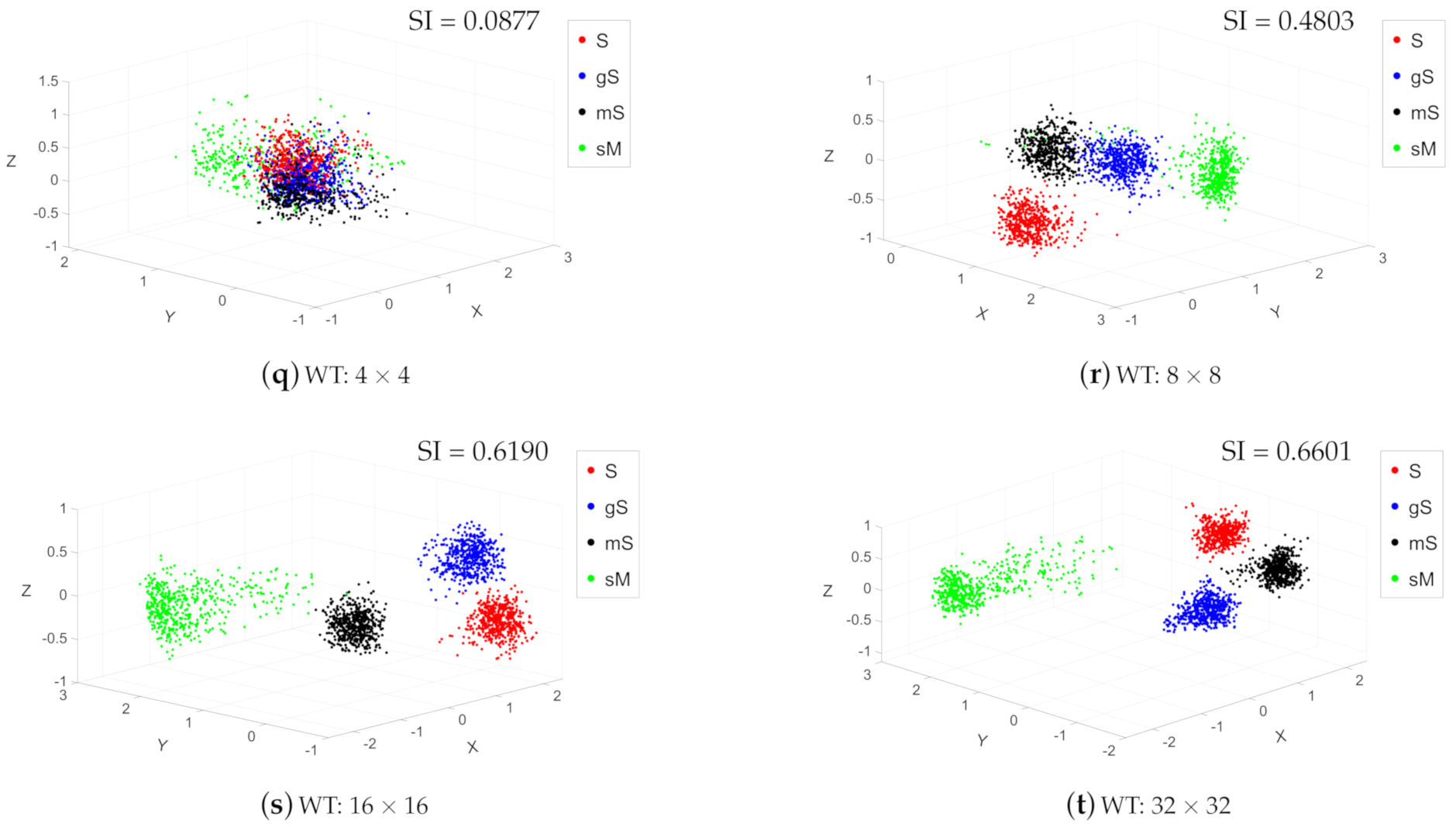
3.1. Clustering Analysis

Figure 7 shows the x, y, z scatter plots for the various features to aid the visualization, and each feature space is projected into three dimensions using PCA. Datapoints are color-coded according to the sediment category: gS (blue), mS (black), sM (green), S (red). Of the traditional features in the same scale of $8\times 8$, the “First-order Statistics” method (Figure 7b) produced the sharpest cluster separation, with two isolated clusters (blue and green) and one overlapping area (between black and red). The approaches “GLCM” (Figure 7f) and “Wavelet Transform” (Figure 7j) produced moderate separations, both with two overlaps in the outer area of the clusters. “LBP” (Figure 7n) is not able to generate separated clusters for these four classes of samples. Figure 7r shows the potential of the Weyl transform compared to the other set of features (Figure 7b,f,j,n), which presents tight aggregation and clear boundary. To enable a quantitative assessment, the silhouette indexes were calculated for the samples in all feature spaces (

Table 1. Silhouette index of five feature spaces in different spatial scales for four clusters.

Silhouette Index	Scale	$4\times 4$	$8\times 8$	$16\times 16$	$32\times 32$
Method
First-order statistics		0.3963	0.4386	0.5202	0.6301
GLCM features		0.3126	0.3880	0.4454	0.6213
Wavelet transform		0.2248	0.3373	0.3763	0.4207
LBP		−0.0175	0.0578	0.3449	0.4480
Weyl transform		0.0877	0.4803	0.6190	0.6601

): the Weyl coefficients obtained 0.4803, which was the highest in five features, while LBP gave the lowest value 0.0578. The other three methods provided moderate performance: 0.4386, 0.3880, 0.3373 respectively for first-order statistics, GLCM, and Wavelet transform.

3.2. Multiple Scale Analysis

The cluster separation potential resulting from the overall five feature derivation approaches is shown in Figure 7. These results clearly show how cluster separation varies as a function of spatial scale. It can be generally stated that increasing the scale increased the cluster separation for all approaches herein tested.

In the traditional methods, with a sampling size of smaller than $8\times 8$, samples represented by first-order statistics, GLCM features, and wavelet coefficients can cluster together for each class, but interclass distance was quite near and some of the clusters were partly overlapping in the outer edge. Samples represented using LBP features were mixed for all four classes. Only when the sampling size was larger than $16\times 16$, those traditional methods can show satisfied discriminability, with slight or no overlap areas. Regarding the Weyl coefficients, Figure 7q–t), with increasing the sampling scale, the clusters become more compact, and the overlap areas between clusters become smaller. Intermediate values of scale (i.e., $8\times 8$) were sufficient to isolate distinct clusters, and all the values of scale larger than $8\times 8$ produced sharp cluster separation.

Table 1 quantitatively shows the tendency of the sample distributions by different features and scales using silhouette values of the resulting clusters. We can see that silhouette value increases as the scale increasing in each row of the table. In the column of $4\times 4$, first-order statistics obtained the highest silhouette index, while the Weyl transform achieved the highest value in the scales of $8\times 8$, $16\times 16$ and $32\times 32$.

Figure 7. Discriminability of five feature extraction methods in four scales.

Figure 7. Discriminability of five feature extraction methods in four scales.

3.3. Quantitative Comparison of Classification Accuracy

We compared the performance of the five feature derivation approaches and the detailed classification results using different approaches are reported in

Table 2. Classification results of the Random Forest model using first-order Statistics.

	Prediction	S	gS	mS	sM	Total	Accuracy	K	$\mathit{ER}$
Ground-Truth
S		809	612	352	27	1800	44.94%	0.6120	28.50%
gS		572	1212	16	0	1800	67.33%
mS		264	72	1456	8	1800	80.89%
sM		43	0	129	1628	1800	90.44%
Total		1688	1896	1953	1663	7200	70.90%

,

Table 3. Classification results of the Random Forest model using Gray Level Co-occurrence Matrices features.

	Prediction	S	gS	mS	sM	Total	Accuracy	K	$\mathit{ER}$
Ground-Truth
S		761	640	380	19	1800	42.28%	0.6057	29.75%
gS		508	1260	31	1	1800	70.00%
mS		296	61	1433	10	1800	79.61%
sM		47	0	136	1617	1800	89.83%
Total		1612	1961	1980	1647	7200	70.43%

,

Table 4. Classification results of the Random Forest model using Wavelet Transform.

	Prediction	S	gS	mS	sM	Total	Accuracy	K	$\mathit{ER}$
Ground-Truth
S		710	656	395	39	1800	39.44%	0.6217	28.13%
gS		434	1337	29	0	1800	74.28%
mS		236	103	1441	20	1800	80.06%
sM		22	0	109	1669	1800	92.72%
Total		1402	2096	1974	1728	7200	71.63%

,

Table 5. Classification results of the Random Forest model using Local Binary Pattern.

	Prediction	S	gS	mS	sM	Total	Accuracy	K	$\mathit{ER}$
Ground-Truth
S		603	660	516	21	1800	33.50%	0.2276	59.13%
gS		639	608	535	18	1800	33.78%
mS		504	563	708	25	1800	39.33%
sM		176	213	301	1110	1800	61.67%
Total		1922	2044	2060	1174	7200	42.07%

and

Table 6. Classification results of the Random Forest model using the Weyl Transform.

	Prediction	S	gS	mS	sM	Total	Accuracy	K	$\mathit{ER}$
Ground-Truth
S		1358	425	17	0	1800	75.44%	0.7119	21.25%
gS		517	1108	169	6	1800	61.56%
mS		38	328	1412	22	1800	78.44%
sM		0	11	23	1766	1800	98.11%
Total		1913	1872	1621	1794	7200	78.39%

. First-order statistics, GLCM features, and wavelet coefficients all demonstrated a superior classification accuracy for Muddy sand and Sandy mud as compared with Sand and Gravelly sand. The overall accuracies of these three methods were at the same level, which are respectively 70.90%, 70.43%, and 71.63%. LBP produced the poorest recall rates for all classes and the lowest overall accuracy. The Weyl transform achieved the best overall classification accuracy. To be specific, higher classification accuracies were obtained for Sand, Muddy sand, and Sandy mud as compared with Gravelly sand. It should be noted that recall rates of all classes in the Weyl transform were above 61%, which none of the other approaches achieved. In order to avoid the biased classification results by randomness, we present the averaged performance of each method for recognizing four classes of sediment in

Table 7. Mean accuracy of the Random Forest model with different features by running 10 tests.

Method	Classification Accuracy
	S	gS	mS	sM	Total	${\mathit{A}}_{\mathit{o}}$
First-order statistics	43.36%	69.91%	77.33%	92.16%	7200	70.69%
GLCM features	40.05%	71.21%	75.29%	91.57%	7200	69.53%
Wavelet transform	37.46%	74.26%	77.56%	92.28%	7200	70.39%
LBP	38.17%	31.01%	38.36%	62.69%	7200	42.56%
Weyl transform	62.49%	62.13%	86.18%	96.61%	7200	76.85%

after running the test 10 times. The recall rates of each class are presented in the first four columns in Table 7, and the mean overall accuracy of the test is presented in the last column. The overall accuracy scores show that the Weyl coefficients outperformed both single feature extraction methods ($A_o$ reaching 76.85%). The Weyl transform achieved both a high overall accuracy as well as high by-class accuracy scores for the classes Sand, Muddy sand, and Sandy mud. Especially, the Weyl transform significantly improves the classification accuracy of the class Sand, which otherwise produced the lowest accuracy scores in the other tested feature derivation approaches (Figure 8).

4. Discussion

In the context of predictive modeling for acoustic seafloor classification, feature derivation enhances the characteristics of the primary data (i.e., its variability), ultimately improving the classification problem. The goal of the derived feature is that of maximising within-class homogeneity and between-class variability. The derivation of secondary features is particularly appealing where the classification task requires the fitting of a prescribed classification scheme over acoustic data with limited sediment discrimination potential, as for the Folk classes herein tested with 300 kHz MBES backscatter data (with respect to the acoustical operating frequency) [51]. In the projected 3-D feature space, compactness and overlap (i.e., consistency) of the clusters (quantified by the associated metrics, i.e., silhouette coefficients) are retained as key indicators for the evaluation of a feature’s classification performance. Recognizing the importance of feature extraction in acoustic seafloor classification, this experimental investigation proposed the Weyl transform as a novel texture-based descriptor of MBES compensated backscatter imagery. This feature enhances thematic cluster separation in terms of Folk (1954) sedimentological categories. Experiments were dedicated to both visually and quantitatively comparing and evaluating thematic cluster consistency across five reduced feature derivation approaches (herein referred to as “traditional features” and dimensionally reduced by PCA) and across various scales of derivation (i.e., neighborhood/window sizes). Furthermore, comparative analyses were set up to evaluate the thematic predictive accuracy of random forest models based on the five disparate sets of secondary features. Together, the experimental results converged showing that based on the backscatter dataset herein used, the texture-based Weyl transform outperformed the other secondary features traditionally used in seafloor sediment classification.

4.1. Multiscale Cluster Consistency

Reduced dimensional space plots (Figure 7), produced for multiple window scales (i.e., $4\times 4$, $8\times 8$, $16\times 16$ and $32\times 32$), allowed observing different behaviors of the tested approaches. Visually, inspecting the cluster compactness in the 3D space revealed that LBP, first-order statistics, GLCM, and wavelet transform approaches all resulted in substantially overlapping clusters, across all scales assessed for, hence leading to misclassification in the subsequent stage and hindering the prediction of the categories in geographical space (see Section 4.2 in the discussion). In contrast, the Weyl transform produced the sharpest clusters, showing clear separation of the four prescribed categories at all scales except for the smallest windows sizes ($4\times 4$). Noticeably, across all approaches tested, the multiscale cluster consistency analysis (summarized in Table 1 by means of Silhouette coefficients), indicated that cluster separation increased with increasing window size, reaching the highest separation scores for the $32\times 32$ window size. While this suggests a potentially well-performing classification using these features at such a scale, it would come at the cost of losing spatial information, contrasting to the objective of high-resolution seafloor sediment mapping. This behavior, and subsequent limitation, is attributed to the window size: until a size of $32\times 32$, it is unable to produce a histogram representative of the statistical distribution of the grey levels for that given thematic class. The Weyl transform produced the highest silhouette scores, outperforming all other approaches in terms of compactness and separation for the representation of these sediment categories. The multiscale cluster consistency analysis identified $8\times 8$ as the optimal scale for the Weyl transform. This indicates that the Weyl transform requires less information (a smaller sampling size) than the traditional approaches tested. However, it is important to note that this may be a dataset-specific result, requiring further testing on different backscatter and ground-truth datasets. The optimal scale for analysis closely relates to the practical geological conditions and it would constantly vary with the characteristics of the seafloor. The fact that the Weyl transform coefficients achieve high separability performance with a smaller sampling size is indeed a desirable result.

4.2. Classification Accuracy

Once the optimal scale and the desirable properties of the Weyl transform were appraised, the investigation looked at the thematic classification accuracy of random forest models built on the different feature derivation approaches. Here, the Weyl transform achieved the best performance in terms of overall classification accuracy. First-order statistics, GLCM features, and wavelet coefficients scored similar overall accuracies, ranking second to the Weyl transform. LBP showed the lowest performance. Classification accuracy was also appreciated based on by-class accuracies, indicating that compared to other models, the Weyl transform improves the prediction of three out of four types of sediment (Sand, Muddy sand, and Sandy mud). This mainly results from the invariance to a large class of multiscale dihedral transformations. A collection of signed permutation matrices provides good capability for describing textures, with the high-order terms giving coarse-scale permutations and the low-order terms giving fine-scale permutations. The Weyl transform can capture multiscale symmetries that are important in identifying textural structures from acoustical images and associate those with sediment categories. This ensures that the Weyl coefficients of the backscatter image patches obtained from the same sediment type exhibit similarity [40]. Only the category Gravelly sand achieved lower accuracies. The classification accuracy of all classes may be improved by enlarging the sampling window size. However, this would inevitably represent a trade-off: decreasing resolution to increase accuracy. Indeed, several methodological comparative studies, including this investigation, suggest that, to date, there exists no single methodological routine that can consistently achieve the best classification performance, and hybrid approaches, such as ensemble and combinatory maps, integrating into one product the best performing parts of multiple models, has been proposed as a possible way forward [3,25,28]. Similarly, with respect to feature extraction, one possible way forward is that of developing deep feature fusion methods: an approach by which various features are recombined to reach their fullest discrimination potential capabilities [52,53,54]. Recent marine habitat mapping studies by Janowski et al. (2018) confirm that for a dataset with an overlapping distribution of backscatter intensities between classes, secondary features derived from MBES data can substantially contribute to classification prediction accuracy [55]. Therefore, this suggests that rather than relying on an ensemble map, refinements at the ASC pipeline stage of the feature extraction could largely benefit classification performance.

5. Conclusions

In this investigation, the Weyl transform was introduced as a novel texture-based descriptor of MBES backscatter imagery, specifically as an aid to its classification into sediment categories that are at the center of attention of European seafloor sediment mapping harmonisation efforts (i.e., https://www.emodnet-geology.eu/map-viewer/?p=seabed_substrate [56] (accessed on 10 December 2020). The texture descriptor based on the Weyl coefficients describes effectively the multiscale correlation features resulting from MBES backscatter images. The importance of multiscale assessments to avoid the arbitrary selection of the scale parameter was confirmed. Overall and by-class classification accuracy metrics demonstrated that the Weyl transform can improve model accuracy based on the tested dataset and under the spatial assumptions of neighborhood consistency put forward in the methodology. Besides the favorable characteristics of the Weyl transform, no single feature could achieve the best predictive classification performance for all the sediment categories. Feature fusion, similar to hybrid mapping methods merging the outputs of disparate classifiers, shall be explored as a further way of improving classification. Further research is needed to elucidate the physical relationship between scale, Weyl transform, and sediment classes, including testing the method on different backscatter and ground-truth datasets and habitat classification schemes.

References

1. Halpern, B.S.; Walbridge, S.; Selkoe, K.A.; Kappel, C.V.; Micheli, F.; D’Agrosa, C.; Bruno, J.F.; Casey, K.S.; Ebert, C.; Fox, H.E.; et al. A global map of human impact on marine ecosystems. Science 2008, 319, 948–952. [Google Scholar] [CrossRef] [Green Version]
2. Douvere, F. The importance of marine spatial planning in advancing ecosystem-based sea use management. Mar. Policy 2008, 32, 762–771. [Google Scholar] [CrossRef]
3. Diesing, M.; Mitchell, P.J.; O’Keeffe, E.; Gavazzi, G.O.A.M.; Bas, T.L. Limitations of Predicting Substrate Classes on a Sedimentary Complex but Morphologically Simple Seabed. Remote Sens. 2020, 12, 3398. [Google Scholar] [CrossRef]
4. Kostylev, V.E.; Todd, B.J.; Fader, G.B.; Courtney, R.; Cameron, G.D.; Pickrill, R.A. Benthic habitat mapping on the Scotian Shelf based on multibeam bathymetry, surficial geology and sea floor photographs. Mar. Ecol. Prog. Ser. 2001, 219, 121–137. [Google Scholar] [CrossRef] [Green Version]
5. McArthur, M.; Brooke, B.; Przeslawski, R.; Ryan, D.; Lucieer, V.; Nichol, S.; McCallum, A.; Mellin, C.; Cresswell, I.; Radke, L.C. On the use of abiotic surrogates to describe marine benthic biodiversity. Estuar. Coast. Shelf Sci. 2010, 88, 21–32. [Google Scholar] [CrossRef]
6. Kenny, A.; Cato, I.; Desprez, M.; Fader, G.; Schüttenhelm, R.; Side, J. An overview of seabed-mapping technologies in the context of marine habitat classification. ICES J. Mar. Sci. 2003, 60, 411–418. [Google Scholar] [CrossRef] [Green Version]
7. Lurton, X.; Augustin, J. A Measurement Quality Factor for Swath Bathymetry Sounders. IEEE J. Ocean. Eng. 2010, 35, 852–862. [Google Scholar] [CrossRef]
8. Lurton, X.; Lamarche, G.; Brown, C.; Lucieer, V.; Rice, G.; Schimel, A.; Weber, T. Backscatter Measurements by Seafloor-Mapping Sonars. Guidelines and Recommendations. Available online: http://geohab.org/wp-content/uploads/2014/05/BSWGREPORT-MAY2015.pdf (accessed on 7 January 2020).
9. Schimel, A.C.G.; Beaudoin, J.; Parnum, I.M.; Le Bas, T.; Schmidt, V.; Keith, G.; Ierodiaconou, D. Multibeam sonar backscatter data processing. Mar. Geophys. Res. 2018, 39, 121–137. [Google Scholar] [CrossRef]
10. Brown, C.J.; Todd, B.J.; Kostylev, V.E.; Pickrill, R.A. Image-based classification of multibeam sonar backscatter data for objective surficial sediment mapping of Georges Bank, Canada. Cont. Shelf Res. 2011, 31, S110–S119. [Google Scholar] [CrossRef]
11. Montereale Gavazzi, G.; Madricardo, F.; Janowski, L.; Kruss, A.; Blondel, P.; Sigovini, M.; Foglini, F. Evaluation of seabed mapping methods for fine-scale classification of extremely shallow benthic habitats-Application to the Venice Lagoon, Italy. Estuar. Coast. Shelf Sci. 2016, 170, 45–60. [Google Scholar] [CrossRef] [Green Version]
12. Gaida, T.C.; Snellen, M.; van Dijk, T.A.G.P.; Simons, D.G. Geostatistical modelling of multibeam backscatter for full-coverage seabed sediment maps. Hydrobiologia 2018. [Google Scholar] [CrossRef] [Green Version]
13. Mayer, L.; Jakobsson, M.; Allen, G.; Dorschel, B.; Falconer, R.; Ferrini, V.; Lamarche, G.; Snaith, H.; Weatherall, P. The Nippon Foundation—GEBCO Seabed 2030 Project: The Quest to See the World’s Oceans Completely Mapped by 2030. Geosciences 2018, 8, 63. [Google Scholar] [CrossRef] [Green Version]
14. Collier, J.S.; Brown, C.J. Correlation of sidescan backscatter with grain size distribution of surficial seabed sediments. Mar. Geol. 2005, 214, 431–449. [Google Scholar] [CrossRef]
15. Ferrini, V.L.; Flood, R.D. The effects of fine-scale surface roughness and grain size on 300 kHz multibeam backscatter intensity in sandy marine sedimentary environments. Mar. Geol. 2006, 228, 153–172. [Google Scholar] [CrossRef]
16. Goff, J.A.; Kraft, B.J.; Mayer, L.A.; Schock, S.G.; Sommerfield, C.K.; Olson, H.C.; Gulick, S.P.S.; Nordfjord, S. Seabed characterization on the New Jersey middle and outer shelf: Correlatability and spatial variability of seafloor sediment properties. Mar. Geol. 2004, 209, 147–172. [Google Scholar] [CrossRef]
17. Lamarche, G.; Lurton, X. Recommendations for improved and coherent acquisition and processing of backscatter data from seafloor-mapping sonars. Mar. Geophys. Res. 2018, 39, 5–22. [Google Scholar] [CrossRef] [Green Version]
18. Fonseca, L.; Mayer, L. Remote estimation of surficial seafloor properties through the application Angular Range Analysis to multibeam sonar data. Mar. Geophys. Res. 2007, 28, 119–126. [Google Scholar] [CrossRef]
19. Anderson, J.T.; Holliday, V.; Kloser, R.; Reid, D.; Simard, Y.; Brown, C.J.; Chapman, R.; Coggan, R.; Kieser, R.; Michaels, W.L. Acoustic Seabed Classification of Marine Physical and Biological Landscapes. In Proceedings of the International Council for the Exploration of the Sea, Copenhagen, Denmark, August 2007; pp. 61–63. [Google Scholar]
20. Anderson, J.T.; Van Holliday, D.; Kloser, R.; Reid, D.G.; Simard, Y. Acoustic seabed classification: Current practice and future directions. ICES J. Mar. Sci. 2008, 65, 1004–1011. [Google Scholar] [CrossRef]
21. Stephens, D.; Diesing, M. A Comparison of Supervised Classification Methods for the Prediction of Substrate Type Using Multibeam Acoustic and Legacy Grain-Size Data. PLoS ONE 2014, 9, e93950. [Google Scholar] [CrossRef]
22. Gazis, I.Z.; Schoening, T.; Alevizos, E.; Greinert, J. Quantitative mapping and predictive modeling of Mn nodules’ distribution from hydroacoustic and optical AUV data linked by random forests machine learning. Biogeosciences 2018, 15, 7347–7377. [Google Scholar] [CrossRef] [Green Version]
23. Janowski, L.; Trzcinska, K.; Tegowski, J.; Kruss, A.; Rucinska-Zjadacz, M.; Pocwiardowski, P. Nearshore benthic habitat mapping based on multi-frequency, multibeam echosounder data using a combined object-based approach: A case study from the Rowy site in the southern Baltic sea. Remote Sens. 2018, 10, 1983. [Google Scholar] [CrossRef] [Green Version]
24. Ierodiaconou, D.; Schimel, A.C.G.; Kennedy, D.; Monk, J.; Gaylard, G.; Young, M.; Diesing, M.; Rattray, A. Combining pixel and object based image analysis of ultra-high resolution multibeam bathymetry and backscatter for habitat mapping in shallow marine waters. Mar. Geophys. Res. 2018, 39, 271–288. [Google Scholar] [CrossRef]
25. Porskamp, P.; Rattray, A.; Young, M.; Ierodiaconou, D. Multiscale and Hierarchical Classification for Benthic Habitat Mapping. Geosciences 2018, 8, 119. [Google Scholar] [CrossRef] [Green Version]
26. Turner, J.A.; Babcock, R.C.; Hovey, R.; Kendrick, G.A. Can single classifiers be as useful as model ensembles to produce benthic seabed substratum maps? Estuar. Coast. Shelf Sci. 2018, 204, 149–163. [Google Scholar] [CrossRef]
27. McLaren, K.; McIntyre, K.; Prospere, K. Using the random forest algorithm to integrate hydroacoustic data with satellite images to improve the mapping of shallow nearshore benthic features in a marine protected area in Jamaica. Giscience Remote Sens. 2019, 56, 1065–1092. [Google Scholar] [CrossRef]
28. Zelada Leon, A.; Huvenne, V.A.I.; Benoist, N.M.A.; Ferguson, M.; Bett, B.J.; Wynn, R.B. Assessing the Repeatability of Automated Seafloor Classification Algorithms, with Application in Marine Protected Area Monitoring. Remote Sens. 2020, 12, 1572. [Google Scholar] [CrossRef]
29. Haralick, R.M.; Shanmugam, K.; Dinstein, I.H. Textural features for image classification. IEEE Trans. Syst. Man Cybern. 1973, SMC-3, 610–621. [Google Scholar] [CrossRef] [Green Version]
30. Alevizos, E.; Snellen, M.; Simons, D.G.; Siemes, K.; Greinert, J. Acoustic discrimination of relatively homogeneous fine sediments using Bayesian classification on MBES data. Mar. Geol. 2015, 370, 31–42. [Google Scholar] [CrossRef]
31. Pace, N.G.; Dyer, C.M. Machine Classification of Sedimentary Sea Bottoms. IEEE Trans. Geosci. Electron. 1979, 17, 52–56. [Google Scholar] [CrossRef]
32. Huvenne, V.A.I.; Blondel, P.; Henriet, J.P. Textural analyses of sidescan sonar imagery from two mound provinces in the Porcupine Seabight. Mar. Geol. 2002, 189, 323–341. [Google Scholar] [CrossRef] [Green Version]
33. Huseby, R.B.; Milvang, O.; Solberg, A.S.; Bjerde, K.W. Seabed classification from multibeam echosounder data using statistical methods. In Proceedings of the OCEANS ’93, Victoria, BC, Canada, 18–21 October 1993; pp. III/229–III/233. [Google Scholar]
34. Snellen, M.; Gaida, T.C.; Koop, L.; Alevizos, E.; Simons, D.G. Performance of Multibeam Echosounder Backscatter-Based Classification for Monitoring Sediment Distributions Using Multitemporal Large-Scale Ocean Data Sets. IEEE J. Ocean. Eng. 2018, 44, 1–14. [Google Scholar] [CrossRef] [Green Version]
35. Carmichael, D.; Linnett, L.; Clarke, S.; Calder, B. Seabed classification through multifractal analysis of sidescan sonar imagery. IEE Proc. Radar Sonar Navig. 1996, 143, 140–148. [Google Scholar] [CrossRef]
36. Preston, J. Automated acoustic seabed classification of multibeam images of Stanton Banks. Appl. Acoust. 2009, 70, 1277–1287. [Google Scholar] [CrossRef]
37. Reut, Z.; Pace, N.; Heaton, M. Computer classification of sea beds by sonar. Nature 1985, 314, 426–428. [Google Scholar] [CrossRef]
38. Atallah, L.N. Learning from Sonar Data for the Classification of Underwater Seabeds. Ph.D. Thesis, University of Oxford, Oxford, UK, 2005. [Google Scholar]
39. Karoui, I.; Fablet, R.; Boucher, J.M.; Augustin, J.M. Seabed Segmentation Using Optimized Statistics of Sonar Textures. IEEE Trans. Geosci. Remote Sens. 2009, 47, 1621–1631. [Google Scholar] [CrossRef]
40. Qiu, Q.; Thompson, A.; Calderbank, R.; Sapiro, G. Data Representation Using the Weyl Transform. IEEE Trans. Signal Process. 2016, 64, 1844–1853. [Google Scholar] [CrossRef] [Green Version]
41. Ahn, H.K.; Qiu, Q.; Bosch, E.; Thompson, A.; Robles, F.E.; Sapiro, G.; Warren, W.S.; Calderbank, R. Classifying Pump-Probe Images of Melanocytic Lesions Using the WEYL Transform. In Proceedings of the 2018 IEEE International Conference on Acoustics, Speech and Signal Processing (ICASSP), Calgary, AB, Canada, 15–20 April 2018; pp. 4209–4213. [Google Scholar]
42. Howard, S.D.; Calderbank, A.R.; Moran, W. The finite Heisenberg-Weyl groups in radar and communications. EURASIP J. Adv. Signal Process. 2006, 085685. [Google Scholar] [CrossRef] [Green Version]
43. Montereale Gavazzi, G. Development of Seafloor Mapping Strategies Supporting Integrated Marine Management: Application of Seafloor Backscatter by Multibeam Echosounders. Ph.D. Thesis, Ghent University, Gent, Belgium, 2019. [Google Scholar]
44. Montereale Gavazzi, G.; Roche, M.; Lurton, X.; Degrendele, K.; Terseleer, N.; Van Lancker, V. Seafloor change detection using multibeam echosounder backscatter: Case study on the Belgian part of the North Sea. Mar. Geophys. Res. 2018, 39, 229–247. [Google Scholar] [CrossRef]
45. Dalal, N.; Triggs, B. Histograms of oriented gradients for human detection. In Proceedings of the 2005 IEEE Computer Society Conference on Computer Vision and Pattern Recognition (CVPR’05), San Diego, CA, USA, 20–25 June 2005; pp. 886–893. [Google Scholar]
46. Heikkila, M.; Pietikainen, M. A texture-based method for modeling the background and detecting moving objects. IEEE Trans. Pattern Anal. Mach. Int. 2006, 28, 657–662. [Google Scholar] [CrossRef] [Green Version]
47. Rousseeuw, P.J. Silhouettes: A graphical aid to the interpretation and validation of cluster analysis. J. Comput. Appl. Math. 1987, 20, 53–65. [Google Scholar] [CrossRef] [Green Version]
48. Breiman, L. Random forests. Mach. Learn. 2001, 45, 5–32. [Google Scholar] [CrossRef] [Green Version]
49. Valavi, R.; Elith, J.; Lahoz-Monfort, J.J.; Guillera-Arroita, G.; Warton, D. BLOCKCV: An R package for generating spatially or environmentally separated folds for k-fold cross-validation of species distribution models. Methods Ecol. Evol. 2018, 10, 225–232. [Google Scholar] [CrossRef] [Green Version]
50. Congalton, R.G. Accuracy assessment and validation of remotely sensed and other spatial information. Int. J. Wildland Fire 2001, 10, 321–328. [Google Scholar] [CrossRef] [Green Version]
51. Strong, J.A.; Clements, A.; Lillis, H.; Galparsoro, I.; Bildstein, T.; Pesch, R. A review of the influence of marine habitat classification schemes on mapping studies: Inherent assumptions, influence on end products, and suggestions for future developments. ICES J. Mar. Sci. 2019, 76, 10–22. [Google Scholar] [CrossRef] [Green Version]
52. Kong, W.Z.; Hong, J.C.; Jia, M.Y.; Yao, J.L.; Gong, W.H.; Hu, H.; Zhang, H.G. YOLOv3-DPFIN: A Dual-Path Feature Fusion Neural Network for Robust Real-Time Sonar Target Detection. IEEE Sens. J. 2020, 20, 3745–3756. [Google Scholar] [CrossRef]
53. Asokan, A.; Anitha, J.; Patrut, B.; Danciulescu, D.; Hemanth, D.J. Deep Feature Extraction and Feature Fusion for Bi-Temporal Satellite Image Classification. Comput. Mater. Contin. 2021, 66, 373–388. [Google Scholar] [CrossRef]
54. Mu, C.; Liu, Y.; Liu, Y. Hyperspectral Image Spectral–Spatial Classification Method Based on Deep Adaptive Feature Fusion. Remote Sens. 2021, 13, 746. [Google Scholar] [CrossRef]
55. Janowski, Ł.; Tęgowski, J.; Nowak, J. Seafloor mapping based on multibeam echosounder bathymetry and backscatter data using Object-Based Image Analysis: A case study from the Rewal site, the Southern Baltic. Oceanol. Hydrobiol. Stud. 2018, 47, 248–259. [Google Scholar] [CrossRef]
56. Kaskela, A.M.; Kotilainen, A.T.; Alanen, U.; Cooper, R.; Green, S.; Guinan, J.; van Heteren, S.; Kihlman, S.; Van Lancker, V.; Stevenson, A. Picking up the pieces—Harmonising and collating seabed substrate data for European maritime areas. Geosciences 2019, 9, 84. [Google Scholar] [CrossRef] [Green Version]
Figure 1. Location of the survey area. All spatial data were projected in Universal Transverse Mercator (UTM) Zone 31 North with Datum World Geodetic System (WGS) 1984. The depth contours were made available from the Agency for Maritime Services and Coast–Coastal Division–Flanders Hydrography.
Remotesensing 13 01760 g001
Figure 2. Map of the study area with backscatter and bathymetry and the location of the sediment samples. The bathymetry map is overlaid with a hill-shade layer, in which the vertical exaggeration Z is set 2, the sun azimuthal illumination orientation is 315 and the altitude is 45.
Remotesensing 13 01760 g002
Figure 3. Photographic record of four sediment types.
Remotesensing 13 01760 g003
Figure 4. (a) Backscatter distribution in the study area and per sample dataset, (b) boxplot of the backscatter for each type of sediment; (c) depth distribution in the study area and per sample dataset; (d) boxplot of the depth for each type of sediment.
Remotesensing 13 01760 g004
Figure 5. Computation of the Weyl coefficients for a Multibeam Echosounder System (MBES) backscatter image. The selected patch is vectorized by stacking its columns. The Weyl transform is applied to the stacked patch, and the dimensionality of the resulting coefficient vector is reduced by merging equivalent transformations to yield the Weyl feature vector.
Remotesensing 13 01760 g005
Figure 6. Identified backscatter blocks of four sediment types.
Remotesensing 13 01760 g006
Figure 8. Classification accuracy of the five feature extraction methods.
Remotesensing 13 01760 g008