1. Introduction
5G technologies present a new paradigm to provide connectivity to vehicles, in support of high data rate services, complementing existing AMP communication standards [
1]. The 5G network has low latency, high throughput, and high reliability, which greatly enhances the richness and timeliness of the information transmitted by the car network, and also improves the technical value of the car network sensor [
2]. It provides the network foundation for cloud computing and edge computing. This makes it possible for models based on deep learning using in autonomous moving platforms (AMP) [
3].
Autonomous vehicles usually have sensors such as LIDAR and cameras. The monocular camera has the advantages of low price, rich information content, and small size, which can effectively overcome the many shortcomings of other sensors. Therefore, the use of monocular camera to obtain depth information has important research significance, and has gradually become one of the research hot spots in the field of computer vision [
4,
5].
The traditional depth estimation methods estimate depth scene by fusing information from different views. Structure from motion (SfM) or simultaneous localization and mapping (SLAM) is considered to be an effective method for estimating depth structures [
6]. Typical SLAM algorithms estimate the ego-motion and the depth of scene in parallel. However, this type of method is highly dependent on the matching of points. Therefore, mismatching and insufficient features will still have a significant impact on the results [
7].
In recent years, deep learning methods based on deep neural networks have triggered another wave in the field of computer vision. A large number of documents indicate that deep neural networks have played a huge role in various aspects of computer vision, including target recognition [
8] and target tracking [
9,
10]. Traditional computer vision problems such as image segmentation have greatly improved in efficiency and accuracy. In the field of depth estimation, traditional methods based on multi-view geometry and methods based on machine learning have formed their respective theories and method systems. Therefore, researchers began to try to combine traditional computer vision methods with deep learning. Using deep learning methods to estimate the depth of the scene from a single picture is one of the important research directions [
11]. Compared with the traditional method based on multi-view geometry, the deep learning-based method uses a large number of different training samples to learn a priori knowledge of the scene structure, and thus estimates the depth of the scene [
12,
13].
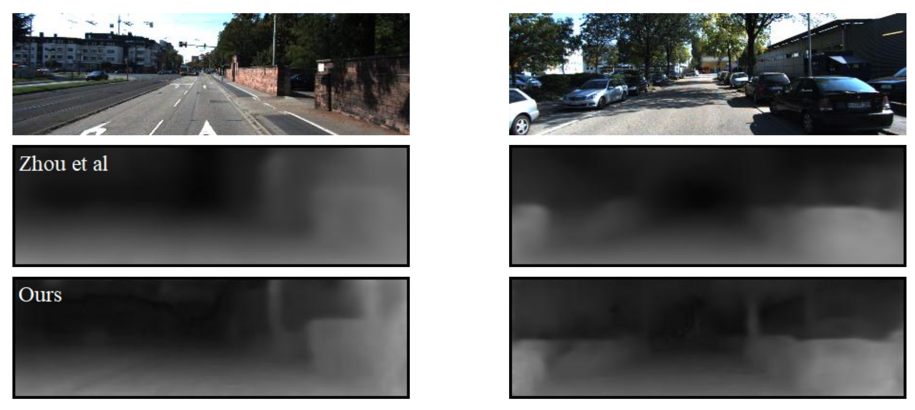
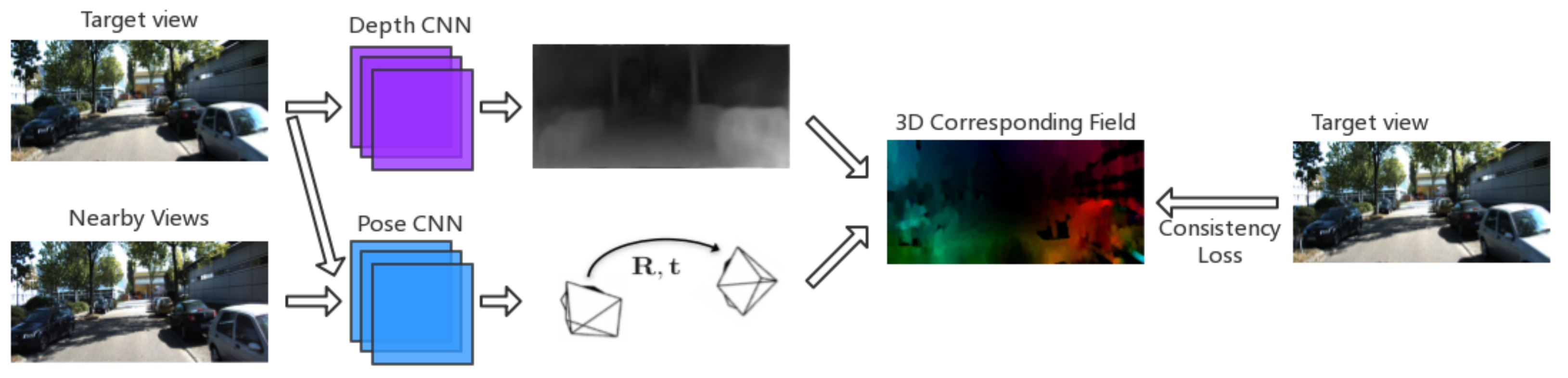
In this paper, we propose a deep prediction method based on unsupervised learning. This method trains the neural network by analyzing the geometric constraint relationship of the three-dimensional (3D) scene among sequence of pictures and constraining the correspondence of pixels among images according to image gradient. It can simultaneously predict the depth structure of the scene and the ego-motion. Our method is introducing a loss which penalizes inconsistencies in 3D pixel corresponding field and 2D images. Different from the existing method based on pixel corresponding in 3D-3D alignment like [
14,
15], we introduce a 3D-2D method which also proved effective. We first project the pixel points in the image into the 3D space and then calculate the 3D corresponding vector field of the pixels according to the ego-motion and the depth map predicted by the neural network. The 3D corresponding vector field is smoothed based on the 2D image by minimizing the smoothing loss of the vector filed according to the pixel gradient. The smoothing of the 3D corresponding vector field makes the gradient of 3D corresponding consistent with the gradient of 2D image, which effectively improves the details in the prediction result. Example predictions are shown in
Figure 1.
The main contributions of this paper are:
We propose a depth prediction method for AMP based on unsupervised learning, which can learn from video sequences and simultaneously estimate the depth structure of the scene and the ego-motion.
Our method makes the spatial correspondence between pixel points consistent with the image area by smoothing the 3D corresponding vector field by 2D image. This effectively improves the depth prediction ability of the neural network.
The model is trained and evaluated on the KITTI dataset provided by [
16]. The results of the assessment indicate that our unsupervised method is superior to existing methods of the same type and has better quality than other self-supervised and supervised methods in recent years.
2. Related Work
Traditional Monocular Methods: Traditional monocular methods always use multi-view information to estimate depth of scene. Structure from motion (SfM) and simultaneous localization and mapping (SLAM) are typical ones of traditional methods. Since the depth of the object in the image cannot be directly calculated, the SLAM methods based on monocular camera need to first analyze the relationship of the position of the same points in different views, and then estimate the ego-motion and the depth of the points in the scene simultaneously for example [
6,
7]. Therefore, points in different views first need to be matched with each other.
In general, there are two ways to match pixels points in different views: indirect matching methods and direct matching methods [
7,
17]. Indirect matching, which is also known as keypoint-based methods, first extract feature points in images and calculate feature descriptors, and then match points in different views according to their descriptors [
6] are typical indirect matching method. This type of method only matches hundreds of feature points in entire image, only the depth of the feature points can be estimated, dense depth information cannot be reconstructed. In contrast, direct matching, which is also known as dense-based methods, can provide dense depth map of the whole image. Refs. [
18,
19] are typical direct matching method. Dense-based methods first smooth the images, and then project points in source image to target image and calculate reprojection error, finally camera position and scene depth are optimized by minimizing the reprojection error. This inspired people to use geometric constraints for the training of neural networks. Dense-based method minimizes the reprojection error to optimize depth map and ego-motion, while learning-based method minimizes the reprojection error to optimize weight factor of neural networks.
CNN for Geometry Understanding: A typical CNN structure consists of convolutional layers and fully connected layers, and this structure is widely used in the fields of image recognition and target detection, for example [
4], etc. [
20] applied a typical CNN structure in depth prediction. However, due to the existence of fully connected layers, the 2D feature map obtained through the convolutional layers needs to be converted into a 1D feature vector of a specific length before being passed into fully connected layers. In this step the spatial relationship between the image pixels is lost and the size of the input image is limited. The fully connected layer is not suitable for dense-to-dense predictions, so fully convolutional network containing only convolutional layers and pooling layers emerges and gets applied to image segmentation in [
21]. Ref. [
12] improved their prior work with fully convolutional network. Ref. [
22] extended the traditional deep neural network by adding a residual structure to the network, which effectively improved the training efficiency. Ref. [
23] applied this residual neural network to the depth estimation of the scene.
On the basis of [
20,
24] combined with conditional random fields (CRFs) to jointly estimate depth and semantic segmentation information from a single image. Ref. [
25] constructed a joint optimization depth network to realize the joint estimation of semantic segmentation and depth calculation [
26] regarded the single image depth estimation problem as a multi class classification problem, and estimated the corresponding depth value of each pixel by training the depth neural network classifier. Ref. [
27] adopted fully convolutional network and optical flow as auxiliary information to achieve depth estimation of the occluded areas in the image.Liu et al. [
28] skillfully combined continuous conditional random field (CRF) with deep convolutional neural networks (DCNNs), and proposed a deep convolutional neural field to estimate depth from a single image, particularly, the method proposed by [
28] applied to general scenes without any prior and extra information. Ref. [
29] proposed a multi-scale depth estimation method, extract depth information and gradient information using a dual flow network and then fused to perform depth estimation.
At the same time, researchers have also explored the ability of deep learning methods to estimate the ego-motion among views. Ref. [
30] proposed a method for estimating ego-motion from video images by training neural networks through LIDAR data. In their method, the LIDAR provides the depth information of the scene, thus the ego-motion can be easily guaranteed, but the LIDAR data are not easy to obtain compared to the image data. By combining the CNN network and the RNN network, Ref. [
31] fused video sequence and inertial sensor (IMU) data to estimate the ego-motion. However, their work did not consider depth information of the scene.
Unsupervised Learning of Depth Estimation: The depth estimation methods based on unsupervised learning share the same kernel with the dense SLAM method, that is projecting images of different views, and calculating reprojection error as the loss function. The difference from the dense SLAM method is that the unsupervised learning methods minimize the reprojection error to optimize the parameters of the neural network, which enables the neural network to output the correct depth information.
Calculating reprojection error requires the depth structure of the scene and ego-motion. Ref. [
4] proposed an auto-encoder network based on the binocular vision for depth estimation. This method predicts the depth structure from the image of a single camera and projects it to another camera to calculate the reprojection error. The binocular vision-based approach depends on the accuracy of the ego-motion. However, the binocular vision system requires complex configuration and calibration. Ref. [
5] proposed a complete unsupervised depth estimation method, which predicts the depth of a single image and the ego-motion among views and calculates the reprojection error by warping nearby views to the target using the predicted depth and ego-motion, which make it possible to train the network using monocular video sequence.
Ref. [
15] used stereo images as training supervision, and synthesized images by introducing left and right parallax consistency and estimating stereo parallax based on deep network;then the neural network is trained to estimate the depth of a single image by comparing the grayscale difference between the input stereo image and the composite image. Ref. [
32] estimated the depth information in a single image by using two CNN modules on the basis of [
15]. Ref. [
33] extended the method in [
15], using monocular image sequence or binocular stereo image sequence as training data and composite image as supervision data to achieve depth estimation. Rezende et al. [
34,
35] used encoder-decoder architecture of 3D CNN to achieve 3D reconstruction of single image, the former infers the three-dimensional model of the scene directly from the two-dimensional image in the way of probability reasoning, and uses the three-dimensional model as the supervision to train; the latter, according to the given perspective, renders the corresponding projected images from the 3D model generated by the deep network as additional supervision to train the network. Ref. [
36] used monocular image sequences as training data and predicted depth, posture, semantic segmentation and other information according to the depth estimation neural network module, attitude estimation neural network module and image segmentation neural network module. Ref. [
37] proposed GeoNet, a network framework used to learn monocular depth, video motion estimation and optical flow information, which effectively solved the problems of image occlusion and texture blurring. Ref. [
38] presented the first learning based approach for estimating depth from dual-pixel cues. In order to solve the limitation of monocular depth estimation algorithm due to the lack of high-quality datasets, Ref. [
38] captured a large dataset of in-the-wild five-viewpoint RGB images paired with corresponding dual-pixel data.
Because of the similarity between the unsupervised learning methods and the dense SLAM methods, problems in the dense SLAM methods are also reflected in the unsupervised deep learning methods. Due to geometric constraints, the monocular SLAM methods cannot estimate the real scale of the scene. In unsupervised learning methods, a smaller inverse depth scale always results in smaller loss value, which makes predicted depth continue to shrink as the training process approaches until it approaches zero and hinders the converge of the training result process. Ref. [
39] effectively suppressed the reduction of the output by normalizing the inverse depth of the output. However, their methods still have poor performance in thin structure and the detail quality of the depth map. In this paper, we improve the typical unsupervised method by involving a loss function based on pixel corresponding consistency, which makes our networks recover more detail of depth information and improves the depth estimation results in thin structure regions.
4. Experiments and Discussion
In this section, we first introduce the network structure of our model, and its training details of it. Then we introduce the datasets and compare the performance of our method with other similar methods.
4.1. Network Structure
There were two sub-nets in our framework: the depth estimation network and the ego-motion estimation network. The depth estimation network predicated one-channel depth map of four different scales from a single three-channel image while the ego-motion estimation network predicated six-DOF of ego-motion from three consecutive images.
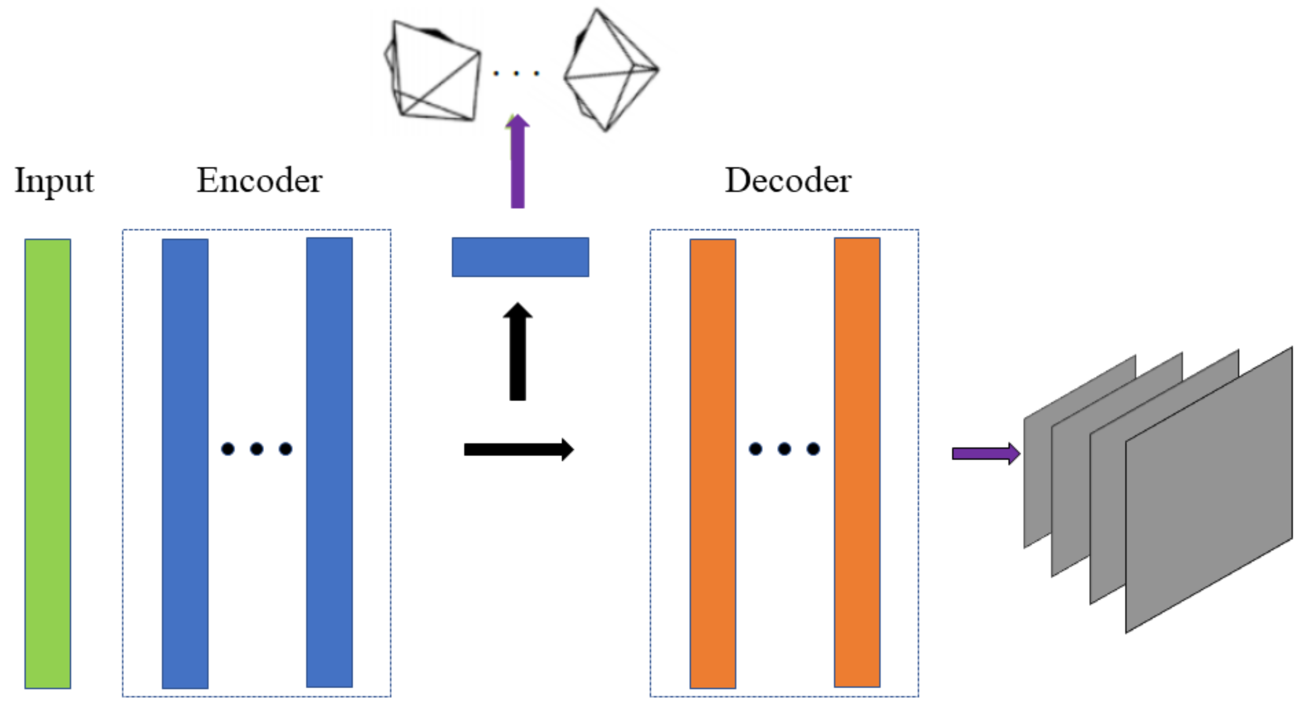
The depth estimation network was based on the [
44] network structure, that is also adopted by [
5]. As show in
Figure 4, this network structure could be divided into encoder part and decoder part, adding a skip structure and adopting an output of four scales. The overall network structure is shown in
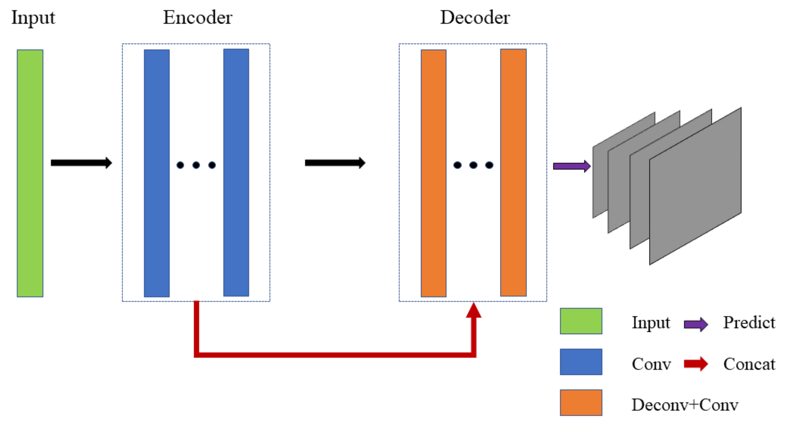
Table 1. Since the full convolutional neural network did not restrict the size of the input image, the two columns of the table, input size and output size, indicate the ratio of the image edge length to the original image. Except for the predicted output layer, each convolutional layer was activated by the RELU activation function. Since the inverse depth result of the output was not conducive to network calculation, we multiplied the output by 10 to control it within the appropriate range and added 0.01 to prevent the error caused by little values.
The encoder included 14 layers, all of which were convolutional layers. The output size of every two layers was the same, divided into a group. The input of the first group (conv1a and conv1b) was the original image, the size of the convolution kernel was 7 × 7, and the output size was a feature map of 1/2 of the original image. Each subsequent group was similar to the first group, and the output size of the previous group was 1/2 of the input feature map.The dimension of the feature graph increased with the depth of the network and finally reached 512.
The decoder was complex, including convolutional layer and deconvolutional layer. Like the encoder, the decoder was divided into a group with the same output size every two layers. The first group consisted of upconv7 and icnv7 layers. upconv7 was the reverse convolution layer. Unlike convolution layer, the deconvolution layer enlarged the feature map and output the result with the output size of twice the input. icnv7 was the convolutional layer, and the input contained skip structure, i.e., the upconv7 was superimposed with the conv6b in the encoder as the input, thus preserving the detailed features of the shallow layers. The second group (upconv6 and icnv6) and the third group (upconv5 and icnv5) were similar in structure to the first group. After one group, the feature map size was doubled. The fourth group was different from the first three groups by adding the output layer pred4, which output the estimation result of one dimension. The overall structure of the fifth group was similar to that of the fourth group, while the skip structure was more complicated. The skip structure of the convolutional layer icnv3 superimposed upconv3 and conv2b, and at the same time enlarged the output result of pred4 to pred4up and superimposed it, while ensuring that the deep global information and the shallow detail information were preserved. The sixth group (upconv2, icnv2 and pred2) had the same structure as the fifth group. In the seventh group (upconv1, icnv1 and pred1) structure, because there was no feature layer with the same size as the original image, the skip structure of the convolution layer iconv1 superimposed upconv1 with the result pred2up of the previous layer’s estimation.
The depth estimation network structure did not include a fully connected layer and a pooling layer. The disadvantage of the fully connected layer was that the fixed feature vector length limited the input size, and the transformation of the feature vector lost the spatial characteristics of the pixel. In traditional convolutional neural networks, the pooling layer is used for downsampling, so information loss will occur. The direct use of a convolutional layer with a step size of 2 to achieve downsampling circumvented this problem.
The ego-motion estimation network had the same network structure used in [
5]. As show in
Figure 5. The network input several continuous images in the image sequence, output six-DOF camera motion, and output masks of four scales corresponding to the depth map, which were used to exclude the non-rigid body parts in the scene. In the ego-motion vector, the position change part was divided by the average of depth, so that the motion of the camera corresponded to the scale of the depth map.
The camera motion estimation part of the network was dense to sparse estimation, so the deconvolution layer was not adopted and only contained three convolution layers. The structure is shown in
Table 3, where
N is the number of target images in the image sequence. The mask estimation part of the network was dense to dense estimation, which contained only five deconvolution layers and four output layers. The structure is shown in
Table 4, where
N is the number of target images in the image sequence.
4.2. Datasets Description
In the experiments, three widely used depth estimation datasets were used to test the proposed approach: KITTI, Apolloscape [
45] and Cityscapes [
46].
KITTI dataset was the largest data set for evaluating computer vision algorithms in autonomous driving scenarios in the world. It collected 61 scenes including rural areas and urban highways with optical lenses, cameras, LIDAR and other hardware equipment. There were at most 30 pedestrians and 15 cars in the image, and there were different degrees of occlusion. The normal RGB image resolution in KITTI was 375 × 1242 and the ground-truth depth resolution was 228 × 912. The original KITTI dataset did not have a true depth map, but contained sparse 3D laser measurements captured with the Velodyne laser sensor. To be able to evaluate in the KITTI dataset, we needed to map the laser measurements into the graph space to generate the ground-truth depth corresponding to the original image.
The Cityscapes dataset, jointly provided by three German companies, including Daimler, contains stereo vision data for more than 50 cities, with higher resolution and quality images. It contained a rich and distinct set of scenes from KITTI. Compared to the KITTI dataset, the images from the Cityscapes dataset were of better quality, with more diverse shooting scenes and higher resolution.
Apolloscape dataset was provided by the company, including perception, the simulation scene, road network data, such as hundreds of frames per-pixel semantic segmentation of high-resolution image data, as well as the corresponding per-pixel semantic annotation, dense point cloud, three-dimensional images, three-dimensional panoramic images, and further more complex environment, weather and traffic conditions, etc.
4.3. Experiment Settings
In this paper, the KITTI2012 dataset [
16] was used to train the neural network. In the training, the resolution of the image was set to
. Since the network structure is full convolutional, the image of any size can be used in the actual test. In this paper, TensorFlow [
42] was used to build a neural network, and the Adam [
43] optimizer was used. The learning rate was set to 0.001, and the training process usually converged after about 150 K iterations.
For the evaluation of depth results, this paper used the same indicators and test set partitioning as [
12]. This division included 700 images from the KITTI test dataset (this division excludes visually similar images). During the assessment, the effective distances were set to 50 m and 80 m, respectively, and each method was evaluated using the error used in [
12].
The evaluation criteria included Absolute Relative error (Abs Rel), Square Relative error (Sq Rel), Root Mean Squared Error (RMSE) and Root Mean Squared logarithmic Error (RMSE log). For the absolute relative error and square relative error, this paper adopted the calculation method in [
20]. For RMSE, it could be calculated by the following formula:
where,
n is the total number of pixels, and
and
are the actual and estimated depths, respectively. RMSE log could be calculated according to the following formula:
The parameters were the same as Formula (
12).
For camera position estimation, two sequences Seq.09 and Seq.10 in KITTI dataset were used in this paper. The evaluation index was Absolute Trajectory Error (ATE), which could be calculated according to the following formula:
where
is the actual pose of the camera,
is the estimated camera pose, and
is the similar transformation matrix from the estimated pose to the actual pose.
4.4. Comparisons with Other Methods
To demonstrate the superiority of our method, we compared it with some classical methods, including supervised methods [
13,
20] and unsupervised methods [
4,
5]. The ground-truth depth was from LIDAR data, which were obtained by projecting the point cloud to the image plane.
4.4.1. Evaluation of Depth Estimation
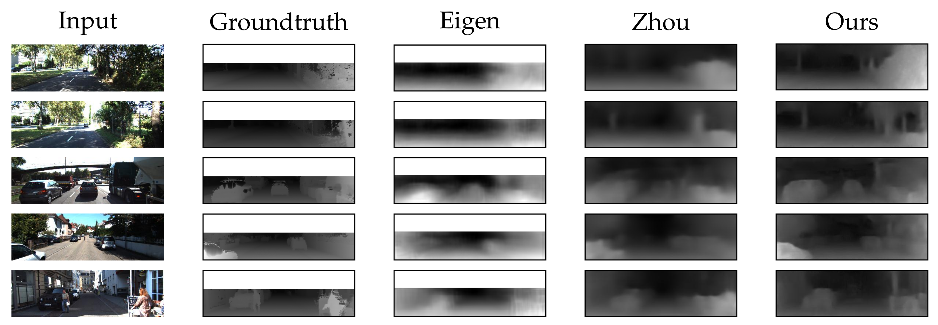
Table 5 compares the results of our work with existing work in estimating the depth of the scene. As seen in
Table 5, “Ours” and “Ours consis” indicate the results of using and not using the consistency constraints, respectively. Experimental results showed that our method was significantly better than supervised learning methods, which showed that our method overcame the impact of the supervised learning method on the results due to the poor quality of the supervised data. Compared with the benchmark work [
5], our results reduced the average error from 0.208 to 0.169, which reflected the effectiveness of our method. Our results still had some gaps with the results of the stat-of-the-art method of 0.148 by Godard [
15] since their method used images with known camera baseline as supervised data, we believe that the gap is due to our method not further constraining the ego-motion. In addition, the consistency loss further narrowed the error from 0.176 to 0.169, which reflected the effect of our loss term.
Figure 6 is a qualitative comparison of visualizations. The experimental results reflected the ability of our method to understand 3D scenes, that is, the method successfully analyzed the 3D consistency of different scenes.
4.4.2. Evaluation of Ego-Motion
During the training, the result of motion estimation greatly affected the accuracy of depth estimation. In order to evaluate the accuracy of our method in camera motion estimation, we conducted an experiment on the KITTI odometry split dataset. This data set contained 11 video sequences and their corresponding sensor information which are obtained through IMU/GPS. We used the sequence 00–08 to train the model, and the sequence 09–10 to evaluate it. Additionally, we compared our method with a typical visual odometry of ORB-SLAM [
6]. ORB-SLAM is an indirect SLAM method which calculates camera motion and scene depth through feature point matching. It has a bundle adjustment back-end based on graph optimization, which further constrains ego-motion by non-adjacent images. Therefore, we compared our approach to two different SLAM processes: (1) “ORB-SLAM (short)” containing only five frames as input, which had no graph optimization; (2) “ORB-SLAM (full)” containing the entire process and all frames. As shown in
Table 6, we compared our method with existing work on ego-motion estimation. Our method outperformed other unsupervised learning methods, approaching the ORB-SLAM with global optimization.
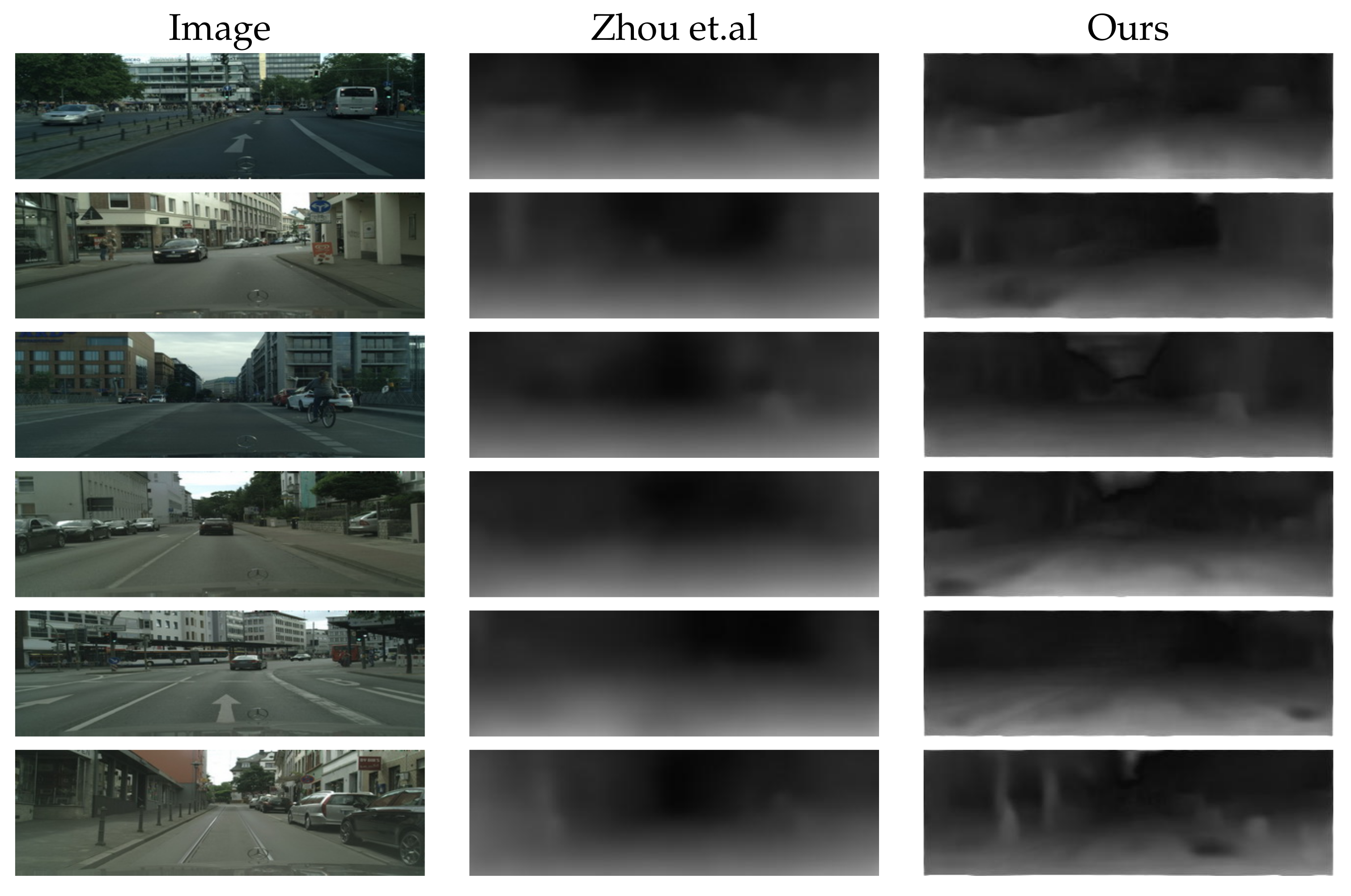
4.4.3. Depth Results on Apollo and Cityscapes
To prove the versatility of our method, we directly applied our model trained on KITTI to the Apollo stereo test set [
45] and Cityscapes test set. Our model could still output accurate prediction results, even if the scene structure was more complex. As shown in
Figure 7 and
Figure 8, our method could recover more details.


