A Noise Robust Micro-Range Estimation Method for Precession Cone-Shaped Targets

Abstract

The estimation of micro-Range (m-R) is important for micro-motion feature extraction and imaging, which provides significant supports for the classification of a precession cone-shaped target. Under low signal-to-noise ratio (SNR) circumstances, the modified Kalman filter (MKF) will obtain broken segments rather than complete m-R tracks due to missing trajectories, and the performance of the MKF is restricted by unknown noise covariance. To solve these problems, a noise-robust m-R estimation method, which combines the adaptive Kalman filter (AKF) and the random sample consensus (RANSAC) algorithm, is proposed in this paper. The AKF, where the noise covariance is not required for the estimation of the state vector, is applied to associate m-R trajectories for higher estimation accuracy and lower wrong association probability. Due to missing trajectories, several associated segments which are parts of the m-R tracks can be obtained by the AKF. Then, the RANSAC algorithm is utilized to associate the segments and the complete m-R tracks can be obtained. Compared with the MKF, the proposed method can obtain complete m-R tracks instead of several segments, and avoids the influence of unknown noise covariance under low SNR circumstances. Experimental results based on electromagnetic simulation data demonstrate that the proposed method is more precise and robust compared with traditional methods.

1. Introduction

With increasing human activities in outer space, research of space targets has attracted more and more attention [1,2]. Usually, a target, or any structure on a target, undergoes micro-motion dynamics in addition to bulk motion. Precession is one of the typical micro-motions for space targets, such as cone-shaped targets [3,4,5,6]. The precession dynamic induces modulations on echoes, from which micro-Range (m-R) can be obtained [7,8]. By estimating and analyzing scattering centers’ m-R, high-resolution radar imaging, together with the motion and structure parameters, can be precisely acquired [5].

A scattering model of the precession cone-shaped target is proposed in [9,10,11]. There are three scattering centers on the model, one is located on the smooth apex of the cone and the other two are located at the intersection of the circular edge and the bottom plane, respectively. There are some weak scattering centers on the cone-shaped target whose scattering power is lower or close to noise power. Therefore, the sidelobes of dominant scattering centers and high noise interference make it difficult for m-R estimation of weak scattering centers in a low signal-to-noise ratio (SNR) condition.

Recently, many methods have been proposed to estimate m-R from wideband radar echoes. These methods can be divided into two categories: image domain methods and signal domain methods. In image domain methods, m-R curves can be extracted from the range–time image [12,13,14]. In [13], the generalized Radon transform with the CLEAN technique (GRT-CLEAN) is proposed to obtain each m-R curve, respectively, by searching for the peak of the parameter domain spectrogram. In the parameter domain spectrogram, the sinusoidal curve in range–time can be mapped to a point in the parameter domain by the generalized Radon transform (GRT) [12,13], and the CLEAN technique [15] is applied to reduce the effect of unavoidable sidelobes in the range–time image. The radon transform can accomplish the connection of broken segments and the selection of overlapped segments. However, this method bears a heavy computational burden for constructing a multidimensional parameter domain spectrogram. A improved genetic algorithm with the CLEAN technique (GA-CLEAN) is proposed in [14], which converts the complex imaging problem to a parametric optimization problem. Compared with the GRT-CLEAN method, this algorithm is not required to construct the spectrogram, and has a good convergence property. However, the limited range resolution of the range–time image limits the estimation accuracy of image domain methods.

Signal domain methods can obtain a super-resolution range estimation to improve estimation accuracy. There are two types of signal domain method. The first type of method obtains a super-resolution m-R estimation result by analyzing signal subspace [16,17,18]. In [18], estimation of signal parameters via rotational invariance techniques (ESPRIT), which exploits the rotational invariance of the underlying signal subspace, is applied to estimate m-R. However, this method is ineffective since it obtains the wrong signal subspace under high noise interference. In the second type of signal domain, trajectories of scattering centers are extracted by the sparse signal representation algorithm, and then the trajectory association algorithm is applied to associate the trajectories. In [19], the Kalman filter is applied to associate trajectories. However, the Kalman filter suffers from the intersecting trajectory and spurious trajectory problems. In [20], a modified Kalman filter (MKF) is proposed to associate the intersecting trajectories for instantaneous frequency estimation. In the MKF, the Kalman filter is used to associate the trajectories and the trajectory correction strategy is applied to correct wrong association. However, since trajectories of the weak scatter center cannot be extracted under low SNR circumstances, several associated segments, not the complete m-R tracks, will be obtained by the MKF. In addition, the MKF, where the process covariance initialized without any prior knowledge, is usually inaccurate or mismatched, provides poor performance in robustness, and results in wrong associations, especially under low SNR circumstances. Substantial association corrections will increase the cost time.

In this paper, a trajectory association method, which combines the adaptive Kalman filter (AKF) [21] and the random sample consensus (RANSAC) algorithm [22], is proposed to obtain complete m-R tracks and deal with the unknown noise covariance problem in a low SNR circumstance. In the proposed method, the AKF, which avoids the influence of the unknown covariance matrix of process noise, is applied to associate m-R trajectories. The AKF estimates the state vector by prior error covariance, which is directly reconstructed through online excavating of the posterior prior error covariance sequence, instead of needing the covariance matrix of process noise. Due to the missing trajectories, several associated segments which are parts of the m-R tracks can be obtained. Then, the RANSAC algorithm is utilized to associate the segments by estimating the parameters of each m-R track model. The RANSAC algorithm finds the parametric model for each m-R track, which contains maximum inlier trajectories, from many hypothetic parametric models, and the complete m-R tracks can finally be obtained.

There are many variants of the RANSAC algorithm. In [23], a good sample consensus (GOODSAC), which replaces random sampling with an assessment driven selection of good samples, can foster precision and proper utilization of computational resources. However, a GOODSAC relies on the priori mathematical or geometric model to produce a list of good samples. In this paper, since there is no priori information of the mathematical or geometric model, a GOODSAC is not applicable for the connection step. In [24], a locally optimized RANSAC improves the performance by choosing better samples. In this paper, all trajectories in one segment are used to form a sample set, and we perform a complete search to test all sample sets formed by all segments to ensure precise estimation results. Therefore, samples do not need to be chosen, and the locally optimized RANSAC is not applicable for the connection step. Maximum Likelihood SAC (MLESAC) utilizes probability distribution of error by inlier and outlier to evaluate a hypothesis [25]. It adopts the same sampling strategy as RANSAC to generate putative solutions, but chooses the solution that maximizes the likelihood of inliers and outlier rather than the number of inliers. In this paper, since almost all the outliers have been filtered out in the associated step, MLESAC should provide almost the same results, with more computation burden compared to the RANSAC algorithm. We will offer a more detailed analysis with the comparative experiment in Section 4. In [26], the Randomized RANSAC (R-RANSAC) performs a preliminary test to reduce time. Hypothesis evaluation is only performed when the generated hypothesis passes the preliminary test. However, a valid hypothesis may be mistakenly rejected by the preliminary test [27]. In summary, to obtain precise and robust results, the RANSAC algorithm is chosen to associate the segments.

Compared with the MKF, the proposed method can obtain complete m-R tracks instead of segments, and has a better performance on the estimation accuracy and time cost. Firstly, by estimating the parameters of the m-R track model in the proposed method, the complete m-R tracks rather than segments can be obtained, which overcome the shortcoming of the MKF. Secondly, when noise covariance is inaccurate or mismatched, the proposed method can obtain higher accuracy estimation results and decrease wrong association probability under low SNR circumstances. Since the covariance matrix of process noise is not required for the calculation of prior error covariance, the performance of AKF is not affected by the unknown covariance matrix of process noise. Finally, since it decreases wrong associations and association corrections, the AKF can significantly reduce time cost. Compared with ESPRIT, the proposed method has better noise robustness. Compared with image domain methods, the proposed method can obtain a super-resolution range estimation to improve estimation accuracy. Experimental results on electromagnetic simulation data demonstrate that the proposed method is more accurate and more time-saving compared with the methods introduced above.

The organization of this paper is as follows. The signal model and trajectory extraction method are provided in Section 2. The proposed association method is developed in Section 3. The detailed experimental results, based on electromagnetic simulation data, are given in Section 4. Section 5 concludes this paper.

2. Signal Model and Trajectory Extraction

2.1. Geometric Model and Signal Model

In this section, the geometric model and the signal model of the precession cone-shaped target are introduced. Figure 1 shows the model in the coordinate system $O-XYZ$, where the precession center of the target is located at the origin $O$. The target spins around the target symmetry axis at an angular velocity $w_s$, and rotates around the axis ${\mathsf{\Omega }}_N$ at an angular velocity $w_c$, which forms the precession motion. For simplicity, ${\mathsf{\Omega }}_N$ and the radar line-of-sight (rLOS) are on the $YOZ$ plane, and the symmetry is located at the Z-axis initially. The precession angle between the coning axis and the symmetric axis is $\alpha$, and the initial target line-of-sight angle between the symmetric axis and the rLOS is $\beta$. The distance between the precession center and the radar is $R_0$.

In this scattering center model, the target contains three main scattering centers, where the scattering center $P_2$ and $P_3$ are located at the intersection of the circular edge, and the bottom plane and $P_1$ is located on the smooth apex of the cone. The initial coordinate of the scattering center $P_1$ is $p_{10}=(0,0,H)$ and the initial coordinates of the scattering center $P_2$ and $P_3$ are $p_{20}=(0,r_a,-h)$ and $p_{30}=(0,-r_a,-h)$, where $H$ denotes the distance between the precession center and the apex of the cone, $h$ is the distance between the precession center and the bottom plane, and $r_a$ is the radius of the bottom plane. In this paper, we ignore the influence of bulk motion. According to [5], the range between scattering centers and radar can be obtained by

$$\{\begin{array}{l}{r}_1(t)=R_0-(H-h)\cos \gamma (t)\\ r_2(t)=R_0+h\cos \gamma (t)+r_a\sin \gamma (t)\\ r_3(t)=R_0+h\cos \gamma (t)-r_a\sin \gamma (t)\\ \cos \gamma (t)=\cos \alpha \cos (\alpha +\beta )-\sin \alpha \sin (\alpha +\beta )\cos (w_{c}t)\end{array}$$

(1)

where $\gamma (t)$ denotes the angle between the rLOS and the symmetric axis at $t$ time step. The micro-Range curve of $P_1$ is sinusoidal and the micro-Range curves of $P_2$ and $P_3$ can be described as sinusoidal curves, approximately [4].

Here, the transmitted signal $s_t(t)$ is the linear frequency modulated signal

$$s_t(t)=rect\left(\frac{t}{T_p}\right)\exp (j2\pi f_{c}t+j\pi \mu t^2)$$

(2)

where $rect(t/T_p)$ denotes a rectangular pulse of the pulse width $T_P$, $f_c$ denotes the radar center frequency, and $\mu$ denotes the linear frequency modulated coefficient with the bandwidth $B=\mu T_p$. According to [28], the high-frequency scattering responses of a target can be described as a sum of responses from individual scattering centers, approximately. The echoes of the space target in a pulse are denoted as

$$s_r(t)={\displaystyle \sum _{i=1}^I{a}_i}rect(\frac{t-R_i}{T_p})\exp (j2\pi f_c(t-R_i)+j\pi u{(t-R_i)}^2)$$

(3)

where $I$ is the number of scattering centers on the target, $R_i$ denotes the distance between the $i$th scattering center and the radar which is assumed to be constant in a pulse, $a_i$ is the corresponding scattering coefficient of the $i$th scattering center, and $c$ denotes the wave propagation velocity.

To obtain the range profile, the “dechirp” processing technique [29] is applied to obtain

$$\begin{array}{l}{s}_{if}(t)=s_r(t)\cdot s_{ref}(t)\\ ={\displaystyle \sum _{i=1}^I{a}_{i}rect\left(\frac{t-2R_i/c}{T_p}\right)\exp \left(-j\frac{4\pi u}{c}\left(t-\frac{2R_{ref}}{c}\right)R_{\Delta }-j\frac{4\pi }{c}{f}_c{R}_{\Delta }+j\frac{4\pi u}{c^2}{R}_{\Delta }^2\right)}\end{array}$$

(4)

where the reference signal $s_{ref}(t)$ can be written as

$$s_{ref}(t)=rect(\frac{t-2R_{ref}/c}{T_{ref}})\cdot \exp (j2\pi f_c(t-\frac{2R_{ref}}{c})+j\pi u{(\widehat{t}-\frac{2R_{ref}}{c})}^2)$$

(5)

In the reference signal, the relative range $R_{\Delta }=R_i-R_{ref}$, $R_{ref}$ denotes reference range, $T_{ref}$ denotes the reference pulse width, which is a little greater than $T_p$. Usually, $\frac{u}{c^2}{R}_{\Delta }^2<<\frac{f_c{R}_{\Delta }}{c}$. Then, Equation (5) can be written as

$$s_{if}(\tilde{t})={\displaystyle \sum _{i=1}^I{a}_{i}rect\left(\frac{\tilde{t}-2R_{\Delta }/c}{T_p}\right)\exp \left(-j4\pi \frac{R_{\Delta }}{c}\left(u\tilde{t}+f_c\right)\right)}$$

(6)

where $\tilde{t}=t-\frac{2R_{ref}}{c}$, $t\in \left(0,T_p\right]$. We proceed $P$ times down-sampling in time $\tilde{t}$ where the sampling interval is $△t=\frac{T_p}{P}$. Then, the discrete frequency echoes can be expressed by

$$s_{if}(p)={\displaystyle \sum _{i=1}^I{a}_i\exp (-j\frac{4\pi R_{\Delta }}{c}{f}_p)}$$

(7)

where $f_p=f_c+p\frac{B}{P}$. Let $r_n=n\Delta r,n=1,2,\dots ,N$ where $N\Delta r$ denotes the scene swath. Then, the over-complete basis is constructed as follows:

$$X[n,p]=\exp (-j4\pi r_n{f}_p/c)$$

(8)

Taking into account the noise, the echoes can be rewritten as

$$S_{1\times P}=A_{1\times N}{X}_{N\times P}+noise$$

(9)

where $A=\left[0,0,\dots ,a_i,\dots 0\right]$ denotes the sparse coefficient vector of the echoes. Obviously $A[n]=a_i$ when $R_i-R_{ref}=R_{\Delta }=n\Delta r$. The interval $\Delta r$ determines the range extraction precision which should be sufficiently small for constructing the over-complete dictionary and the super-resolution range estimation.

2.2. Trajectory Extraction via the Sparse Signal Representation Algorithm

In this section, the orthogonal matching pursuit (OMP) algorithm, which is a kind of sparse signal representation algorithm, is applied to obtain the m-R trajectories. According to the signal model of the space coning-shaped target introduced above, $A$ denotes the scattering coefficients from the target scattering centers, and the indexes of non-zero elements denote the ranges between scattering centers and radar. $A$, which is a sparse vector, can be estimated by solving the following sparse optimization problem

$$\widehat{A}=\arg \underset{A}{\min }{\Vert A\Vert }_0\mathrm{s}.\mathrm{t}.{\Vert S-AX\Vert }_2<\delta$$

(10)

where ${\Vert ·\Vert }_2$ denotes the $l_2$ norm, ${\Vert ·\Vert }_0$ denotes the $l_0$ norm, and $\delta$ denotes the noise power, which can be regarded as the heat noise from the receiver and accurately obtained by estimating the power of the non-target region in the HRRPs [30,31].

Solving Equation (10) is an NP-hard problem. The OMP algorithm can be used for (10) to attain the approximate solution. OMP is an iterative greedy algorithm. In this algorithm, the column of $X$, which is most strongly correlated with the residual, is chosen, and the corresponding element in $\widehat{A}$ can be calculated in the meantime. Then, the residual is updated by subtracting the contribution of this signal component at each iteration until residual power is lower than noise power $\delta$. The estimated coefficient vector $\widehat{A}$ can be obtained at last where the non-zero elements are the scattering coefficients and the indexes of non-zero elements correspond to the range cells of scattering centers. The range of scattering centers can be regarded as the extracted scattering center trajectories. The extracted scattering center trajectories are shown in Figure 2.

In the low SNR condition, the power of echoes of the weak scattering center is close to noise power, and the inevitable estimation error makes the estimated noise power $\delta$ larger than that of the weak scattering center. Therefore, it may be impossible to extract the weak scattering centers and a large number of spurious trajectories are extracted undesirably. Besides, near the intersection of m-R curves, the multiple signal components are not separated for the limitation of resolution in the OMP algorithm. Hence, the range estimation of scattering centers is inaccurate and the scattering centers may be missing near the intersection.

3. Trajectory Association by Adaptive Kalman Filter

In this section, we propose an algorithm combining the AKF and the RANSAC algorithm for associating the trajectories. The associated method can associate the trajectory of the same scattering center, and the associated method can also filter out spurious trajectories extracted from the noise component. After that, the track of the scattering center, which is regarded as the m-R curve of the scattering center, can be obtained. In [20], a trajectory association method based on the MKF is proposed to estimate the instantaneous frequency. In MKF, the Kalman filter is applied to associate trajectories, and the trajectory correction strategy is applied to correct wrong associations. For the association of m-R trajectories, the missing trajectories of weak scattering centers will make the track broken. In addition, the process noise matrix, which is initialed without any prior knowledge, is usually inaccurate, or even mismatched. To solve these problems, the AKF, which does not rely on prior and correct knowledge about the dynamical model, is applied to associate the trajectories, and the broken segments are processed to obtain the complete m-R track. The details of the proposed method are given in the following.

Due to precession dynamics, the m-R tracks are modulated as sinusoidal. Therefore, to describe the trajectory association problem, the discrete system with the linear Gaussian dynamic and measurement model is proposed, which satisfies the following equation:

$$\{\begin{array}{l}{X}_{k+1}^i=F{X}_k^i+n_k^i,n_k^i\sim N(0,R_n)\\ Y_k^i=diag({\chi }_k^i)*(C{X}_k^i)+(E-diag({\chi }_k^i))v_k^i,v_k^i\sim N(0,R_v)\end{array}$$

(11)

where $X_k^i$ is the state vector of $i$th scattering center at time step $k$, $n_k^i$ is the process noise, which is a zero-mean Gaussian random process with the covariance $R_n$, and $F$ is the state transition matrix. Additionally, the measurement $Y_k^i$ originates from $i$th scattering center at time step $k$, where ${\chi }_k^i\in \left\{0,1\right\}$ indicates whether the $i$th scattering center is measured at time step $k$. ${\chi }_k^i=0$ indicates the scattering center is missing and the measurement is regarded as the random noise trajectory. $v_k^i$ denotes the measurement noise, which is a zero-mean Gaussian random process with the covariance $R_v$. $E$ is the identity matrix and $C$ is the measurement matrix. The process noise $n_k^i$ and the measurement noise $v_k^i$ are statistically independent.

In the range–time domain, the instantaneous m-R track can be described as a smooth scattering center track, and the constant velocity (CV) model is adapted to describe its shape. In the CV model, the state vector is $X_k^i={[x_k^i,{\dot{x}}_k^i]}^T$, where $x_k^i$ denotes the range and ${\dot{x}}_k^i=\frac{x_k^i-x_{k-1}^i}{\Delta t}$ denotes the velocity, and the velocity is approximately constant in a short time. $\Delta t$ denotes the time between two contiguous time steps. The state transition matrix $F=\left[\begin{array}{cc}1& 0\\ 1& 1\end{array}\right]$ and the measurement matrix $C=\left[\begin{array}{cc}1& 0\\ 0& 0\end{array}\right]$ are assumed to be invariant with time. The proposed method is summarized in Algorithm 1.

Algorithm 1. The associated method combining the AKF and the RANSAC algorithm.

Input: extracted trajectories $Y_{1:T}$, inlier threshold ${\tau }_R$

1: for each time step $k$ do

2:  for each track do

3:   get the prediction of the state vector $X_{k|k-1}^i=F{X}_{k-1|k-1}^i$.

4:   compute the inlier set $J$.

5:   if $J=\varnothing$

6:    let $y_k^i=C{\widehat{X}}_k^i$.

7:   else

8:    let $y_k^i=mean(J)$.

9:    end if

10:   calculate ${\widehat{P}}_{k|k-1}^i$, ${\widehat{X}}_{k|k}^i$ and update the parameters in AKF

11:  use the trajectory correction strategy if association mistakes occur.

12:  end for

13: end for

14: use the associated segments to estimate the parameters of each m-R model by the RANSAC algorithm

For each track, the AKF is applied to associate the trajectory at each time step. Firstly, the one-step Kalman predictor is used to obtain the prediction of the state vector $X_k^i$ at $k$ time step (Line 3):

$$X_{k|k-1}^i=F{X}_{k-1|k-1}^i$$

(12)

Then, for filtering out the spurious trajectories and finding out the associated trajectories, the trajectories in the associated inlier set $J$ are regarded as scattering center trajectories. The associated inlier set can be obtained by

$$J=\left\{y_{kj}|\left|y_{kj}-{\widehat{x}}_k^i\right|<\frac{{\tau }_r}{2},\left|\frac{y_{kj}-{\widehat{x}}_k^i}{△t}-{\widehat{\dot{x}}}_k^i\right|<{\tau }_v\right\}$$

(13)

where $y_{kj}$ denotes the $j$th extracted trajectory at the time step $k$. ${\tau }_r$ and ${\tau }_v$ denote the inlier criterion of range and velocity, respectively. For the limitation of radar range resolution, the extracted trajectories in the prediction range cell are regarded as the trajectories of the track. Therefore, let ${\tau }_r$ equal to the range resolution of radar and let ${\tau }_v={\tau }_r/\Delta t$. The criterion of velocity can avoid the association error at the intersection of two tracks, where the states of two tracks are close, but the velocities of two tracks have a considerable difference. Due to the influence of the spurious trajectories, there may be more than one trajectory in the inlier set. If $J$ is not empty, the mean value of the inlier set is regarded as the range of the corresponding scattering center. If $J$ is empty, the scattering center is regarded to be missing at this time step where ${\chi }_k^i=0$ and the predicted range $C{\widehat{x}}_k^i$ is regarded as the range of the missing trajectory (Line 4–9).

Next, update the state vector using the extracted trajectory by the AKF at the current time step. In the AKF, the corresponding prior covariance is replaced by the prior error covariance through the online excavating posterior sequence. ${\widehat{P}}_{k|k-1}^i$, which denotes the estimation of the prior error covariance, can be obtained by

$${\widehat{P}}_{k|k-1}^i={\widehat{P}}_{k-1|k-2}^i+\Delta {\widehat{P}}_{k-1}^{i*}$$

(14)

$$\Delta {\widehat{P}}_{k-1}^{i*}=\left(\Delta {\widehat{X}}_{k-1}^i\Delta {\widehat{X}}_{k-1}^{iT}-K_{k-1}^{i}C{\widehat{P}}_{k-1|k-2}^i\right)/\left(k-1\right)$$

(15)

$$\Delta {\widehat{X}}_{k-1}^i={\widehat{X}}_{k|k}^i-{\widehat{X}}_{k|k-1}^i$$

(16)

where $K_{k-1}^i$ denotes the Kalman gain matrix for $i$ the track at $k-1$ time step and ${\widehat{X}}_{k|k}^i$ denotes the posterior estimate for state $X_k^i$. ${\widehat{P}}_{k|k-1}^i$ is constructed by ${\widehat{P}}_{k-1|k-2}^i$, which denotes the estimation of prior error covariance at the previous time step. It is obvious that the calculation of ${\widehat{P}}_{k|k-1}^i$ does not rely on process noise covariance $R_n$. Therefore, the AKF can eliminate the influence of the unknown covariance matrix of process noise. The parameters of the AKF at the time step $k$ are updated as follows (Line 10):

$${\widehat{X}}_{k|k}^i={\widehat{X}}_{k|k-1}^i+K_k^i\left(y_k^i-C{\widehat{X}}_{k|k-1}^i\right)$$

(17)

$$K_k^i={\widehat{P}}_{k|k-1}^i{C}^T{\left(C{\widehat{P}}_{k|k-1}^i{C}^T+R_v\right)}^{-1}$$

(18)

After the AKF associates the trajectories, we use the trajectory correction strategy if association mistakes occur (Line 11), which is detailed in [20]. Repeat the associated step by AKF (Line 3–10) and the trajectory correction strategy (Line 11) in the dwell time and, then, several m-R segments can be obtained due to the missing trajectories. The RANSAC algorithm is utilized to associate the segments by estimating the parameters of each m-R track model (Line 14). The RANSAC algorithm is a technique that estimates the parameters of a single from a batch of cluttered measurements. Here, we provide a simple introduction to this algorithm. The RANSAC algorithm consists of two repeated steps: a hypothesis generation step and a hypothesis validation step. During the hypothesis generation step, a minimum subset is used to form a hypothesis. Define a minimum subset $Z_0$ as $Z_0\subset Z$, where $Z$ is the set of cluttered measurements. The measurements in $Z_0$ can generate a hypothesis model $f(\mathsf{\Gamma })$, where $\mathsf{\Gamma }$ denotes the parameters of this model. During the hypothesis validation step, the inlier number of the hypothesis model is quantified:

$$\chi =\mathrm{num}\left(\right\{\left|z-f(\mathsf{\Gamma })\right|<{\tau }_R,z\in Z\left\}\right)$$

(19)

where $z$ denotes the element in the set $Z$ and ${\tau }_R$ denotes the inlier threshold. Repeat the two steps several times and find the best model $f({\mathsf{\Gamma }}_{\max })$ which contains the most inliers from the generated hypothesis models.

We set the inlier threshold ${\tau }_R={\tau }_r/2$ and set the hypothesis model $f(\mathsf{\Gamma })$ as a sinusoidal function, since the m-R track is modelled as sinusoidal. Since the trajectories in the segment must be the inliers of the hypothesis model of this segment due to the association by the AKF, each hypothesis model can be directly established by each segment. Here, we use the cftool MATLAB toolbox to estimate sinusoidal parameters for each segment. The quantity of segments is far less than that of trajectories, so that the proposed method generates a few hypothesis models and takes a short amount of time. To ensure precise estimation results, we calculate the inliers of every hypothesis model and use all trajectories of one segment as a set of samples.

4. Experimental Results

In this section, we use the electromagnetic computation data of the cone-shaped target in the comparison experiment to analyze the robustness of the proposed algorithm, and show the estimation and computational advantages compared with conventional algorithms. The electromagnetic computation data were obtained by FEKO using the physical optics (PO) method. The cone-shaped target in the experiments is shown in Figure 1. With reference to other papers [9,10,19,20], we set simulation parameters of the target model and the signal model. The basic simulation parameters are listed in

Table 1. The basic simulation parameters.

Parameter	Value	Parameter	Value
Radar carrier frequency $f_c$	10 GHz	Precession center height $h$	1 m
Pulse repletion frequency $prf$	500 Hz	Precession angle $\alpha$	5°
Bandwidth $B$	4 GHz	Precession rate $w_c$	$4\pi \mathrm{rad}/\mathrm{s}$
Target height $H$	3 m	Frequency step $\Delta f$	20 MHz
Target bottom radius $r_a$	1 m

. The time cost in Experiment 1 and Experiment 2 of the original paper was the executed time from the beginning of processing the echo data to obtaining the m-R estimation result. Our experiments were executed on an Intel Core CPU i7-7700 @ 3.60 GHz, and the RAM was 8 GB. The software platforms were Windows 10 and MATLAB 2017. In aiming to show good performance in solving the missing trajectory and trajectory intersection problems, we chose two sets of data under different circumstances, where $\beta$ was 120 and 110 degrees, respectively, in Experiment 1 and Experiment 2. When $\beta ={120}^{\circ }$, the power scattered by the weak scattering center $P_1$ was far less than that scattered by the other scattering centers. Therefore, a large number of missing trajectories and spurious trajectories existed, which made the track broken. When $\beta ={110}^{\circ }$, the trajectory of scattering center $P_1$ intersected with that of scattering center $P_2$, and the intersection made it difficult to associate. We compared the performance of the proposed method with the existing methods, such as the MKF [20], the RANSAC algorithm [22], the Kalman filter [19], the ESPRIT [18], the GRT-CLEAN method [13], and the GA-CLEAN method [14]. For the RANSAC algorithm, we used the RANSAC algorithm to process the m-R trajectories directly instead of the associated segments. In Experiment 3, we discuss the influence of different process noise covariance matrixes on the estimation accuracy of the AKF and the MKF. In Experiment 4, we compared the performance of the RANSAC and other variants.

Experiment 1:

In this experiment, we set the target line-of-sight angle $\beta ={120}^{\circ }$. The power scattered by the weak scattering center $P_1$ was far less than that scattered by the other scattering centers.

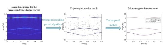
Figure 3a shows the range–time image when $SNR=10 \mathrm{dB}$ and the dwell time is 0.5 seconds. In this experiment, the scattering coefficients could be roughly estimated by the OMP algorithm, and the normalized estimated scattering coefficients were $a_1=0.09$, $a_2=1$ and $a_3=0.30$. Obviously, the echo energy scattered by $P_3$ was about 100 times than that scattered by the weak scattering center $P_1$. Figure 3b shows the trajectory extraction result by the OMP algorithm. We could find that there were many missing trajectories when the dwell time was 0.25 s, making the m-R track of $P_1$ disconnected.

Figure 3c,d shows the associated segments obtained by the AKF and the MKF, respectively. In these figures, curves in different colors represent different segments. The missing trajectory and the inaccurate estimation make the inlier radio decrease, and the new track is created by the RANSAC algorithm. Therefore, the track of $P_1$ obtained by the MKF is broken into two segments. Figure 4a–f shows the estimated range results and true ranges for different methods, respectively. The proposed method and the RANSAC algorithm can obtain accurate m-R estimation. ESPRIT cannot obtain an accurate m-R estimation of the weak scattering center $P_1$ under a low SNR circumstance. The wrong associations by the Kalman filter occur when the missing trajectories exist. The GRT-CLEAN and GA-CLEAN algorithms can obtain complete and accurate m-R curves, but they are restricted by the range resolution of the m-R image.

To evaluate the estimation accuracy and time cost of these methods, the mean variation of estimated root-mean-square errors (MRMSEs) with different SNRs and the time cost for different methods are given in

Table 2. MRMSE and time cost of m-R estimation when $\beta ={120}^{\circ }$. Results underlined indicate that the estimation results are the most accurate or time costs are the lowest, and results in bold indicate that the estimation results are the second-most accurate or the time costs are the lowest.

		9 dB	10 dB	11 dB	12 dB	15 dB	20 dB
MRMSE(m)	KALMAN	0.2377	0.2023	0.1962	0.1939	0.0374	0.0051
	RANSAC	0.0053	0.0053	0.0053	0.0052	0.0052	0.0050
	GRT-CLEAN	0.0236	0.0236	0.0235	0.0235	0.0235	0.0235
	GA-CLEAN	0.0239	0.0238	0.0238	0.0238	0.0238	0.0237
	AKF	0.0055	0.0054	5.4654 × 10−3	5.4306 × 10−3	5.3624 × 10−3	5.3401 × 10−3
	MKF	0.0193	0.0056	5.4865 × 10−3	5.4426 × 10−3	5.3652 × 10−3	5.3429 × 10−3
$R_{\mathrm{MKF}}-R_{\mathrm{AKF}}$(mm)		13.856	0.2089	0.0211	0.0120	0.0028	0.0028
Time cost(s)	KALMAN	0.0304	0.0328	0.0296	0.0300	0.0295	0.0329
	RANSAC	746.75	756.49	742.16	736.25	755.67	724.02
	GRT-CLEAN	56.022	55.987	55.951	55.847	56.006	55.919
	GA-CLEAN	19.063	19.092	19.110	19.053	19.008	19.028
	AKF	42.171	10.933	5.4887	2.9378	2.4502	2.4552
	MKF	61.758	21.7638	6.8817	3.0055	2.4649	2.4000
$T_{\mathrm{MKF}}-T_{\mathrm{AKF}}$(s)		19.5868	10.8309	1.3930	0.0677	0.0147	−0.0552

. The MRMSE can be obtained by

$$\mathrm{MRMSE}=\underset{i}{mean}\sqrt{\left({\displaystyle \sum _{i=0}^N{\left(r_t^i-{\widehat{r}}_t^i\right)}^2}\right)/N}$$

(20)

where $r_t^i$ denotes the true m-R of scatterer $P_i$ at $t$ time step and ${\widehat{r}}_t^i$ denotes the estimated m-R of scatterer $P_i$ at $t$ time step. Since the MRMSE of the proposed method and the MKF are approximate, we use the relative MRMSE and relative time cost to analyze the performance. The relative MRMSE can be calculated by $R_{\mathrm{MKF}}-R_{\mathrm{AKF}}$, where $R$ denotes the MRMSE, and relative time cost can be calculated by $T_{\mathrm{MKF}}-T_{\mathrm{AKF}}$, where $T$ denotes time cost. When the relative MRMSE and the relative time cost are positive, the proposed method has a better performance in estimation accuracy and time cost. Since the MKF cannot obtain a complete track, we use the RANSAC algorithm to process the segments and obtain the complete m-R tracks for the calculation of the relative MRMSE and time cost. In Table 2, results underlined indicate that the estimation results are the most accurate, or time costs are the lowest, and results in bold indicate that the estimation results are the second-most accurate, or the time costs are the lowest. ESPRIT cannot estimate the m-R of weak scattering center, so that we do not discuss this method in the table.

It is evident that the Kalman filter takes the least time, but its noise robustness is poor. Under the circumstance when $SNR\le 15 \mathrm{dB}$, it cannot associate trajectories correctly due to the influence of missing trajectories and spurious trajectories. GRT-CLEAN and GA-CLEAN algorithms obtain less accurate estimation results for relying on the resolution of the range–time image. The RANSAC can obtain the most accurate results, but the time cost of the RANSAC is far more than that of the proposed method. The proposed method can effectively deal with the missing trajectories and spurious trajectories problem, especially in the case of a low signal-to-noise ratio. In Table 2, the proposed method has a lower MRMSE than the MKF, especially under low SNR circumstances. When the $SNR\le 15 \mathrm{dB}$, the proposed method cost less time than the MKF. The proposed method can obtain a higher accuracy estimation and decline the wrong association probability, and the number of association corrections by the RANSAC algorithm is decreased, which significantly reduces time cost. When $SNR>15 \mathrm{dB}$, both the MKF and AKF can avoid the existence of the wrong association, and the calculation of prior error covariance in AKF brings a little more computational burden compared with the error covariance matrix estimation step in MKF. Therefore, the proposed method costs a little more time than the MKF. Overall, the proposed method has a better performance in both accuracy and time cost than other methods.

Experiment 2:

In this experiment, we set the target line-of-sight angle $\beta ={110}^{\circ }$. The trajectory of scattering center $P_1$ intersected with that of scattering center $P_2$.

Under the condition where the initial target line-of-sight angle is ${110}^{\circ }$, the range between the scattering center $P_1$ and the radar along the rLOS is close to that between the scattering center $P_2$, and the radar which makes the m-R tracks of two scattering centers intersected. Figure 5a shows the range–time image when $SNR=10 \mathrm{dB}$ and the dwell time was 0.5 s. Figure 5b shows the trajectory extraction result by the OMP algorithm. The intersection makes it difficult to associate the trajectories. Figure 5c,d shows the associated segments obtained by the AKF and the MKF, respectively. Obviously, the intersection increased the wrong association probability and made the track broken.

Figure 6a–f shows the estimated m-R results and the true m-R curves for different methods. It is obvious that there was a wrong association obtained by the Kalman filter near the intersection, which made the trajectory of the scattering center $P_1$ associate with the trajectory of the scattering center $P_2$. In the meantime, the trajectory of the scattering center $P_2$ was shaken near the intersection because of the influence of spurious trajectories. The proposed method and the RANSAC algorithm could obtain accurate m-R estimation. The ESPRIT algorithm could not obtain the correct estimation results for the influence of the weak signal power of scattering center $P_1$ and $P_2$. The Kalman filter obtained the wrong association near the intersection. The GRT-CLEAN and GA-CLEAN algorithms could obtain complete and accurate m-R curves, but they were restricted by the range resolution of the m-R image.

In

Table 3. MRMSE and time cost of m-R estimation when $\beta ={110}^{\circ }$. Results underlined indicate that the estimation results are the most accurate or the time costs are the lowest, and results in bold indicate that the estimation results are the sec-ond-most accurate or the time costs are the lowest.

		9 dB	10 dB	11 dB	12 dB	15 dB	20 dB
MRMSE(m)	KALMAN	0.9567	0.8315	0.4360	0.1600	0.0750	0.0715
	RANSAC	0.0026	0.0024	0.0023	0.0023	0.0023	0.0023
	GRT-CLEAN	0.0271	0.0271	0.0271	0.0270	0.0270	0.0270
	GA-CLEAN	0.0259	0.0259	0.0256	0.0257	0.0254	0.0250
	AKF	0.0034	0.0034	0.0034	0.0032	0.0031	3.1952 × 10−3
	MKF	0.0442	0.0151	0.0037	0.0034	0.0032	3.2375 × 10−3
$R_{\mathrm{MKF}}-R_{\mathrm{AKF}}$(mm)		40.775	11.660	0.3432	0.2241	0.0572	0.0423
Time cost(s)	KALMAN	0.0297	0.0301	0.0293	0.0302	0.0323	0.0294
	RANSAC	771.16	769.49	764.25	789.23	775.22	762.21
	GRT-CLEAN	55.642	55.666	55.549	55.625	55.632	55.652
	GA-CLEAN	19.146	19.145	19.079	19.085	19.069	19.062
	AKF	57.814	20.251	11.119	9.7701	8.3932	8.3796
	MKF	78.855	29.787	12.588	10.314	8.3570	8.2540
$T_{\mathrm{MKF}}-T_{\mathrm{AKF}}$(s)		21.041	9.5364	1.4689	0.5443	−0.0362	−0.1256

, results underlined indicate that the estimation results are the most accurate or the time costs are the lowest, and results in bold indicate that the estimation results are the second-most accurate or the time costs are the lowest. As is shown in this table, the Kalman filter cannot correctly associate the trajectories near the intersections in all cases of SNR, even if it costs the least time. The GRT-CLEAN and the GA-CLEAN can extract m-R curves, but the low range resolution of the range–time image will result in poor accuracy of parameter searching, and m-R estimation accuracy will be worse. The OMP algorithm in the proposed method can obtain a super-resolution m-R estimation result. Therefore, the estimation accuracy of GRT-CLEAN and the GA-CLEAN is not as good as that of our algorithm. The time cost of the RANSAC is far more than that of the proposed method. The AKF has a better performance on estimation accuracy than the MKF, and the AKF cost less time in a low SNR circumstance. When the signal-to-noise ratio is reduced, the proposed method guarantees accurate estimation results while costing only a small amount of time. In summary, its performance for estimation and time cost is significantly better than other traditional methods.

Experiment 3:

The influence of different process noise covariance matrixes on the estimation accuracy of the AKF and the MKF.

In this experiment, the SNR of echoes were set to be 10 dB and the initial target line-of-sight angle was $\beta ={120}^{\circ }$. The process noise covariance matrixes were $R_n=\mathrm{diag}(q,q)$, where $q$ denotes the diagonal element of the $R_n$ and $q$ is set to range from 0.1 to 1. We used two sets of data, where the precession rates were set to be $w_c=4\pi \mathrm{rad}/\mathrm{s}$ and $w_c=6\pi \mathrm{rad}/\mathrm{s}$. Figure 7 shows the range–time image when the precession rates were $w_c=4\pi \mathrm{rad}/\mathrm{s}$ and $w_c=6\pi \mathrm{rad}/\mathrm{s}$, respectively. We found that the m-R tracks on $w_c=4\pi \mathrm{rad}/\mathrm{s}$ were smoother than those on $w_c=6\pi \mathrm{rad}/\mathrm{s}$. Therefore, the theoretical diagonal element of the process noise covariance matrix should be larger when $w_c=6\pi \mathrm{rad}/\mathrm{s}$. Figure 8 shows the MRMSE of the AKF and MKF with different process noise covariance matrixes, where the blue markers show the MRMSE of the MKF and the red markers show the MRMSE of the AKF. In Figure 8a, the MRMSE is smallest when the noise variance of MKF is $R_n=\mathrm{diag}(0.6,0.6)$, indicating that $q=0.6$ is closest to the theoretical noise variance when $w_c=4\pi \mathrm{rad}/\mathrm{s}$. Since the calculation of the AKF does not need the noise variance, the MRMSEs with different process noise covariance are the same, and the MRMSE of the AKF is lower than that of the MKF. In Figure 8b, the MRMSE is the smallest when the noise variance of MKF is $R_n=\mathrm{diag}(0.7,0.7)$, indicating that $q=0.7$ is closest to the theoretical noise variance when $w_c=6\pi \mathrm{rad}/\mathrm{s}$, which is a little larger than when $w_c=4\pi \mathrm{rad}/\mathrm{s}$. The experimental results demonstrate that the AKF can obtain higher estimation accuracy than the MKF with different process noise covariance matrixes.

Experiment 4:

In this experiment, we compared the performance of the RANSAC and other variants.

In this experiment, the initial target line-of-sight angle was $\beta ={120}^{\circ }$. Other parameters are listed in Table 1 of the original paper. We used the AKF to obtain the associated segments and used the RANSAC, the MLESAC, and the R-RANSAC to connect the segments, respectively. As the GOODSAC and the locally optimized RANSAC were not are not applicable, we did not discuss and compare these two methods in this experiment. The MRMSE and time cost are provided in

Table 4. MRMSE and time cost of the RANSAC, the MLESAC, and the R-RANSAC.

		9 dB	10 dB	11 dB	12 dB	15 dB	20 dB
MRMSE(m)	MLESAC	0.0054	0.0054	0.0053	0.0053	0.0053	0.0053
	RANSAC	0.0054	0.0054	0.0053	0.0053	0.0053	0.0053
	R-RANSAC	0.0078	0.0061	0.0053	0.0053	0.0053	0.0053
$R_{\mathrm{RANSAC}}-R_{\mathrm{MLESAC}}$(m)		0.742 × 10−6	0.004 × 10−6	0.001 × 10−6	0	0	0
Time cost(s)	MLESAC	3.5614	3.2568	1.7424	1.5443	1.5203	1.1494
	RANSAC	3.2700	3.1342	1.6425	1.4562	1.4269	1.0216
	R-RANSAC	3.1277	3.0191	1.5948	1.4259	1.4176	1.0077

:

As is shown in Table 4, the MMRSE of the MLESAC and the RANSAC is the same because almost all the outliers were filtered out in the associated step by the AKF. However, the time cost of MLESAC is more than that of RANSAC for the calculation of probability distribution of error by inlier and outlier. The R-RANSAC costs less time because of the preliminary test. However, the test may reject the inlier segment, which makes the method less robust. In the proposed method, the cost time of the associated step of the AKF is far more than that of the connected step by RANSAC. To obtain precise and robust results, the RANSAC algorithm is chosen to associate the segments.

5. Conclusions

In this paper, we proposed a micro-Range estimation method combining the AKF and the RANSAC algorithm for a cone-shaped space target. To solve the unknown noise covariance problem and obtain complete m-R tracks in a low SNR circumstance, the AKF, which does not rely on the covariance matrix of process noise, was applied to associate the trajectories, and the RANSAC algorithm was used to obtain the complete m-R tracks by estimating the parameters of each m-R track. Compared with the MKF, the proposed method could obtain more accurate estimation results and complete m-R tracks. Compared with the Kalman filter and ESPRIT, the proposed method had a better performance on noise robustness and estimation accuracy. Compared with the GRT-CLEAN and GA-CLEAN methods, the proposed method had a fewer computational burden and obtained more precise estimation results. The proposed method can be applied in post-processing of ISAR image formation to improve precision and robustness. Its application in the imaging of a cone-shaped target and other space targets, such as rotating space debris, is part of our future research.