Motion Estimation Using Region-Level Segmentation and Extended Kalman Filter for Autonomous Driving

Abstract

Motion estimation is crucial to predict where other traffic participants will be at a certain period of time, and accordingly plan the route of the ego-vehicle. This paper presents a novel approach to estimate the motion state by using region-level instance segmentation and extended Kalman filter (EKF). Motion estimation involves three stages of object detection, tracking and parameter estimate. We first use a region-level segmentation to accurately locate the object region for the latter two stages. The region-level segmentation combines color, temporal (optical flow), and spatial (depth) information as the basis for segmentation by using super-pixels and Conditional Random Field. The optical flow is then employed to track the feature points within the object area. In the stage of parameter estimate, we develop a relative motion model of the ego-vehicle and the object, and accordingly establish an EKF model for point tracking and parameter estimate. The EKF model integrates the ego-motion, optical flow, and disparity to generate optimized motion parameters. During tracking and parameter estimate, we apply edge point constraint and consistency constraint to eliminate outliers of tracking points so that the feature points used for tracking are ensured within the object body and the parameter estimates are refined by inner points. Experiments have been conducted on the KITTI dataset, and the results demonstrate that our method presents excellent performance and outperforms the other state-of-the-art methods either in object segmentation and parameter estimate.

1. Introduction

Research on autonomous vehicles is being in the ascendant [1,2,3]. Autonomous Vehicles are cars or trucks that operate without human drivers, using a combination of sensors and software for navigation and control [4]. Autonomous vehicles require not only detecting and locating moving objects but also knowing their motion state relative to the ego-vehicle, i.e., motion estimation [5,6,7]. Motion estimation is a benefit to predict where other traffic participants will be at a certain period of time, and accordingly plan the route of the ego-vehicle. In this work, we propose a novel approach to estimate the motion state for autonomous vehicles by using region-level segmentation and Extended Kalman Filter (EKF).

Motion estimation involves three stages of object detection, tracking, and estimate of motion parameters including position, velocity, and acceleration in three directions. Accurate object detection is crucial for the high quality of motion estimation because the late two stages rely on the points within the object region; that is, only the points exactly within the object region can be used for tracking and parameter estimate. Existing works on motion estimation such as Refs. [8,9,10,11,12,13,14,15] normally generate bounding boxes as object proposals for the late two stages. One inherent problem of these methods is that the bounding boxes contain substantial background points as shown in Figure 1. These points are noise points and will result in unreliable object tracking and incorrect parameter estimate. To address this issue, we adopt two strategies: (1) Instead of bounding boxes, we use segmented object regions as object proposals. We employ the YOLO-v4 detector [16] to generate object bounding boxes and apply a region-level segmentation on them to accurately locate object contour and determine points within the objects (Figure 1 shows the results). (2) We compose an edge-point constraint on the feature points and apply the random sample consensus (RANSAC) [17] algorithm to eliminate outliers of tracking points so that the points used for tracking are ensured within the object body and the parameter estimate are refined by inner points. By the above processing, we can obtain a high-quality point set for tracking and parameter estimate, thereby generating accurate motion estimation.

Other aspects affecting motion estimation are how to establish the motion model for tracking and how to optimize the parameter estimate. In this work, we use optical flow to track the feature points. We propose a relative motion model of the ego-vehicle and moving objects, and accordingly establish an EKF model for point tracking and parameter estimate. The EKF model takes the ego-motion into considerations and integrates optical flow, and disparity to generate optimized object position and velocity.

In summary, we propose a novel framework for motion estimation by using region-level segmentation and Extended Kalman Filter. The main contributions of the work are:

• A region-level segmentation is proposed to accurately locate object regions. The proposed method segments object from a pre-generated candidate region, and refines it by combining color, temporal (optical flow), and spatial (depth) information using super-pixels and Conditional Random Field.
• We propose a relative motion model of the ego-vehicle and the object, and accordingly establish an EKF model for point tracking and parameter estimate. The EKF model integrates the ego-motion, optical flow, and disparity to generate optimized motion parameters.
• We apply edge-point constraint, consistency constraint, and the RANSAC algorithm to eliminate outliers of tracking points, thus ensuring that the feature points used for tracking are within the object body and the parameter estimates are refined by inner points.
• The experimental results demonstrate that our region-level segmentation presents excellent segmentation performance and outperforms the state-of-the-art segmentation methods. The motion estimation experiments confirm the superior performance of our proposed method over the state-of-the-art approaches in terms of the root mean squared error.

The remainder of this paper is organized as follows: Section 2 briefly introduces the relevant works. Section 3 describes the details of the proposed method including object detection and segmentation, and tracking and parameter estimate. The experiments and results are presented and discussed in Section 4. Section 5 concludes the paper.

2. Related Work

Motion estimation involves three stages of object detection, tracking, and estimate of motion parameters. The third stage that is served by the first two stages is the core of the whole pipeline. Thus, we divide the existing works on motion estimation into three categories in terms of the parameter estimates method, i.e., Kalman filter (KF)-based, camera ego-motion-based, and learning-based method.

The Kalman filter is an optimal recursive data processing algorithm that improves the accuracy of state measurement by fusion of prediction and measurement values. The KF-based method [10,11,12,18,19,20] generates optimized motion parameters by iteratively using a motion state equation for prediction and a measurement equation for updating. During the iteration, estimation error covariance is minimized. Lim, et al. [10] proposed an inverse perspective map-based EKF to estimate the relative velocity via predicting and updating the motion state recursively. The stereovision was used to detect moving objects, and the edge points within the maximum disparity region were extracted as the feature points for tracking and parameter estimate. Liu, et al. [11] combined Haar-like intensity features of the car-rear shadows with additional Haar-like edge features to detect vehicles, adopted an interacting multiple model algorithm to track the detected vehicles and utilized the KF to update the information of the vehicles including distances and velocities. Vatavu, et al. [12] proposed a stereo vision-based approach for tracking multiple objects in crowded environments. The method relied on measurement information provided by an intermediate occupancy grid and on free-form object delimiters extracted from this grid. They adopted a particle filter-based mechanism for tracking, in which each particle state is described by the object dynamic parameters and its estimated geometry. The object dynamic properties and the geometric properties are estimated by importance sampling and a Kalman Filter. Garcia, et al. [18] presented a sensor fusion approach for vehicle detection, tracking, and motion estimation. The approach employed an unscented Kalman filter for tracking and data association (fusion) between the camera and laser scanner. The system relied on the reliability of laser scanners for obstacle detection and computer vision technique for identification. Barth and Franke [19] proposed a 3-D object model by fusing stereovision and tracked image features. Starting from an initial vehicle hypothesis, tracking and estimate are performed by means of an EKF. The filter combines the knowledge about the movement of the object points with the dynamic model of a vehicle. He, et al. [20] applied an EKF for motion tracking with an iterative refinement scheme to deal with observation noise and outliers. The rotational velocity of a moving object was computed by solving a depth-independent bilinear constraint, and the translational velocity was estimated by solving a dynamics constraint that reveals the relation between scene depth and translational motion.

The camera ego-motion-based method [9,13,14,21] derives motion states of moving objects from camera ego-motion and object motion information relative to the camera. It generally consists of two steps: the first step is to obtain the camera’s ego-motion, and the second step is to estimate the object’s motion state by fusing the camera’s ego-motion with other object’s motion cues (such as relative speed, optical flow, depth, etc.). Kuramoto, et al. [9] obtained the camera ego-motion from the Global Navigation Satellite System/Inertial Measurement Unit. A framework using a 3-D camera model and EKF was designed to estimate the object’s motion. The output of the camera model was interlay utilized to calculate the measurement matrix of the EKF. The matrix was designed to map be-tween the position measurement on the objects in the image domain and the corresponding vector state in the real world. Hayakawa, et al. [13] predicted 2D flow by PWC-Net and detected the surrounding vehicles’ 3D bounding box using a multi-scale network. The ego-motion was extracted from the 2D flow using projection matrix and ground plane corrected by depth information. A similar approach was used for the estimation of the relative velocity of surrounding vehicles. The absolute velocity was derived from the combination of the ego-motion and the relative velocity. The position and orientation of surrounding vehicles were calculated by projecting the 3D bounding box into the ground plane. Min and Huang [14] proposed a method of detecting moving objects from the difference between the mixed flow (caused by both camera motion and object motion) and the ego-motion flow (evoked by the moving camera). They established the mathematical relationship between optical flow, depth, and camera ego-motion. Accordingly, a visual odometer was implemented for the estimation of ego-motion parameters by using ground points as feature points. The ego-motion flow was calculated from the estimated ego-motion parameters. The mixed flow was obtained from the correspondence matching between consecutive images. Zhang, et al. [21] presented a framework to simultaneously track the camera and multiple objects. The 6-DoF motions of the objects, as well as the camera, are optimized jointly with the optical flow in a unified formulation. The object velocity was calculated using the rotation and translation part of the motion of points in the global reference frame. The proposed framework detected moving objects via combining Mask R-CNN object segmentation [22] and scene flow, and tracked them over frames using optical flow.

Different from the first two categories of the methods, the learning-based method [8,15,23,24] does not require a specific mathematical estimation model but relies on ma-chine learning and the ability of neural network regression to estimate the motion parameters. Jain, et al. [8] used Farneback’s algorithm to calculate optical flow and the DeepSort algorithm to track vehicles detected from the YOLO-v3. The optical flow and the tracking information of the vehicle were then treated as input for two different networks. The features extracted from the two networks were stacked to create a new input for a lightweight Multilayer Perceptron architecture which finally predicts positions and velocities. Cao, et al. [15] presented a network for learning motion parameters from stereo videos. The network masked object instances and predicted specific 3D scene flow maps, from which the motion direction and speed for each object can be derived. The network took the 3D geometry of the problem into account which allows it to correlate the input images. Kim, et al. [23] developed a deep neural network that exploits different levels of semantic information to perform the motion estimation. The network used a multi-context pooling layer that integrates both object and global features, and adopt the cyclic ordinal regression scheme using binary classifiers for effective motion classification. In the detection stage, they ran the YOLO-v3 detector to obtain the bounding boxes. Song, et al. [24] presented an end-to-end deep neural network for estimation of inter-vehicle distance and relative velocity. The network integrated multiple visual clues provided by two time-consecutive frames, which include deep feature clue, scene geometry clue, as well as temporal optical flow clue. It also used a vehicle-centric sampling mechanism to alleviate the effect of perspective distortion in the motion field.

Moving object detection is a prerequisite for motion estimation. Most of the existing methods use bounding boxes as object proposals which affect the accuracy of the motion estimation for the late two stages. In this study, we leverage a region-level segmentation to accurately locate object regions for tracking and parameter estimate. Therefore, we review here relevant segmentation works compared with our segmentation methods. PSPNet [25] is a pyramid scene parsing network based on the full convolution network [26], which exploits the capability of global context information by different-region-based context aggregation. PSPNet can provide a pixel-level prediction for the scene parsing task. Mask R-CNN [22] is a classic network for object instance segmentation. It extends Faster R-CNN by adding a branch in parallel with the existing detection branch for predicting object masks. Bolya, et al. [27,28] proposed the YOLACT series, a fully convolutional model for real-time instance segmentation. YOLACT series break instance segmentation into two parallel subtasks, generating a set of prototype masks and predicting per-instance mask coefficients, to achieve compromise of segmentation quality and computation efficiency.

3. Method

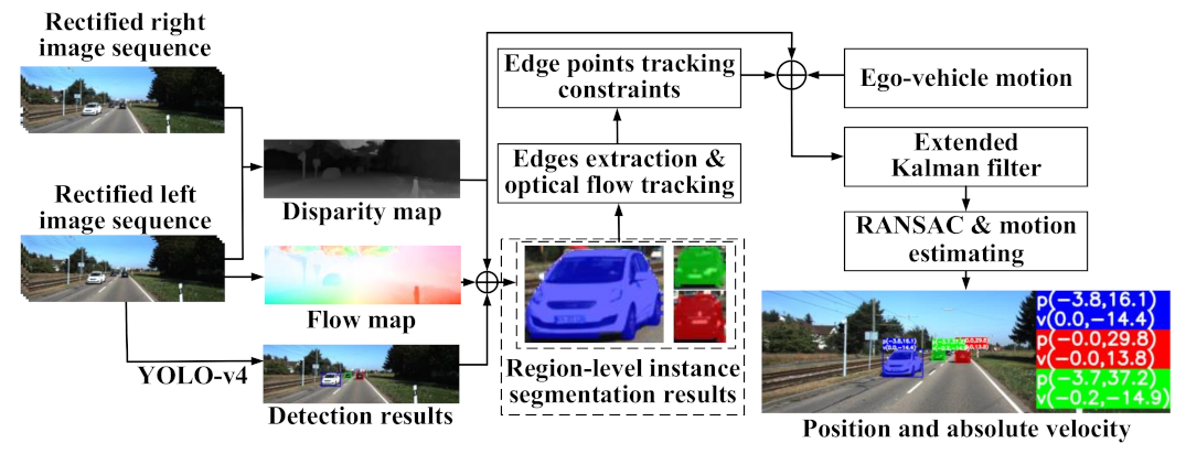
The framework of the proposed method is shown in Figure 2. The main idea is to accurately determine feature points within the object through instance segmentation and predict the motion state by tracking the feature points through an EKF. The method includes two stages: (1) object segmentation, (2) tracking and motion estimate.

In the first stage, we use the YOLO-v4 detector to locate the object region in a form of a bounding box, and then extract accurate object contour through a region-level segmentation. The output is the feature points exactly within the object body.

In the second stage, we compose an edge-point constraint to further refine the feature points. We use Optical Flow to track the refined feature points. We propose a relative motion model with respect to the ego-vehicle and a moving object, and accordingly establish an EKF model for parameter estimation. We also apply the random sample consensus (RANSAC) algorithm to eliminate outliers of the tracked points. The EKF model integrates the ego-motion, optical flow, and disparity to generate optimized object position and velocity.

3.1. Object Detection and Region-Level Segmentation

Object detection is to locate the object region while segmentation is to determine foreground pixels (the object body) within the region. Figure 3 shows a process of object detection and segmentation.

We employ a YOLO-v4 detector to locate the object region. The details of YOLO-v4 can be found in Reference [16]. The detection result is in a form of a bounding box contains background, as shown in Figure 3a.

Region-level segmentation consists of three stages including Grabcut, Super-pixels, and Super-pixels fixed by Conditional Random Field. Starting from the bounding box (Figure 3a) detected by YOLO-v4, we apply the GrabCut algorithm to segment foreground from background. GrabCut algorithm proposed in Ref. [29] is an interactive method that segments images according to texture and boundary information. When using GrabCut, we initially define the inner of the bounding box as foreground and the external as background, and accordingly build a pixel-level Gaussian Mixture Model to estimate the texture distribution of foreground/background. By an iterative process until convergence, we can obtain the confidence maps of the foreground and background. The results are shown in Figure 3b,c.

Accordingly, GrabCut assigns a label $({\gamma }_{uv})$ to pixel $\left(u,v\right)$ as follows:

$${\gamma }_{uv}=\left\{\begin{array}{c}1, \mathrm{if} \left(u,v\right) \mathrm{is}\mathrm{foreground}\\ 0, \mathrm{if} \left(u,v\right) \mathrm{is} \mathrm{background}\end{array}\right.$$

(1)

The result is shown in Figure 3d in which the background is marked as black and the foreground is marked as red. This is a pre-segmentation process with some significant errors, for example, the license plate in Figure 3d is excluded from the car body.

We refine the pre-segmentation in virtue of Super-pixels idea proposed in Reference [30]. Super-pixels are an over-segmentation formed by grouping pixels based on low-level image properties including color, brightness, etc. Super-pixels provide a perceptually meaningful tessellation of image content, and naturally preserve the boundary of objects, thereby reducing the number of image primitives for subsequent segmentation. We adopt Simple Linear Iterative Clustering (SLIC) [31] to generate M super-pixels. SLIC is a simple-minded and easy-to-implement algorithm. It transforms the color image to CIELAB color space, constructs the distance metric based on coordinates and L/A/B color components, and adopts the k-means clustering approach to efficiently generate super-pixels. The label ${\vartheta }_{s_{\beta }}$ of a super-pixel $s_{\beta }$ is marked by Equation (2):

$${\vartheta }_{s_{\beta }}=\left\{\begin{array}{c}1, {\displaystyle {\displaystyle \sum }_{\left(u,v\right)\in s_{\beta }}}{\gamma }_{uv}\ge \frac{num}{2}\hfill \\ 0, \mathrm{other}\hfill \end{array}\right.$$

(2)

where $num$ is the total number of pixels within super-pixel $s_{\beta }$. The generated super-pixels are shown in Figure 3e where the white lines partition the super-pixels. Super-pixels can greatly reduce computation load in the late stages.

Conditional Random Field (CRF) [32] is a discriminative probability model and is often used in pixel labeling. Supposing the output random variable constitutes a Markov random field, CRF is the extension of the maximum entropy Markov model. Since the labels of super-pixels can be regarded as such a random variable, we can use CRF to model the labeling problem. We define the CRF as an undirected graph with super-pixels as nodes. It can be solved through an approximate graph inference algorithm by minimizing an energy function. The energy function generally contains a unary potential and a pairwise potential. The unary potential is only related to the node itself and determines the likelihood of the node to be labeled as a class. The pairwise potential describes the interactions between neighboring nodes, and is defined as similarity between them. In this work, we employ CRF to fix the labels of super-pixels generated in Figure 3e. Two super-pixels are considered as neighbors if they share an edge in image space. Let $s_{\beta }$ and ${\mathrm{s}}_j$ ($\beta , j=1,2,\cdots ,M$) be neighboring super-pixels, the CRF energy function is defined as

$$E_{seg}\left(\Theta \right)={\displaystyle \sum }_{s_{\beta }}{\varnothing }_u\left(s_{\beta },{\vartheta }_{s_{\beta }}\right)+{\displaystyle \sum }_{(s_{\beta },s_j)\in \epsilon }{\varnothing }_p\left(s_{\beta },s_j\right)$$

(3)

where $\epsilon$ denotes the set of all neighboring super-pixels. ${\vartheta }_{s_{\beta }}$ is the initial super-pixel label assigned in Equation (2). $\Theta$ represents the 1/0 labeling of super-pixels. The energy function is minimized by using graph cuts algorithm. We refer readers to [33] for a detailed derivation of the minimization algorithm.

The unary potential ${\varnothing }_u\left(s_{\beta },{\vartheta }_{s_{\beta }}\right)$ in Equation (3) measures the cost of labeling $s_{\beta }$ with ${\vartheta }_{s_{\beta }}$:

$${\varnothing }_u\left(s_{\beta },{\vartheta }_{s_{\beta }}\right)=\left\{\begin{array}{c}-log\left(CO{F}_{fg}\left(s_{\beta }\right)\right), if {\vartheta }_{s_{\beta }}=1\\ -log\left(CO{F}_{bg}\left(s_{\beta }\right)\right), if {\vartheta }_{s_{\beta }}=0\end{array}\right.$$

(4)

where $CO{F}_{fg}\left(s_{\beta }\right)$ denotes the probability that $s_{\beta }$ belongs to the foreground, computed by averaging the foreground confidence scores (Figure 2b) over all pixels in $s_{\beta }$. $CO{F}_{bg}\left(s_{\beta }\right)$ is the probability that $s_{\beta }$ belongs to the background.

The pairwise potential ${\varnothing }_p\left(s_{\beta },s_j\right)$ in Equation (3) describes the interaction relationship between two neighboring super-pixels. ${\varnothing }_p\left(s_{\beta },s_j\right)$ incorporates the pairwise constraint by combining color similarity, the mean optical flow direction similarity and the depth similarity between $s_{\beta }$ and $s_j$. ${\varnothing }_p\left(s_{\beta },s_j\right)$ is defined as

$$\{\begin{array}{c}{\varnothing }_p\left(s_{\beta },s_j\right)=\lambda \mathbf{1}\left({\vartheta }_{s_{\beta }}\ne {\vartheta }_{s_j}\right)·D_{lab}\left(s_{\beta },s_j\right)·D_{flow}\left(s_{\beta },s_j\right)·D_{depth}\left(s_{\beta },s_j\right)\hfill \\ D_{lab}\left(s_{\beta },s_j\right)=1/\left(1+\Vert lab\left(s_{\beta }\right)-lab{\left(s_j\right)\Vert }_2\right)\hfill \\ D_{flow}\left(s_{\beta },s_j\right)=F{L}_{s_{\beta }}F{L}_{s_j}/(\Vert F{L}_{s_{\beta }}{\Vert }_2\Vert F{L}_{s_j}{\Vert }_2)\hfill \\ D_{depth}\left(s_{\beta },s_j\right)={\displaystyle \sum }\sqrt{his{t}_{s_{\beta }}\times his{t}_{s_j}}\hfill \end{array}$$

(5)

where $\lambda$ is the weight used to adjust the pairwise potential function in $E_{seg}$. $\mathbf{1}\left(·\right)$ is an indicator function: if the input condition is true, the output is 1; otherwise, the output is 0. ${\Vert ·\Vert }_2$ denotes the L 2-norm. $D_{lab}\left(s_{\beta },s_j\right)$ defines the color similarity between $s_{\beta }$ and $s_j$. $lab\left(s_{\beta }\right)$ is computed as the average LAB color of $s_{\beta }$ in CIELAB color space. $F{L}_{s_{\beta }}$ is the mean optical flow of $s_{\beta }$ and $D_{flow}\left(s_{\beta },s_j\right)$ represents the direction similarity between the mean flows of $s_{\beta }$ and $s_j$. $D_{depth}\left(s_{\beta },s_j\right)$ is the depth similarity between $s_{\beta }$ and $s_j$, measured using the Bhattacharyya distance. $his{t}_{s_{\beta }}$ is the normalized depth histogram of $s_{\beta }$. It can been seen that the pairwise potential integrates color, temporal (optical flow) and spatial (depth) information as criteria for segmentation purpose. The final segmentation result is shown in Figure 3f.

3.2. Tracking and Parameter Estimate

We use Optical Flow to track the feature points. We establish a relative motion model between ego-vehicle and object by taking camera ego-motion into considerations, accordingly build an EKF model for point tracking and parameter estimate. The EKF model integrates the ego-motion, optical flow, and disparity to generate optimized object position and velocity. During the tracking process, we compose an edge-point constraint to refine the feature points. During the parameter estimate, we apply the RANSAC algorithm to eliminate outliers of tracked points.

3.2.1. The Relative Motion Model of the Ego-Vehicle and the Object

Figure 4 shows the relative motion model between the ego-vehicle and a moving object.

The ego-vehicle and the object move on X-Z plane. Assuming that the ego-vehicle moves from position C₁ to C₂ within a time interval $\mathsf{\Delta }\mathit{t}$ with a translational velocity $V^S={\left[V_X^S,V_Y^S,V_Z^S\right]}^T$ and a rotational velocity around Y-axis ${\omega }^S$, the trajectory can be regarded as the arc C₁C₂ with a rotation angle $\alpha ={\omega }^S\times \mathsf{\Delta }\mathrm{t}$. The displacement $\mathsf{\Delta }{\mathit{L}}^S={\left[\mathsf{\Delta }{X}^S,0,\mathsf{\Delta }{Z}^S\right]}^{\mathit{T}}$ in the camera coordinates at position C₂ will be:

$$\mathsf{\Delta }{\mathit{L}}^S=\left[\begin{array}{c}\mathsf{\Delta }{X}^S\\ 0\\ \mathsf{\Delta }{Z}^S\end{array}\right]=\frac{\Vert {\mathit{V}}^S{\Vert }_2}{{\omega }^S}\left[\begin{array}{c}1-cos\alpha \\ 0\\ -sin\alpha \end{array}\right]$$

(6)

The object P is located at C₃ at time t, and the absolute velocities in the camera coordinates at position C₁ is ${\mathit{V}}_t^O={\left[V_{Xt}^O,V_{Yt}^O,V_{Zt}^O\right]}^T$. Assuming that the object moves from C₃ to C₄ with ${\mathit{V}}_t^O$ within $\mathsf{\Delta }\mathit{t}$, the absolute velocities ${\mathit{V}}_{t+\mathsf{\Delta }\mathit{t}}^O$ of P at time $t+\mathsf{\Delta }\mathrm{t}$ is related to the change of the camera coordinates. Taking ego-vehicle motion into considerations, the displacement $\mathsf{\Delta }{\mathit{L}}^O$ and ${\mathit{V}}_{t+\mathsf{\Delta }t}^O$ of P in the camera coordinates at C₂ are computed from:

$$\mathsf{\Delta }{\mathit{L}}^O={\mathit{V}}_{t+\mathsf{\Delta }\mathit{t}}^O\times \mathsf{\Delta }\mathit{t}$$

(7)

$${\mathit{V}}_{t+\mathsf{\Delta }\mathit{t}}^O=\mathit{R}\left(\alpha \right){\mathit{V}}_t^O$$

(8)

where $\mathit{R}\left(\alpha \right)$ is the rotation matrix given by the Rodrigues rotation formula:

$$\mathit{R}\left(\alpha \right)=\left[\begin{array}{ccc}cos\alpha & 0& -sin\alpha \\ 0& 1& 0\\ sin\alpha & 0& cos\alpha \end{array}\right]$$

(9)

Thus, given the coordinates of P in the camera coordinates at C₁ at time t ${\mathit{P}}_t={\left[X_t,Y_t,Z_t\right]}^T$, the coordinates of P in the camera coordinates at C₂ at time $t+\mathsf{\Delta }\mathit{t}$ ${\mathit{P}}_{t+\mathsf{\Delta }\mathit{t}}$ is calculated by:

$${\mathit{P}}_{t+\mathsf{\Delta }t}=\mathit{R}\left(\alpha \right)\times {\mathit{P}}_t+\mathsf{\Delta }{\mathit{L}}^O+\mathsf{\Delta }{\mathit{L}}^S$$

(10)

3.2.2. Design of Kalman Filter

(1) Motion Model

The state vector for P is defined as

$$\mathit{S}\mathit{V}={\left[X,Y,Z,V_X^O,V_Y^O,V_Z^O\right]}^T$$

(11)

where ${\left[X,Y,Z\right]}^T$ represents the coordinates of P in the moving camera coordinates. ${\left[V_X^O,V_Y^O,V_Z^O\right]}^T$ is the absolute velocities of P moving along the X-axis, Y-axis and Z-axis.

Combing Equations (6) – (8) and (10), The time-discrete motion equation for the state vector $\mathit{S}\mathit{V}$ is given by:

$$\mathit{S}{\mathit{V}}_k=\mathit{A}\times \mathit{S}{\mathit{V}}_{k-1}+{\mathit{B}}_{k-1}+{\delta }_k$$

(12)

$$\mathit{A}=\left[\begin{array}{cc}\mathit{R}\left(\alpha \right)& \mathsf{\Delta }\mathit{t}\times \mathit{R}\left(\alpha \right)\\ 0& \mathit{R}\left(\alpha \right)\end{array}\right]$$

(13)

$${\mathit{B}}_{k-1}=\frac{{\mathit{V}}_{k-1}^S}{{\omega }^S}\left[\begin{array}{c}1-cos\alpha \\ 0\\ -sin\alpha \\ 0\\ 0\\ 0\end{array}\right]$$

(14)

where k is the time index, the process noise ${\delta }_k$ is considered as Gaussian white noise with a mean value of zero.

(2) Measurement Model

The measurement vector for P is $\mathit{M}\mathit{V}={\left[u,v,d\right]}^T$ where $\left(u,v\right)$ is the projection, and d is the disparity. The optical flow is used to track $P_k\left(u,v\right)$ at time k to $P_{k+1}\left(u,v\right)$ at time k+1, and the corresponding disparities $d_k$ and $d_{k+1}$ can be measured from the stereovision.

According to the ideal pinhole camera model, the nonlinear measurement equation can be written as:

$$\mathit{M}{\mathit{V}}_k=\mathrm{H}\left(\mathit{S}{\mathit{V}}_k\right)+{ϵ}_k$$

(15)

$$H\left(\mathit{S}{\mathit{V}}_k\right)=\left\{\begin{array}{c}u=\frac{f_u\times X}{Z}+c_u\\ v=\frac{f_v\times Y}{Z}+c_v\\ d=\frac{b\times f_u}{Z}\end{array}\right.$$

(16)

where ${ϵ}_k$ is the Gaussian measurement noise. $f_u$, $f_v$ are the camera focal lengths; $c_u$, $c_v$ are the camera centre offsets and b is the camera baseline length. The Jacobian matrix of measurement equation can be expressed as

$$\mathit{J}=\left[\begin{array}{cccccc}\frac{f_u}{Z}& 0& -\frac{f_u\times X}{Z^2}& 0& 0& 0\\ 0& \frac{f_v}{Z}& -\frac{f_v\times Y}{Z^2}& 0& 0& 0\\ 0& 0& -\frac{b\times f_u}{Z^2}& 0& 0& 0\end{array}\right]$$

(17)

(3) Estimation and Update

The location and absolute velocities of P can be obtained by iterating the following estimation and update process. The time update equations are:

$$\mathit{S}{\mathit{V}}_k^{-}=\mathit{A}\times \mathit{S}{\mathit{V}}_{k-1}+{\mathit{B}}_{k-1}$$

(18)

$${\mathit{P}}_k^{-}=\mathit{A}{\mathit{P}}_{k-1}{\mathit{A}}^T+{\mathit{Q}}_k$$

(19)

where $\mathit{S}{\mathit{V}}_k^{-}$ is the priori estimate of the state vector $\mathit{S}\mathit{V}$ at time k, $\mathit{S}{\mathit{V}}_{k-1}$ is the posteriori estimate (optimal value) of the state vector $\mathit{S}\mathit{V}$ at time k-1, ${\mathit{P}}_k^{-}$ is the priori estimate of the variance of the estimation error, ${\mathit{Q}}_k$ is the covariance of ${\delta }_k$.

The measurement update equations are

$${\mathit{G}}_k={\mathit{P}}_k^{-}{\mathit{J}}_k^T{\left({\mathit{J}}_k{\mathit{P}}_k^{-}{\mathit{J}}_k^T+{\mathit{W}}_k\right)}^{-1}$$

(20)

$$\mathit{S}{\mathit{V}}_k=\mathit{S}{\mathit{V}}_k^{-}+{\mathit{G}}_k\left(\mathit{M}{\mathit{V}}_k-\mathrm{H}\left(\mathit{S}{\mathit{V}}_k^{-}\right)\right)$$

(21)

$${\mathit{P}}_k=\left(\mathit{I}-{\mathit{G}}_k{\mathit{J}}_k\right){\mathit{P}}_k^{-}$$

(22)

where ${\mathit{G}}_k$ is the Kalman gain, ${\mathit{W}}_k$ is the covariance of ${ϵ}_k$, I is the identity matrix, $\mathit{S}{\mathit{V}}_k$ is the posteriori estimate (optimal value) of the state vector $\mathit{S}\mathit{V}$ at time k, and ${\mathit{P}}_k$ is the posteriori estimate of the variance of the estimation error.

3.2.3. Feature-Point Filtering

The tracking discussed in the above EKF is for a single object point. As described in Section 3.1, each segmented object consists of a cluster of points, i.e., a set of foreground pixels. For sake of tracking reliability and computation efficiency, it is essential to select reliable feature points for tracking and estimation. The motion state of an object is taken as the average of these points. Feature-point filtering is crucial for tracking and estimation.

Since the edge points have a strong textural feature and facilitate optical flow calculations, we employ the Canny operator [34] to extract the edge points as feature points. During the tracking, we compose an edge-point constraint on the tracking results. That is, the tracked points must still be edge points, otherwise, they are excluded.

Furthermore, we enhance estimation accuracy by applying the RANSAC algorithm [17] to eliminate outliers of tracking points. The RANSAC is a statistics-based hypothesis-verification method that iteratively finds the inner data from noisy data. In each iteration, a minimum number of samples is randomly selected to construct a consistency hypothesis, and other samples are verified whether they conform to the hypothesis. The samples that conform are taken as inner samples. Repeat the above steps to form a sample set with the largest number of inner samples, i.e., the maximum consensus set, for calculation of the motion parameters.

We compose a consistency constrain on the estimate results, that is, the estimate results for feature points in the same object should be consistent. In this work, the longitudinal distance and velocity, the lateral distance and velocity are used as target parameters to iteratively select the inner data set. The implementation flow for the RANSAC filtering is illustrated in Algorithm 1.

Algorithm 1. Implementation flow for RANSAC filtering (example of longitudinal distance).

Input: A set of feature points: FR       The maximum iterations: $I_{max}$            Consistency threshold th, i.e., the threshold of the deviation that is the difference between longitudinal distance and its            average. Output: The maximum consensus set: ${\prod }_{max}$ The object longitudinal distance: ${\zeta }_{\mathrm{final}}$

$i=0$, $N_{max}=0$ while $i<I_{max}$do             1 Hypothesis generation             Randomly select m feature points form FR as minimal consensus set             Calculate the average longitudinal distance ${\zeta }_Z$ in the minimal consensus set             2 Verification             Calculate the difference between the longitudinal distance of each point in FR and ${\zeta }_Z$, i.e., deviations             Determine a set $F{R}_i$ whose deviations are less than th              Count the total number of $F{R}_i$ as N             If $N>N_{max}$ then             ${\prod }_{max}=F{R}_i$, $N_{max}=N$             end if             i = i + 1 end while             Calculate the average longitudinal distance in ${\prod }_{max}$ as ${\zeta }_{\mathrm{final}}$

4. Experiments

Experiments have been conducted on image sequences (Road and City) of the KITTI public datasets [35]. The binocular camera settings are: baseline length 0.54 m, mounting height 1.65 m, tilt angle to the ground 0°, and rectified image resolution 375 × 1242. KITTI provides the ground truth of ego-vehicle motion, motion state of moving objects. The experiments were implemented in the workstation with an Intel Xeon Silver 4110 4 core processor, 16GB RAM, a Nvidia GeForce gtx1080ti graphic processor, and 11 GB video memory.

We use HD³-flow [36] for predicting optical flow and employ PSMNet [37] to generate the disparity maps. We retrained HD³-flow and PSMNet based on the original weights using the KITTI dataset.

4.1. Segmentation Results

We compare our segmentation method with two state-of-the-art methods, PSPNet [25] and YOLACT++ [28]. The results of three methods compared with the ground truth are shown in Figure 5. The fourth row shows the results obtained by our method only using color information without using optical flow, and disparity, called “Our method^1”.

In the road scene, it can be seen that our method can accurately segment the Obj. 1, 2, and 3. Our method¹ fails in recognizing the license plates and lights of Obj. 2 and 3 as part of the car bodies. PSPNet wrongly mixtures Obj. 2 and 3 together while YOLACT++ wrongly mixtures distant building with Obj. 2 into one object.

In the city scene, our method also achieves the best result either in frame 4 (no-occlusion case) or frame 9 (occlusion case). Especially, our method is able to accurately distinguish Obj. 4 from the traffic light poles in frame 9. PSPNet presents significant errors either on frame 4 or frame 9 while YOLACT++ fails to segment Obj. 4 from the traffic poles. Our method¹ does not correctly segment the front windshield of Obj.4 in frame 9, while the wheels are excluded from the car body in frame 4 and 9.

We use four metrics to quantitatively evaluate the segmentation performance.

Mean Intersection over Union (MIoU) [38]: It computes a ratio between the intersection and the union of the ground truth and predicted segmentation.

$$\mathit{M}\mathit{I}\mathit{o}\mathit{U}=\frac{1}{l}{\displaystyle \sum }_{l_1=0}^1\frac{C{N}_{l_1{l}_1}}{{{\displaystyle \sum }}_{l_2=0}^{1}C{N}_{l_1{l}_2}+{{\displaystyle \sum }}_{l_2=0}^{1}C{N}_{l_2{l}_1}-C{N}_{l_1{l}_1}}$$

(23)

where $l$ is the class number, in this case $l=2$ (foreground/background). $C{N}_{l_1{l}_2}$ is the number of pixels of class $l_1$ inferred to belong to class $l_2$ and by parity of reasoning. When calculating MIoU, $l_1$ and $l_2$ are regarded as foreground (1) or background (0) respectively to count the positive and negative pixels. Thus, $l_1$ and $l_2$ refers to be 1 or 0.

The False Positive Rate (FPR) and the False Negative Rate (FNR) are computed by

$$FPR=\frac{FP}{FP+TN}$$

(24)

$$FNR=\frac{FN}{FN+TP}$$

(25)

where True Positive (TP) and False Positive (FP) indicate the correctly and incorrectly segmented positive (foreground) pixels, while the True Negative (TN) and False Negative (FN) indicate the correctly and incorrectly segmented negative (background) pixels.

Overall error (Ov. err.) is the percentage of wrongly labelled pixels.

Since the KITTI doesn’t provide the ground truth of the instance segmentation, we manually labeled 411 images from the Road and City sequences. We conducted experiments on those images, and the average values of the metrics are listed in

Table 1. Comparison of segmentation performance of three methods.

	MIoU (%)	FPR (%)	FNR (%)	Ov.err. (%)
PSPNet [25]	72.04	19.05	13.98	14.75
YOLACT++ [28]	84.37	11.09	4.57	7.51
Our method1	63.67	20.53	23.35	19.57
Our method	88.42	5.6	4.88	5.24

. It can be seen that our method achieves the best MIoU score and the lowest FPR, FNR, and Ov.err., and outperforms other methods.

The reasons for the superior performance of our method are: (1) our method segments object from candidate region (bounding box) pre-generated by YOLO-v4 detector rather than from the whole image, which eliminates trivial information and makes segmentation easy; (2) our method combines color, temporal (optical flow), and spatial (depth) information as the basis for segmentation; and (3) super-pixels naturally preserve the boundary of objects and are computationally efficient for processing.

4.2. Results of Feature-Point Filtering

As described in Section 3.2.3, the edge points within the object point cluster are used as feature points for tracking. The edge point constraint and consistency constraint are applied to filter the feature points. Taking a segmented object as an example, the filtering processing is shown in Figure 6. Figure 6a shows the point cluster obtained from our region-level segmentation, and Figure 6b shows the edge points extracted by the Canny operator, which are taken as feature points. The yellow points in Figure 6c are the feature points in Figure 6b (previous frame) that are tracked to the current frame while the white points are the edge points in the current frame. Some of the yellow points do not overlap the white points and should be eliminated. The blue points in Figure 6d are the result of excluding the non-overlapping points, i.e., satisfying the edge point constraint. The results of applying the consistency constraint on Figure 6d are shown in Figure 6e. The red points are the feature points with consistent distances and velocities that have been selected by the RANSAC, i.e., the maximum consensus set. The arrows in Figure 6f represent the optical flows of the valid feature points. It can be seen that the optical flows are identical, indicating a valid feature point selection.

4.3. Motion Estimate Results and Analysis

4.3.1. Motion Estimate Results

Table 2. Position and absolute velocity of objects in Figure 5 and their estimate errors.

		Estimates (E)				Ground Truth (GT)				Absolute Errors (e = E −GT)
Sequence	Obj.	${\mathit{X}}_{\mathit{E}}$ (m)	${\mathit{Z}}_{\mathit{E}}$ (m)	${\mathit{V}}_{\mathit{X}\mathit{E}}$ (m/s)	${\mathit{V}}_{\mathit{Z}\mathit{E}}$ (m/s)	${\mathit{X}}_{\mathit{T}}$ (m)	${\mathit{Z}}_{\mathit{T}}$ (m)	${\mathit{V}}_{\mathit{X}\mathit{T}}$ (m/s)	${\mathit{V}}_{\mathit{Z}\mathit{T}}$ (m/s)	${\mathit{e}}_{\mathit{X}}$ (m)	${\mathit{e}}_{\mathit{Z}}$ (m)	${\mathit{e}}_{{\mathit{V}}_{\mathit{X}}}$ (m/s)	${\mathit{e}}_{{\mathit{V}}_{\mathit{Z}}}$ (m/s)
Road scene (#frame 219)	1	−3.5	12.2	−0.2	−14.7	−3.6	12.3	−0.1	−14.4	0.1	−0.1	−0.1	−0.3
	2	0.0	30.5	0.0	12.7	0.0	30.8	0.0	12.9	0.0	−0.3	0.0	−0.2
	3	−3.5	37.9	0.0	−12.4	−3.5	37.5	−0.4	−13.0	0.0	0.4	0.4	0.6
City scene (#frame 4)	4	−10.1	15.7	10.7	−2.2	−9.9	15.9	11.0	−2.1	−0.2	−0.2	−0.3	−0.1
	5	8.1	12.0	10.5	−2.1	8.2	12.2	10.8	−2.2	−0.1	−0.2	−0.3	−0.1
City scene (#frame 9)	4	−4.6	14.7	11.2	−2.2	−4.5	15.0	11.0	−2.1	−0.1	−0.3	0.2	−0.1

lists the estimates and errors of position and absolute velocity of the objects in Figure 5. It can be seen that our method presents small errors. In the Road scene, objects have little variation in their lateral positions and mainly move longitudinally. The maximum absolute errors of the objects’ longitudinal position and velocity estimations are 0.4 m (Obj. 3, corresponding to the ground truth 37.5 m) and 0.6 m/s (Obj. 3, corresponding to −13.0 m/s), respectively. In the City scene, the objects are mainly moving laterally from left to right. The maximum absolute errors of the objects’ lateral position and velocity estimation are −0.2 m (Obj. 4 in frame 4, corresponding to −9.9 m) and −0.3 m/s (Obj. 5 in frame 4, corresponding to 10.8 m/s), respectively.

Figure 7 shows the results of object segmentation and motion estimation in three frames of the Road scene sequence. $P\left(X,Z\right)$ indicates the lateral and longitudinal distances of objects in the camera coordinates, while $V\left(V_X,V_Z\right)$ denotes the lateral and longitudinal absolute velocities. Starting from frame 210 to frame 291, the red car that moves in the same direction as the ego-vehicle is tracked. At frame 210, it is 29.8 m away from the ego-vehicle with a longitudinal velocity of 13.8 m/s. At frame 210, it is getting far with a distance of 33.9 m and a velocity of 15.2 m/s. At frame 291, it is getting closer with a distance of 32.3 m and a velocity of 13.7 m/s. At the same time, other vehicles on the road (as shown in the blue, green, brown, and purple masks) are also segmented, tracked and predicated with their motion states.

4.3.2. Evaluation and Comparison

We tested our method against the ground truth over a sequence of images. We evaluated our method in terms of: (1) the method with feature-point filtering (w Ft.Pts.F.); (2) the method without feature-point filtering (w/o Ft.Pts.F.). Figure 8 shows the variations of lateral distance and velocity of Obj. 4 from frame 4 to 23 in the City scene. It moves almost uniformly from left to right, the lateral distance becomes progressively larger and the lateral absolute velocity is approximately constant. Figure 9 shows the variations of longitudinal distance and velocity of Obj. 2 from frame 4 to 294 in the Road scene. It moves in the same direction as the ego-vehicle. It can also be seen that the variations of the w Ft.Pts.F. method are closer to the ground truth and smoother than the w/o Ft.Pts.F. method. This indicates that the performance of our method is improved by using feature-point filtering.

There is no uniform evaluation metric for object motion estimation. One of the commonly used metrics is the root mean squared error (RMSE) over a sequence of images. The RMSE is defined as

$$RMS{E}^{*}=\sqrt{\frac{{{\displaystyle \sum }}_{c=1}^{NF}{\left(m{t}_c^{*}-g{t}_c^{*}\right)}^2}{NF}}$$

(26)

where NF refers to the number of frames that at least one object is being tracked in a sequence, $m{t}_c$ the estimate and $g{t}_c$ the ground truth. $*$ represents the parameters used for evaluation including the lateral distance X, the lateral velocity $V_X$, the longitudinal distance Z and the longitudinal velocity $V_Z$. For example, $RMS{E}^X$ is the root mean square error of the lateral distance X. Therefore, we compared our method with other three start-of-the-art works [13,21,24] that also used the RMSE as evaluation metric.

Table 3. The $RMSE$ comparisons of our method with the state-of-the-art methods.

		$\mathit{R}\mathit{M}\mathit{S}\mathit{E}\mathbf{of}\mathbf{Distance}$		$\mathit{R}\mathit{M}\mathit{S}\mathit{E}\mathbf{of}\mathbf{Velocity}$
		$\mathit{R}\mathit{M}\mathit{S}{\mathit{E}}^{\mathit{X}}$	$\mathit{R}\mathit{M}\mathit{S}{\mathit{E}}^{\mathit{Z}}$	$\mathit{R}\mathit{M}\mathit{S}{\mathit{E}}^{{\mathit{V}}_{\mathit{X}}}$	$\mathit{R}\mathit{M}\mathit{S}{\mathit{E}}^{{\mathit{V}}_{\mathit{Z}}}$
ours	with feature-point filtering (w Ft.Pts.F.)	0.25 m	0.51 m	0.37 m/s	0.91 m/s
	without feature-point filtering (w/o Ft.Pts.F.)	0.74 m	0.67 m	0.6 m/s	2.07 m/s
Ref. [13]		1.19 m	1.7 m	0.7 m/s
Ref. [21]		— 1		1.0 m/s
Ref. [24]		4.64 m		0.97 m/s

¹ — indicates that there is no corresponding parameter in Reference [21].

lists the comparison results.

As can be seen in Table 3, our proposed method with feature-point filter brings significant improvement compared with the other methods, particularly in the RMSE of distance. It can also be seen the performance of our method is improved by using the feature-point filtering.

To evaluate the effect of each component in the proposed method on motion estimation, we have conducted an ablation study on different versions of the method. The results are summarized in

Table 4. Quantitative comparison of different versions of our method in ablation study. RLS indicates our region-level segmentation method, Ft.Pts.F. denotes feature-point filtering method, EKF model represents the designed Kalman filter in Section 3.2.2, w/o means without and w is short for with. A tick mark indicates the corresponding term is included in the counterpart.

RLS		Ft.Pts.F.		EKF Model		$\mathit{R}\mathit{M}\mathit{S}\mathit{E}\mathbf{of}\mathbf{Distance}$		$\mathit{R}\mathit{M}\mathit{S}\mathit{E}\mathbf{of}\mathbf{Velocity}$
w/o	w	w/o	w	w/o	w	$\mathit{R}\mathit{M}\mathit{S}{\mathit{E}}^{\mathit{X}}$	$\mathit{R}\mathit{M}\mathit{S}{\mathit{E}}^{\mathit{Z}}$	$\mathit{R}\mathit{M}\mathit{S}{\mathit{E}}^{{\mathit{V}}_{\mathit{X}}}$	$\mathit{R}\mathit{M}\mathit{S}{\mathit{E}}^{{\mathit{V}}_{\mathit{Z}}}$
	√		√		√	0.25 m	0.51 m	0.37 m/s	0.91 m/s
√			√		√	0.87 m	1.64 m	1.31 m/s	2.27 m/s
	√	√			√	0.74 m	0.67 m	0.6 m/s	2.07 m/s
	√		√	√		0.49 m	1.13 m	1.86 m/s	2.72 m/s

.

Comparing other rows with the first row which is the standard version, it can be seen how each component contributes to improving the RMSE values. Comparing the second row (using bounding box rather than region-level segmentation) with the first row demonstrates the proposed region-level segmentation method can significantly improve the results. Comparing the third row with the first row demonstrates the effect of the feature-point filtering. Comparing the fourth row with the first row demonstrates that the EKF model is effective.

5. Conclusions

In this work, we adopt three strategies to achieve accurate and robust motion estimation for autonomous driving. (1) Instead of bounding boxes, we use segmented object regions as object proposals for tracking and parameter estimates. We propose a region-level segmentation to accurately locate object contour and determine points within the objects. (2) We compose an edge-point constraint on the feature points and apply the random sample consensus algorithm to eliminate outliers of tracking points so that the points used for tracking are ensured within the object body and the parameter estimate are refined as inner points. 3) We develop a relative motion model of the ego-vehicle and the object, and accordingly establish an EKF model for point tracking and parameter estimate. The EKF model takes the ego-motion into considerations and integrates the ego-motion, optical flow, and disparity to generate optimized motion parameters. Substantial experiments have been conducted on the KITTI dataset, and the results demonstrate that our region-level segmentation presents excellent performance and outperforms the state-of-the-art segmentation methods. For the motion estimation, our proposed method presents a superior performance on RMSE compared to the other state-of-the-art methods.