Article

Coupling Relationship Analysis of Gold Content Using Gaofen-5 (GF-5) Satellite Hyperspectral Remote Sensing Data: A Potential Method in Chahuazhai Gold Mining Area, Qiubei County, SW China

1
Department of Geography, University of Wisconsin-Madison, Madison, WI 53706, USA
2
School of Earth Sciences, Yunnan University, Kunming 650500, China
3
Engineering Research Center of Domestic High-Resolution Satellite Remote Sensing Geology for Universities of Yunnan Province, Kunming 650500, China
4
MNR Key Laboratory of Sanjiang Metallogeny and Resources Exploration & Utilization, Kunming 650051, China
5
The Second Geological Brigade of Yunnan Bureau of Geology and Mineral Exploration and Development, Wenshan 663000, China
*
Author to whom correspondence should be addressed.
Remote Sens. 2022, 14(1), 109; https://doi.org/10.3390/rs14010109
Submission received: 9 November 2021 / Revised: 22 December 2021 / Accepted: 24 December 2021 / Published: 28 December 2021

Abstract

:
The gold (Au) geochemical anomaly is an important indicator of gold mineralization. While the traditional field geochemical exploration method is time-consuming and expensive, the hyperspectral remote sensing technique serves as a robust technique for the delineation and mapping of hydrothermally altered and weathered mineral deposits. Nonetheless, mineralization element anomaly detection was still seldomly used in previous hyperspectral remote sensing applications in mineralization. This study explored the coupling relationship between Gaofen-5 (GF-5) hyperspectral data and Au geochemical anomalies through several models. The Au geochemical anomalies in the Chahuazhai mining area, Qiubei County, Yunnan Province, SW China, was studied in detail. First, several noise reduction methods including radiometric calibration, Fast Line-of-sight Atmospheric Analysis of Spectral Hypercubes (FLAASH), Savitzky–Golay filter, and endmember choosing methods including Minimum Noise Fraction (MNF) transformation, matched filtering, and Fast Fourier Transform (FFT) transformation were applied to the Gaofen-5 (GF-5) hyperspectral data processing. The Spectrum-Area (S-A) method was introduced to build an FFT filter to highlight the spectral abnormal characteristics associated with Au geochemical anomaly information. Specifically, the Matched Filtering (MF) technique was applied to the dataset to find the Au geochemical anomaly abundances of endmembers with innovative large-sample learning. Then, Multiple Linear Regression (MLR), Partial Least Squares (PLS) regression, a Back Propagation (BP) network, and Geographically Weighted Regression (GWR) were used to reveal the coupling relationship between the spectra of the processed hyperspectral data and the Au geochemical anomalies. The results show that the GWR analysis has a much higher coefficient of determination, which implies that the Au geochemical anomalies and the spectral information are highly related to spatial locations. GWR works especially well for showing the regional Au geochemical anomaly trend and simulating the Au concentrated areas. The GWR model with application of the S-A method is applicable to the detection of Au geochemical anomalies, which could provide a potential method for Au deposit exploration using GF-5 hyperspectral data.

1. Introduction

Generally, Au geochemical element anomaly is a strong indicator of gold mineralization [1,2,3]. Conventionally, geochemical exploration of geochemical anomalies associated with Au was useful for the identification, target prediction and prospecting of gold mineralization [4,5]. Moreover, Au geochemical anomalies are an especially important indicator for tracing Carlin-type gold mineralization, since the Au element often occurs as visible gold in association with sulfides in Carlin-type deposits [6] that are commonly distributed around extensional fault structures and on the margins of isolated platforms and basins and are spatially related to anticlines or second-order faults controlled by regional fault zones [7,8,9,10,11]. The Carlin-type gold deposits are disseminated gold deposits that use sedimentary rocks as the host rock [12]. There are two main types of Carlin-type gold deposits in China, namely the Shan-Gan-Chuan area and the Dian-Qian-Gui area [13]. The metallogenic age of the “Golden Triangle” Carlin-like gold deposits in Yunnan and Guizhou is in the Late Jurassic–Early Cretaceous and Middle–Late Triassic, and the host surrounding rocks are mainly bioclastic limestone with mudstone and calcareous powder. Sandstone, carbonate rock, and Late Permian diabase occur in arsenic-bearing pyrite and arsenopyrite in the form of submicroscopic and solid solutions [14,15]. Moreover, native gold is a significant indicator mineral for Au-bearing deposits. The chemical composition of gold in diverse geological settings is a function of fluid composition under various physicochemical conditions [3]. Named after the Carlin mine, the first large deposit of this type discovered in the Carlin Trend, Nevada, Carlin–type gold deposits are sediment-hosted disseminated gold deposits that are characterized by invisible (typically microscopic and/or dissolved) gold in arsenic-rich pyrite and arsenopyrite [16]. This dissolved type of gold is called “Invisible Gold”, as it can only be found through chemical analysis [17].
However, traditional geochemical exploration may be expensive in terms of the time and cost needed to obtain geochemical samples. Geochemical elements contents in soil samples are detected by collecting soil samples with a thickness of 10 cm of the surface eluvium, and spatial distribution characteristics of geochemical elements are obtained by interpolating the sample data, which are strongly affected by outliers [18]. Additionally, it is difficult to extract hidden deep geochemical anomaly information in geochemical samples. That is to say, it is challenging to identify geochemical anomalies from the background through data processing. The Spectral-Area (S-A) method was introduced to separate the anomalies from complex backgrounds in traditional geochemical exploration. The study objective, the Chahuazhai gold deposit, Qiubei County, Yunnan Province, SW China, a typical Carlin-type deposit, faces the above difficulties in exploration as well. With the S-A method introduced, the weak anomalies can be better separated from the background information. The S-A method, by relating the logarithm values of spectrum data and area, reveals the relationship between multifractality and spatial analysis [19,20].
Compared with traditional field geochemical exploration, mineral identification using hyperspectral data is able to collect more spectral data related to geology information at one time. Previous study has shown that Minimum Noise Fraction (MNF) transformation and Matched Filtering (MF) were useful for extracting mineral alteration information [21]. Minerals and rocks with characteristic spectral absorption features in wavelengths of 400–2500 nm can be significantly acquired by hyperspectral sensors and can be helpful in the geological mapping of ophiolite lithologies and polymetallic deposits [22,23]. In 2018, China launched the Gaofen-5 (GF-5) satellite, which carries a visible-shortwave infrared hyperspectral camera with 330 bands in the 400–2500 nm band wavelength range. Recently, GF-5 hyperspectral data were also adopted for lithological mapping and mineral information extraction, such as silica content estimation [24,25].
Studies on the correlation of geoscience information are helpful to better explain geoscience problems. In recent years, weighted regression analysis including multiple linear regression (MLR), Partial Least Squares (PLS) Regression and machine learning algorithms, such as Back Propagation (BP) neural networks based on geospatial big data, have been widely adopted to reveal the coupling relationship of geoscience phenomena [26,27,28,29,30]. However, these methods do not take geographical attributes into consideration and may not work well for regression analysis of geoscience information. A geographically Weighted Regression (GWR) model, in view of spatial characteristics, has successfully revealed the actual relationships of geoscience attributes [31,32,33].
Hyperspectral data have been widely applied for identifying rocks associated with Au mineralization [34,35,36]. However, the coupling relationship between hyperspectral remote sensing data and Au anomalies was rarely considered in previous studies. Therefore, this paper adopts Gaofen-5 remote sensing hyperspectral data, taking the Chahuazhai Carlin-type gold mining area in Qiubei County, Yunnan Province, SW China as the study area, to reveal the coupling relationship between hyperspectral remote sensing data and Au geochemical anomalies. In this study, noise reduction methods and endmember choosing methods including the Spectrum-Area (S-A) method were applied to better identify Au geochemical anomalies from the background. Machine learning algorithms such as BP neural network, MLR, PLS and GWR models were built, which is helpful for finding innovative geochemical exploration methods for Carlin-type gold deposits.

2. Materials and Methods
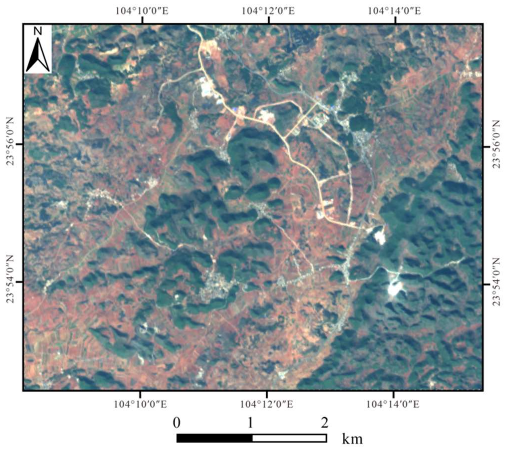
2.1. Study Area

The Chahuazhai gold mining area is located in Qiubei County, Wenshan District, SW China. The scope of the study area is from 104°15′07′′ E to 104°16′23′′ E, 23°57′59′′ N to 23°59′00′′ N. The total area is currently 3.62097 km2.
The study area belongs to the Yangtze Craton block, where the exposed strata include lower Permian and Wujiaping formations of Middle Permian, Yongningzhen formations of Lower Triassic, Ximatang formation of Lower Triassic, and Gejiu formation of Middle Triassic. The lithology consists of mudstone, sandstone, conglomerate, shale, limestone, dolomite, and siliceous rock. Additionally, folds and faults are relatively developed in the area.
The Chahuazhai gold deposit is a typical Carlin-type gold deposit located in the northeast corner of the study area, where the main lithology is siliceous agglomerated limestone, bioclastic limestone, dolomite, and carbonaceous limestone. A fault is developed at the wing of the anticline fold in the mining area. Therefore, the geological background is in favor of Au occurrence (Figure 1).
In this study area, 1:10000 soil sample geochemical data were used with a sampling network of size 100 m ∗ 40 m. For each 100 m ∗ 40 m area, a weighted calculation of the geochemical anomaly values of the four samples formed a combined sample geochemical anomaly value. Then, the field geochemical data processing results have shown that Au geochemical anomalies in the area have a strong correlation with mineralization and spatial characteristics. According to raw soil samples, Au geochemical anomalies in the east of the study area are distributed in a NE trending strip, with a high anomaly value and abundance, especially for the Chahuazhai gold deposit, while Au geochemical anomalies in the west are dominated by two concentration centers and sporadic point anomalies, with relatively low anomaly values (Figure 2).

2.2. Data

2.2.1. Hyperion Data

GaoFen-5 (GF-5) Hyperion data were used as the main remote sensing data in this study. Launched in 2018, the GF-5 satellite operates in a solar synchronous orbit with an average orbital height of 705 km, an inclination of 98.2° and a ground coverage width of 60 km [37]. The visible and shortwave infrared multispectral sensor (VIMS, formerly named multispectral imager) [38] on the GF-5 satellite can obtain 330-band images with spectral intervals of 5 nm (VNIR) and 10 nm (SWIR), and a spectral range from 0.4 to 2.5 μm at a spatial resolution of 30 m. Among the 330 bands, 150 bands are the visible and near-infrared (VNIR) portion with wavelengths from 0.39 to 1.03 μm, 180 bands are the short-wave infrared (SWIR) portion with wavelength from 1.0 to 2.5 μm. The GF-5 image adopted in this study was acquired on 6:11:30, 22 January 2020, by the VIMS. The image has no cloud coverage and is suitable for extracting geoscience information on the earth.

2.2.2. Geochemical Data

A total of 20,144 geochemical samples was used (Figure 3).

2.3. Data Processing

Among the 330 original GF-5 bands, bands No. 193–200 with wavelengths of 1.359–1.418 μm and bands No. 246–262 with wavelengths of 1.805–1.940 μm do not have spectral value (Figure 4 and Figure 5). These 25 bands were removed in the primary stage and the remaining 305 bands were used for further data processing.

Data Preprocessing

First, radiometric calibration and Fast Line-of-sight Atmospheric Analysis of Spectral Hypercubes (FLAASH) atmospheric autocorrection were applied in the GF-5 remote sensing data preprocessing stage. FLAASH is an atmospheric correction method for retrieving spectral reflectance from hyperspectral radiance images by incorporating the MODTRAN radiation transfer model to compensate for atmospheric effects. Then, radiometric calibration calibrates image data to radiance, reflectance, or brightness temperatures.
After applying radiometric calibration and FLAASH to the GF-5 hyperspectral image, the reflection peak around band No. 150 with a wavelength around 1 μm became more evident, which matches the spectral signature of vegetation, as reflection is high in the near infrared wavelength portion (Figure 6 and Figure 7).

Savitzky–Golay Filter

The original remote sensing spectra may contain noises that can result in breakpoints and discontinuity in spectral profile. To improve the continuity of the spectral curve and make the spectral characteristics more obvious, the spectra were then mathematically transformed through a reciprocal logarithm, continuum removal, spectral differentiation, and a Savitzky–Golay filter (S-G filtering).
The S-G filter is a digital filter that can smooth data without distorting the signal tendency. This method is based on convolution by fitting successive subsets of adjacent data points with a low-degree polynomial by the method of linear least squares [39]. Data processed by the S-G filter can better retain spectral characteristics and local features such as bandwidth. Additionally, data processing time can be effectively saved using this method.
R i = j = k k C j R i + j 1 2 k + 1
where R i   is the fitted value, R i + j is the original value of the pixel, C j is the coefficient when the i-th value is filtered, and k is the width of half the filter window.
The result shows that the spectral profile processed by the S-G filter is smoother compared with the radiometric calibration and FLAASH spectral profile. Additionally, the low value around band No. 250 around 1.8 μm was normalized (Figure 8 and Figure 9).

Reciprocal Logarithm

The noise caused by natural light, topography, and other factors can be reduced through the reciprocal logarithm transformation. At the same time, the spectral difference, especially that in the visible light range, can be efficiently enhanced.
R l o g λ i = 1 L o g R λ i
where λ i is the spectral reflectance of the i-th band, R( λ i ) is the spectral reflectance of the corresponding wavelength, and R l o g λ i is the reciprocal of the logarithm of the wavelength λ i .

Continuum Removal

The continuum removal, also known as envelope removal, normalizes reflectance spectra so that individual absorption features from a common baseline can be compared. The connecting lines of the prominent extreme points in the spectrum curve are removed. This method can effectively highlight the absorption characteristics of the spectrum and facilitate the selection of characteristic bands.
  R H λ i = 1 R λ i R C λ i
where λ i is the spectral reflectance of the i-th band, R λ i is the spectral reflectance of the corresponding wavelength, R C λ i is the band reflectance value on the envelope of the band, R λ i R C λ i is the envelope line, and R H λ i is the depth of the band.

First Derivative

The first derivative can make the spectral features in the original spectral curve more obvious. It expands the difference between spectral data and eliminates the influence of the atmosphere and the environment.
  R H λ i = R λ i + 1 R λ i 1 λ i + 1 λ i 1
where λ i + 1 , λ i , λ i 1 are adjacent wavelengths, R λ i + 1 ,   R λ i , R λ i 1 are the spectral reflectances of the corresponding wavelengths, and R H λ i is the first-order differential of the wavelength λ i .

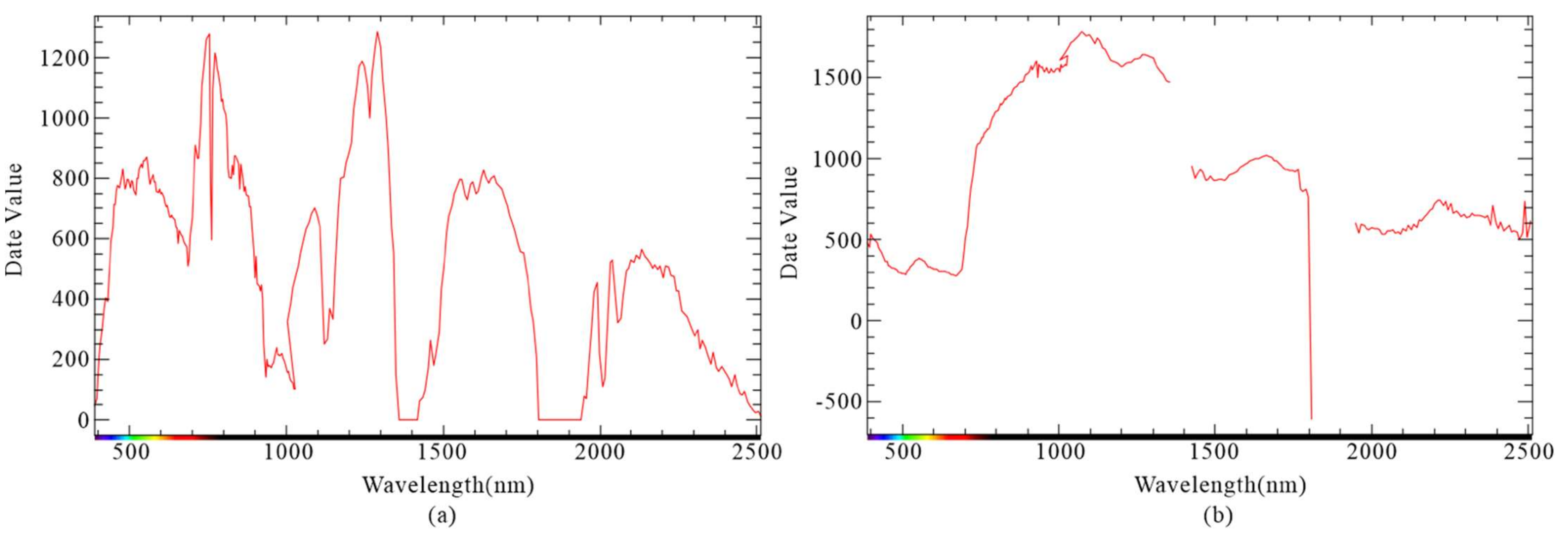
2.4. Characteristic Spectra Selection

By analyzing the relationship between the measured values of Au geochemical anomaly and the spectra of GF-5 data based on correlation analysis, a relatively high correlation band can be selected for modeling.
  R = 1 n 1 i = 1 n X i X ¯ S X Y i Y ¯ S Y
where X and Y are the spectral reflectance at the i-th wavelength and the measured Au content, respectively; X ¯ and Y ¯ are the sample mean of the spectral reflectance and the measured Au content, respectively; S X and S y are the sample variances of the spectral reflectance and the measured Au content, respectively; n is the number of samples; and R is the correlation coefficient.
Based on the correlation analysis, data processed by the Savitzky–Golay (S-G) filter showed the highest correlation between the spectra and Au geochemical anomaly in general among the above methods and the data processed after radiometric calibration and FLAASH (Figure 10). Additionally, breakpoints in the image were removed through the S-G filter. Therefore, the S-G filter processed data were mainly used in further data processing.
The destripe tool was then applied to the image processed by the Savitzky–Golay filter to remove vertical strips in the hyperspectral image. It calculates the mean of every n-th line and normalizes each line to its respective mean when destriping.
Then, Minimum Noise Filter (MNF) transformation was applied. MNF transformation segregates and equalizes the noise in the data and reduces the data dimensionality for target detection by transforming multispectral data to MNF space, smoothing, or rejecting the noisiest components and then re-transforming the data to the original space [40,41] (Figure 11 and Figure 12). The resulting bands of the MNF transformed data are sorted by spatial coherence in descending order. Based on the MNF analysis, the top 17 bands contain most of the information in the image and were used for the IMNF procedure to return back to reflectance space.

2.5. Endmember Choosing

2.5.1. Matched Filtering

Next, the matched filtering technique was applied to the dataset. Matched Filtering (MF), described by Harsanyi and Chang [42] and Boardman et al. [43], finds the abundances of user-defined endmembers using a partial unmixing. This method maximizes the response of a chosen end-member spectrum against that of a composite unknown spectral background.
In this study, due to the lack of the standard spectra of Au geochemical anomalies, the overall spectra processed by MNF, which contains Au geochemical anomaly information, was viewed as the Au geochemical anomaly representing spectra to be matched in the MF process. The Au geochemical anomaly information was extracted by large-sample learning.

2.5.2. Fast Fourier Transform (FFT) with Spectrum-Area (S-A) Method

The FFT forward filter produces an image that shows both the horizontal and vertical spatial frequency components. By applying a filter to the forward FFT data and then performing an inverse transformation, high spatial frequency components, such as noises, can be removed from the image.
The Spectrum–Area (S-A) fractal method was introduced in this study to build the FFT filter for higher accuracy in choosing irregularly distributed endmembers. The S-A method was applied to the FFT transformed spectra and highlighted the anomaly value in the above MF result of GF-5 hyperspectral data. The S-A method can be used to establish power–law relationships between the area with the pixel values greater than s A(≥s) and the pixel value s in the frequency domain after plotting these values on a log–log graph, and the classes separated by the S-A method can show the main types of features on the ground [14]. The horizontally aligned points are considered as the background group, while other points are considered as the anomaly group that is associated with the spatial distribution of mineral occurrences [13]. That is, the number of pixels was applied to approximate the area concept representing “A” and the spectral value representing “S” in the S-A method. Then, statistics were performed on the FFT power image, and log–log values of the number of pixels whose value is greater than and equal to the Digital Number (DN) value against the DN value were plotted.
Based on the plot (Figure 13), the point with the DN value to area value (−7.51629, 87263) and log–log value (−0.876, 4.94083) was chosen as the threshold that separates the background and the geochemical anomaly. Through this FFT filter, pixels whose logarithm value of the DN value is less than −7.51629 were filtered out. Finally, this filter created using the S-A method was applied in the FFT domain and then inverted back to the original space domain. In this way, Au geochemical element anomalies information was obtained.

2.6. Regression Models

Several regression models, including Multiple Linear Regression (MLR), Partial Least Squares (PLS) regression, BP neural network and Geographically Weighted Regression (GWR), were used in this study to reveal the coupling relationship between GF-5 spectra and Au content. For multiple linear regression, partial least squares regression and BP neural network, values of bands Nos. 239, 240, 246, 294, and 305 of the GF-5 hyperspectral data processed by the Savitzky–Golay (S-G) filter were chosen as the independent variables, since spectra values of the above bands have the highest correlation coefficients with the Au content.

2.6.1. Multiple Linear Regression (MLR)

Multiple linear regression analysis establishes regression equations between multiple independent variables and dependent variables to predict values of dependent variables. Compared with the traditional unary regression analysis, it has higher accuracy.
Y = β 0 + β 1 X 1 + + β j X j + + β n X n + ε
where Y is the dependent variable (Au content), X n is the n-th independent variable (GF-5 spectra value), and β n is the regression coefficient of the n-th independent variable.

2.6.2. Partial Least Squares (PLS) Regression

Partial least squares regression is a statistical method that is related to principal component regression. It projects predictor variables and observed variables into a new space to find a linear regression model. In this study, four PLS components are used to build the final PLS regression model.
  X = T P T + E
Y = U Q T + F
where X is a matrix of predictors (Au content), and Y is a matrix of responses (GF-5 spectra value); T and U are, respectively, projections of X and projections of Y; P and Q are orthogonal loading matrices; and matrices E and F are the error terms. The decompositions of X and Y are made so as to maximize the covariance between T and U.

2.6.3. Back Propagation (BP) Neural Network

The Back Propagation (BP) network algorithm is a widely applied multi-layer feedforward network trained according to the error back propagation algorithm. In this case, a BP neural network with one input layer (GF-5 spectra value), one output layer (Au content), and three hidden layers was built. Each hidden layer had ten neurons.
The activation function for the first two hidden layers is the positive linear transfer function, and the neural transfer function was used for the last hidden layer. For the performance function, the mean squared error function was chosen.
The coding for the BP neural network was done by MATLAB. The maximum number of epochs to train this network was set to 100, and the learning rate was set to 0.1. The maximum number of validation checks was set to 6 and the performance goal was set to 0.00004. Among the 20,144 sample points, 18,144 points were used for training, and the other 2000 points were used for testing.

2.6.4. Geographically Weighted Regression (GWR)

Geographically Weighted Regression (GWR) calibrates a separate regression model at each location through a data-borrowing scheme in which distance-weights observations from each location serve as regression points. A GWR model may be specified as:
y i = β i 0 + k = 1 p β i k x i k + ε i , i = 1 , , n
where y i is the dependent variable at location i   , β i 0 is the intercept coefficient at location i , x i k is the k-th explanatory variable at location i , β i k is the k-th local regression coefficient for the k-th explanatory variable at location i , and εi is the random error term associated with location i . i is typically indexed by two-dimensional geographic coordinates ( u i , v i ), indicating the location of the regression point [44,45].
Data after inverse FFT transformation were loaded for further processing and their corresponding values were assigned to points in the shapefile of the sampling area. The GF-5 spectra values were set as the independent variables, and the Au geochemical anomaly was set as the dependent variable. X and Y coordinates were also used in the GWR model. A Gaussian model type was chosen as the Kernel type. A Gaussian kernel option (local weighting scheme), a number of neighbors (bandwidth) neighbor type, and the golden search neighborhood selection method (distance and number of neighbors) were chosen (Table 1).
It should be noted that the prediction locations should be within the 30% extended boundary box of the input features, since predictions are only reliable in the same area where the model is estimated for geographically weighted regression.

3. Results

Among the above four methods, multiple linear regression, partial least squares regression and BP neural network showed poor performance in finding the regression model between the selected spectra of the GF-5 data and the field-measured Au content, with R 2 or accuracies of 0.004, 0.4037, and 0.22799, respectively. The root-mean-square deviation (RMSE) values of multiple linear regression and partial least squares regression were 3.005 and 7.793053, respectively. After applying endmember choosing methods to the GF-5 hyperspectral data, the GWR model showed high R 2 and low RMSE between the raster value of points of the GF-5 image processed after inverse FFT and Au content. R 2 was 0.6133 and RMSE was 0.3038 for the GWR model, which are much higher R 2 and much lower RMSE values compared to those of the multiple linear regression, partial least squares regression and BP neural network models (Table 2 and Table 3).
In general, the GWR prediction result, where points are generated on a point per pixel base from each pixel of the remote sensing image, is consistent with the field-measured geochemical anomaly values. Specifically, in the east of the study area, predicted Au geochemical anomalies are distributed in a NE trending strip, with a high anomaly value and large abundance, whereas in the west of the study area, predicted Au geochemical anomalies are with relatively low anomaly values, dominated by two concentration centers and sporadic point anomalies (Figure 14).
According to the field work results, the geochemical anomaly values of the field soil samples at No. 1, 2, 3 are 368 ppb, 308 ppb, and 24 ppb, respectively. The trend of the field data is generally consistent with the trend of the prediction results (Figure 15).

4. Discussions

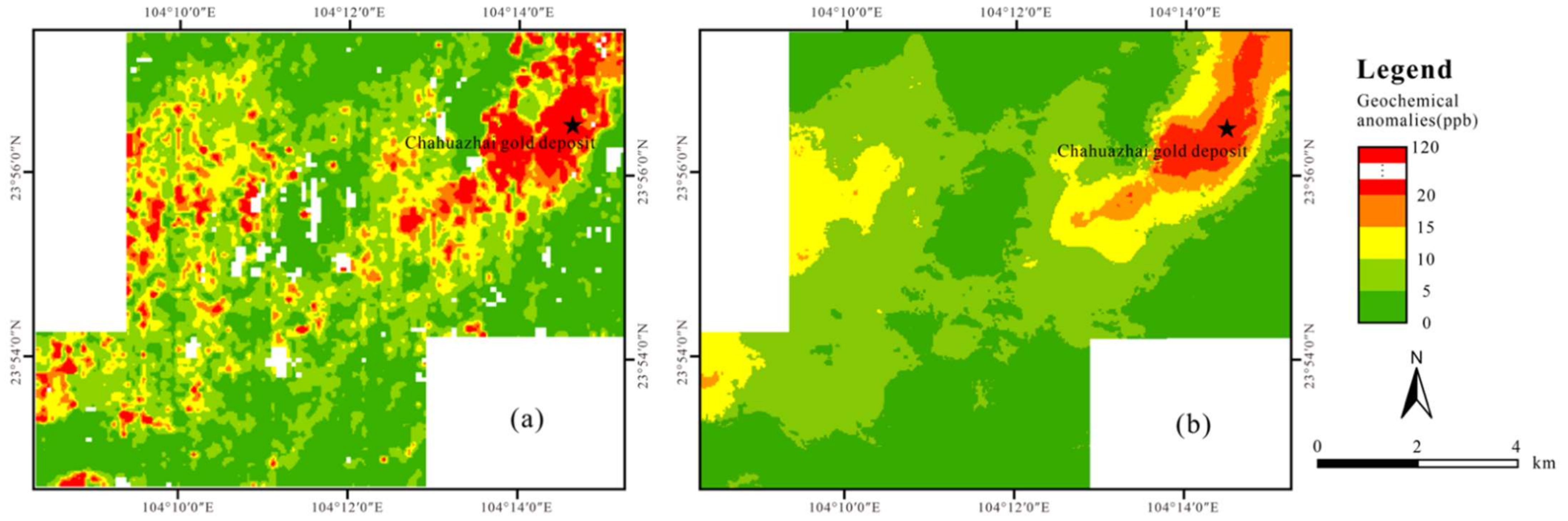
4.1. Prediction Results Spatial Distribution

In general, the trend of the prediction results of Au geochemical anomalies matched that of the field geochemical exploration samplings (Figure 16). The trend of the prediction results in the east of the study area generally matched that of the measured sampling values. However, values of some points in the west of the study area were not well predicted. Moreover, though the red color is used to represent points with Au geochemical anomaly values between 20 and 120 for both the geochemical exploration results and GWR prediction results, the highest value in the geochemical exploration sampling results reached 120 whereas the highest value for the prediction results was only around 47.
Particularly, the GWR model tends to normalize the dependent values. The general distribution trend of the field-measured geochemical anomaly exploration content is preserved but the extreme geochemical anomaly values are not very well predicted. While GWR can predict the general trend of the geochemical anomaly data well, it may not be ideal for predicting extreme geochemical anomaly values.

4.2. Influence Factors of Prediction

4.2.1. Lithology and Tectonic

There are differences in the fitting accuracy of different areas, and lithology may contribute to the differences. The exposed strata in the east of the study area mainly consist of a middle Permian Wujiaping formation, Lower Permian, Quaternary Pleistocene alluvium and Quaternary Pleistocene pulluvial alluvium. The lithology of this formation mainly consists of limestone, and limestone-related alluvium (Figure 17).
The exposed strata in the west of the study area are mainly the first member of the Gejiu formation of Middle Triassic, pulluvial alluvium of Quaternary Pleistocene and alluvial accumulation of Quaternary Pleistocene. The lithology of this area mainly consists of dolomite, limestone, and carbonate-related alluvium with sandy gravel clay. There are scattered high Au predicted geochemical anomaly concentrations in two zones in the west: One in the zone with relatively developed faults in the northwest part of the study area, and the other in the first member of Gejiu formation with the alluvium of Quaternary Pleistocene in the southwest part of the study area. In addition, the southwest part of the study area is largely covered by Quaternary Pleistocene pulluvial alluvium with gravel clay related to carbonate with a low Au geochemical anomaly.
Carlin-type gold deposits in the Chahuazhai area, where Devonian and Permian are the main ore-bearing strata, are strongly impacted by geological structures, including the Qiubei anticline, NNW-trending faults, and fractures. These tectonics provided mineral fluid migration channels. The intersection of the Qiubei anticline and the NNW-trending structure, as well as the fissures that promoted ore mineralization enrichment, provided good geological conditions for the formation of gold deposits. The prediction result trend is consistent with the tectonics, especially the anticline extension direction and the distribution of favorable tectonic combination areas.
In conclusion, the overall Au geochemical anomaly prediction results are consistent with the field-measured Au geochemical exploration results, which are closely related to the lithology of the study area. Au geochemical anomaly results were not well predicted in carbonate or carbonated-related alluvium in either the west or the east of the study area. Moreover, favorable tectonic assemblage, especially anticline, also plays an important role in geochemical anomaly enrichment in the prediction result.

4.2.2. Vegetation

Besides lithology, vegetation coverage may also have a significant impact on the prediction fitting results of Au geochemical anomalies in this area.
According to the geochemical exploration result, high Au geochemical anomaly values are in the area where vegetation is sparse (Figure 18). In particular, high Au anomalies are distributed in zone A in a northeastern trend strip, in the west part of zone B, and in most parts of the southwestern part of zone C. Additionally, some high Au anomalies are sparsely distributed in zone D. In the view of the original GF-5 hyperspectral image, vegetation is sparsely distributed in zones A, B, and C. By contrast, vegetation is densely distributed in zone D.
While prediction of Au geochemical anomaly distribution trends in study zones A, B, and C generally matches that of the measured values, values of some points in zone D are not well predicted. For zone D, some Au geochemical exploration values are greater than 20 (shown in red color), but these values were not predicted through the GWR model. Therefore, it is reasonable to assume that vegetation coverage may have a significant impact on the fitting of Au geochemical values; however, their internal relationship is still unclear. The way that vegetation coverage affects the mechanism of geochemical anomalies fitting still needs to be further analyzed and studied.

5. Conclusions

This study demonstrated an efficient way to obtain Au geochemical anomalies with GF-5 data. The study showed that hyperspectral data are not only able to identify the rocks associated with Au mineralization and characterize the mineralogy and mineral chemistry of complex minerals, but can also be applied to extract Au geochemical anomalies, which are a strong indicator of gold mineralization, especially Carlin-type gold deposit. This paper implies that the S-G filter, S-A method, and MF are capable of extracting Au geochemical anomaly endmember information from GF-5 hyperspectral data. The above methods can be used for effectively separating background values and obtaining Au geochemical anomaly values from the GF-5 hyperspectral data. In particular, MF with large-sample learning provides a fast and innovative endmember finding method, which can be more accurate for choosing Au geochemical anomaly-containing endmembers than common traditional filters. Such a finding is helpful for the analysis of geochemical anomalies in the mining area and provides a useful tool for the indication of ore or near ore.
This study also found a method for predicting Au geochemical anomaly based on the GF-5 hyperspectral data and an understanding of the GF-5 spectra response mechanism. This study demonstrated that the coupling relationship between the Au content in the Chahuazhai gold deposit and the spectra of the processed GF-5 hyperspectral data is closely related to local geographical attributes. At the same time, the GWR model was used to reveal the spectra response mechanism of GF-5 data to the field Au geochemical anomalies. Many geochemical sampling efforts may be saved, and ore prospecting can be more efficient.
Vegetation, lithology, and tectonics may be important factors that impact the prediction results of the GWR model between hyperspectral data and Au geochemical anomaly values. According to the above analysis, high Au geochemical anomaly values are closely associated with sparse vegetation coverage, carbonate-related rocks of the Permian Strata and Quaternary alluvium, and the Qiubei NE-trending anticline. It should be noted that the geographically weighted regression model can only provide reliable prediction in a 30% extended area of the input area for local geographic attributes. The mechanism of the impact of vegetation and lithology on the prediction of the Au geochemical anomaly from GF-5 data needs to be further studied.

Author Contributions

Conceptualization, Z.Z. and Y.Q.; Methodology, Y.Q., Software, Y.Q., X.Z. and Z.L.; Formal Analysis, Y.Q., Resources, C.Y.; Data Curation, Y.Q., X.Z. and Z.L.; Writing—Original Draft Preparation, Y.Q.; Writing Review and Editing, Z.Z. and Q.H.; Funding Acquisition, Z.Z. All authors have read and agreed to the published version of the manuscript.

Funding

This study was funded by the National Natural Science Foundation of China (Grant No.41462015, 41872251 and 42061038), the Joint Fund of Science Technology Department of Yunnan Province and Yunnan University (Grant No.2018FY001(-019)), and the entrusted project of the Second Geological Brigade of Yunnan Bureau of Geology and Mineral Exploration and Development (Grant No. K207005210032). Research on the metallogenic regularity of shallow-form low-temperature hydrothermal deposits in southeastern Yunnan and prediction of prospecting target areas-remote sensing geological interpretation (Grant No. K207005210032).

Institutional Review Board Statement

Not applicable.

Informed Consent Statement

Not applicable.

Data Availability Statement

The data presented in this study are available upon request from the corresponding author.

Acknowledgments

The authors would like to thank the anonymous reviewers for providing valuable feedback on the manuscript.

Conflicts of Interest

The authors declare no conflict of interest.

References

  1. Chen, S.; Hu, G.; Zhou, Z. Geo-anomaly structure and mineral prediction in the Mianxian–Lueyang–Ningqiang area. Earth Sci. J. China Univ. Geosci. 1999, 24, 472–475. [Google Scholar]
  2. Yuan, Y.; Li, S.; Peng, J.; Si, J.; Cheng, H.; Sun, J.; Wei, J.; Shao, J. An integrated ore prospecting model for the Nyasirori gold deposit in Tanzania. Geol. China 2019, 2, 407–421. [Google Scholar] [CrossRef]
  3. Liu, H.; Beaudoin, G. Geochemical signatures in native gold derived from Au-bearing ore deposits. Ore Geol. Rev. 2021. [Google Scholar] [CrossRef]
  4. Zhao, J.; Chen, S.; Zuo, R. Identifying geochemical anomalies associated with Au–Cu mineralization using multifractal and artificial neural network models in the Ningqiang district, Shaanxi, China. Geochem. Explor. 2016, 164, 54–64. [Google Scholar] [CrossRef]
  5. Sun, X.; Zheng, Y.; Wang, C.; Zhao, Z.; Gneg, X. Identifying geochemical anomalies associated with Sb–Au–Pb–Zn–Ag mineralization in North Himalaya, southern Tibet. Ore Geol. Rev. 2016, 73, 1–12. [Google Scholar] [CrossRef]
  6. Simon, G.; Kesler, S.; Chryssoulis, S. Geochemistry and textures of gold-bearing arsenian pyrite, Twin Creeks, Nevada: Implications for deposition of gold in Carlin-type deposits. Econ. Geol. 1999, 94, 405–421. [Google Scholar] [CrossRef]
  7. Li, Z. Comparative Geology and Geochemistry of Sedimentary Rock-Hosted (Carlin-Type) Gold Deposits in the People’s Republic of China and in Nevada, United States of America; Order No. 1395247; University of Nevada: Reno, NV, USA, 1999. [Google Scholar]
  8. Hu, Z.; Su, C.; Bi, W.; Tu, Z.; Hofstra, H. Geology and geochemistry of Carlin-type gold deposits in China. Miner. Deposita. 2002, 37, 378–392. [Google Scholar] [CrossRef]
  9. Zhang, C.; Spiro, B.; Halls, C.; Stanley, J.; Yang, Y. Sediment-hosted disseminated gold deposits in Southwest Guizhou, PRC: Their geological setting and origin in relation to mineralogical, fluid inclusion, and stable-isotope characteristics. Int. Geol. Rev. 2003, 45, 407–470. [Google Scholar] [CrossRef]
  10. Peters, G.; Huang, J.; Li, Z.; Jing, C. Sedimentary rock-hosted Au deposits of the Dian-Qian-Gui area, Guizhou, and Yunnan Provinces, and Guangxi District, China. Ore Geol. Rev. 2007, 31, 170–204. [Google Scholar] [CrossRef]
  11. Su, C.; Heinrich, A.; Pettke, T.; Zhang, C.; Hu, Z.; Xia, B. Sediment-hosted gold deposits in Guizhou, China: Products of wall-rock sulfidation by deep crustal fluids. Econ. Geol. 2009, 104, 73–93. [Google Scholar] [CrossRef] [Green Version]
  12. Hofstra, A.H.; Leventhal, J.S.; Northrop, R.; Landis, G.P.; Rye, R.O.; Birak, D.J.; Dahl, A.R. Genesis of sediment-hosted disseminated-gold deposits by fluid mixing and sulfidization: Chemical-reaction-path modeling of ore-depositional processes documented in the Jerritt Canyon district, Nevada. Geology 1991, 19, 36–40. [Google Scholar] [CrossRef]
  13. Su, W.; Dong, W.; Zhang, X.; Shen, N.; Hu, R.; Hofstra, A.; Cheng, L.; Xia, Y.; Yang, K. Carlin-Type gold deposits in the Dian-Qian-Gui “Golden Triangle” of Southwest China. Diversity in Carlin-Style Gold Deposits. Rev. Econ. Geol. 2018, 20, 157–185. [Google Scholar]
  14. Su, W.C.; Hu, R.Z.; Xia, B.; Xia, Y.; Liu, Y.P. Calcite Sm-Nd isochron age of the Shuiyindong Carlin-type gold deposit, Guizhou, China. Chem. Geol. 2009, 258, 269–274. [Google Scholar] [CrossRef]
  15. Cline, J.S.; Muntean, J.L.; Gu, X.X.; Xia, Y. A comparison of Carlin-type gold deposits: Guizhou Province, Golden Triangle, Southwest China, and Northern Nevada, USA. Earth Sci. Front. 2013, 20, 1–18. [Google Scholar]
  16. Reich, M.; Kesler, S.E.; Utsunomiya, S.; Palenik, C.S.; Chryssoulis, S.L.; Ewing, R.C. Solubility of gold in arsenian pyrite. Geochim. Et Cosmochim. Acta 2005, 69, 2781–2796. [Google Scholar] [CrossRef]
  17. Gopon, P.; Douglas, J.O.; Auger, M.A.; Hansen, L.; Wade, J.; Cline, J.S.; Robb, L.J.; Moody, M.P. A Nanoscale Investigation of Carlin-Type Gold Deposits: An Atom-Scale Elemental and Isotopic Perspective. Econ. Geol. 2019, 114, 1123–1133. [Google Scholar] [CrossRef] [Green Version]
  18. Zuo, R.; Wang, J.; Xiong, Y.; Wang, Z. The processing methods of geochemical exploration data: Past, present, and future. Appl. Geochem. 2021, 132, 105072. [Google Scholar] [CrossRef]
  19. Cheng, Q.; Agterberg, F.P.; Bonham-Carter, G.F. A spatial analysis method for geochemical anomaly separation. Geochem Explor. 1996, 56, 183–195. [Google Scholar] [CrossRef]
  20. Cheng, Q. Multifractality and spatial statistics. Comput. Geosci. 1999, 25, 949–961. [Google Scholar] [CrossRef]
  21. Ayoobi, I.; Tangestani, M.H. Evaluation of subpixel unmixing algorithms in mapping the porphyry copper alterations using EO-1 Hyperion data, a case study from SE Iran. Remote Sens. Appl. Soc. Environ. 2018, 10, 120–127. [Google Scholar] [CrossRef]
  22. van der Meer, F.; Vazquez-Torres, M.; van Dijk, P.M. Spectral characterization of ophiolite lithologies in the troodos ophiolite complex of Cyprus and its potential in prospecting for massive sulphide deposits. Int. J. Rem. Sens. 1997, 18, 1245–1257. [Google Scholar] [CrossRef]
  23. Wan, Y.; Fan, Y.; Jin, M. Application of hyperspectral remote sensing for supplementary investigation of polymetallic deposits in Huaniushan ore region, northwestern China. Sci. Rep. 2021, 11, 440. [Google Scholar] [CrossRef] [PubMed]
  24. Ye, B.; Tian, S.; Cheng, Q.; Ge, Y. Application of lithological mapping based on Advanced Hyperspectral Imager (AHSI) imagery onboard Gaofen-5 (GF-5) satellite. Remote Sens. 2020, 12, 3990. [Google Scholar] [CrossRef]
  25. Liu, L.; Shang, K. Mineral information extraction based on Gaofen-5’s thermal infrared data. ISPRS. 2018, 42, 1157–1160. [Google Scholar] [CrossRef] [Green Version]
  26. Cracknell, M.J.; Reading, A.M. Geological mapping using remote sensing data: A comparison of five machine learning algorithms, their response to variations in the spatial distribution of training data and the use of explicit spatial information. Comput. Geosci. 2014, 63, 22–33. [Google Scholar] [CrossRef] [Green Version]
  27. Othman, A.; Gloaguen, R. Improving lithological mapping by SVM classification of spectral and morphological features: The discovery of a new chromite body in the Mawat ophiolite complex (Kurdistan, NE Iraq). Remote Sens. 2014, 6, 6867–6896. [Google Scholar] [CrossRef] [Green Version]
  28. Othman, A.A.; Gloaguen, R. Integration of spectral, spatial and morphometric data into lithological mapping: A comparison of different Machine Learning Algorithms in the Kurdistan Region, NE Iraq. J. Asian Earth Sci. 2017, 146, 90–102. [Google Scholar] [CrossRef]
  29. Lary, D.J.; Alavi, A.H.; Gandomi, A.H.; Walker, A.L. Machine learning in geosciences and remote sensing. Geosci. Front. 2016, 7, 3–10. [Google Scholar] [CrossRef] [Green Version]
  30. Wei, J.; Liu, X.; Liu, J. Integrating textural and spectral features to classify silicate- bearing rocks using Landsat 8 data. Appl. Sci. 2016, 6, 283. [Google Scholar] [CrossRef] [Green Version]
  31. Pourmohammadi, P.; Strager, M.P.; Dougherty, M.J.; Adjeroh, D.A. Analysis of land development drivers using Geographically Weighted Ridge Regression. Remote. Sens. 2021, 13, 1307. [Google Scholar] [CrossRef]
  32. Shabrina, Z.; Buyuklieva, B.; Ng, M.K.M. Short-term rental platform in the urban tourism context: A Geographically Weighted Regression (GWR) and a Multiscale GWR (MGWR) approaches. Geogr. Anal. 2021, 53, 686–707. [Google Scholar] [CrossRef]
  33. Liu, C.; Wu, X.; Wang, L. Analysis on land ecological security change and affect factors using RS and GWR in the Danjiangkou Reservoir area, China. Appl Geogr. 2019, 105, 1–14. [Google Scholar] [CrossRef]
  34. Kumar, C.; Chatterjee, S.; Oommen, T.; Guha, A. Automated lithological mapping by integrating spectral enhancement techniques and machine learning algorithms using AVIRIS-NG hyperspectral data in Gold-bearing granite-greenstone rocks in Hutti, India. Int. J. Appl. Earth Obs. 2020, 86, 102006. [Google Scholar] [CrossRef]
  35. Pour, A.B.; Hashim, M.; van Genderen, J. Detection of hydrothermal alteration zones in a tropical region using satellite remote sensing data: Bau goldfield, Sarawak, Malaysia. Ore Geol. Rev. 2013, 54, 181–196. [Google Scholar] [CrossRef]
  36. Lypaczewski, P.; Rivard, B.; Gaillard, N.; Perrouty, S.; Lauzière, N.P.; Bérubé, C.L.; Linnen, R.L. Using hyperspectral imaging to vector towards mineralization at the Canadian Malartic gold deposit, Québec, Canada. Ore Geol. Rev. 2019, 111, 102945. [Google Scholar] [CrossRef]
  37. Ye, X.; Ren, H.; Liu, R.; Qin, Q.; Liu, Y.; Dong, J. Land surface temperature estimate from Chinese Gaofen-5 satellite data using split-window algorithm. IEEE Trans. Geosci. Remote Sens. 2017, 55, 5877–5888. [Google Scholar] [CrossRef]
  38. Ren, H.; Ye, X.; Liu, R.; Dong, J.; Qin, Q. Improving land surface temperature and emissivity retrieval from the Chinese Gaofen-5 satellite using a hybrid algorithm. IEEE Trans. Geosci. Remote Sens. 2018, 56, 1080–1090. [Google Scholar] [CrossRef]
  39. Savitzky, A.; Golay, M.J.E. Smoothing and differentiation of data by simplified least squares procedures. Anal. Chem. 1964, 36, 1627–1639. [Google Scholar] [CrossRef]
  40. Boardman, J.W.; Kruse, F.A. Automated spectral analysis: A geological example using AVIRIS data, north Grapevine Mountains, Nevada: In Proceedings, ERIM Tenth Thematic Conference on Geologic Remote Sensing; Environmental Research Institute of Michigan: Ann Arbor, MI, USA, 1994. [Google Scholar]
  41. Green, A.A.; Berman, M.; Switzer, P.; Craig, M.D. A transformation for ordering multispectral data in terms of image quality with implications for noise removal. IEEE Trans. Geosci. Remote Sens. 1988, 26, 65–74. [Google Scholar] [CrossRef] [Green Version]
  42. Harsanyi, J.C.; Chang, C.I. Hyperspectral image classification and dimensionality reduction: An orthogonal subspace projection approach. IEEE Trans. Geosci. Remote Sens. 1994, 32, 779–785. [Google Scholar] [CrossRef] [Green Version]
  43. Boardman, J.W. Leveraging the high dimensionality of AVIRIS data for improved sub-pixel target unmixing and rejection of false positives: Mixture tuned matched filtering. In Summaries of the Seventh Annual JPL Airborne Geoscience Workshop; JPL Publication: Pasadena, CA, USA, 1998; Volume 6. [Google Scholar]
  44. Tobler, W.R. A Computer movie simulating urban growth in the Detroit Region. Econ. Geogr. 1970, 46, 234. [Google Scholar] [CrossRef]
  45. Fotheringham, A.S.; Brunsdon, C.; Charlton, M. Geographically Weighted Regression: The Analysis of Spatially Varying Relationships; John Wiley & Sons: Hoboken, NJ, USA, 2002. [Google Scholar]
Figure 1. Geological map of Chahuazhai gold mining area. 1. Geological boundary; 2. Fault; 3. Quaternary Pleistocene alluvium; 4. Quaternary Pleistocene flood alluvium; 5. Third member of Gejiu formation of Middle Triassic; 6. Second member of Gejiu formation of Middle Triassic; 7. First member of Gejiu formation of Middle Triassic; 8. Yongningzhen formation of Lower Triassic; 9. Ximatang formation of Lower Triassic; 10. Wujiaping formation of Middle Permian; 11. Lower Permian.
Remotesensing 14 00109 g001
Figure 2. Au anomalies from samples in the study area.
Remotesensing 14 00109 g002
Figure 3. Au geochemical soil samples distributions.
Remotesensing 14 00109 g003
Figure 4. Raw GF-5 spectral profile.
Remotesensing 14 00109 g004
Figure 5. Original GF-5 hyperspectral image.
Remotesensing 14 00109 g005
Figure 6. (a) Raw GF-5 spectral profile; (b): GF-5 spectral profile after radiometric calibration and FLAASH.
Remotesensing 14 00109 g006
Figure 7. (a) Raw GF-5 hyperspectral image; (b) GF-5 image processed by radiometric calibration and FLAASH.
Remotesensing 14 00109 g007
Figure 8. (a) Spectral profile after radiometric calibration and FLAASH; (b) spectral profile after S-G filter.
Remotesensing 14 00109 g008
Figure 9. (a) Image processed by radiometric calibration and FLAASH; (b) image processed by the S-G filter.
Remotesensing 14 00109 g009
Figure 10. Correlation analysis results between spectra and Au measured content for preprocessed results.
Remotesensing 14 00109 g010
Figure 11. MNF analysis curve.
Remotesensing 14 00109 g011
Figure 12. (a) Image before MNF transformation; (b) image after MNF transformation.
Remotesensing 14 00109 g012
Figure 13. Log–log plot of spectrum-area value for MF result.
Remotesensing 14 00109 g013
Figure 14. GWR prediction results of geochemical anomalies.
Remotesensing 14 00109 g014
Figure 15. Testing field soil sample locations.
Remotesensing 14 00109 g015
Figure 16. (a) Geochemical exploration sampling results; (b) GWR prediction results.
Remotesensing 14 00109 g016
Figure 17. (a) Geological background of the study area: 1. Chahuazhai gold deposit; 2. Geological boundary; 3. Fault; 4. Quaternary Pleistocene alluvium; 5. Quaternary Pleistocene pulluvial alluvium; 6. Third member of Gejiu formation of Middle Triassic; 7. Second member of Gejiu formation of Middle Triassic; 8. First member of Gejiu formation of Middle Triassic; 9. Yongningzhen formation of Lower Triassic; 10. Ximatang formation of Lower Triassic; 11. Wujiaping formation of Middle Permian; 12. Lower Permian. (b) GWR prediction results. (c) Geochemical exploration results.
Remotesensing 14 00109 g017
Figure 18. Zones of interest. (a) Original GF-5 hyperspectral image; (b) GWR prediction results; (c) geochemical exploration results.
Remotesensing 14 00109 g018
Table 1. GWR model parameters.
Model Type Neighborhood TypeNeighborhood Selection Type Local Weighting Scheme
GaussianNumber of neighborsGolden searchGaussian
Table 2. Comparison of Multiple Linear Regression (MLR), Partial Least Squares (PLS) regression and Geographically Weighted Regression (GWR) for analysis of GF-5 data and field-measured Au content.
Multiple Linear RegressionPartial Least Squares RegressionGeographically Weighted Regression
R20.0040.40990.6295
Adjusted R20.0040.40370.6133
RMSE3.0057.9030530.3038
Table 3. BP neural network result.
AccuracyBP Neural Network
Training0.23424
Validation0.20639
Test0.21792
Total0.22799
Publisher’s Note: MDPI stays neutral with regard to jurisdictional claims in published maps and institutional affiliations.

