Article

From 1/4° to 1/8°: Influence of Spatial Resolution on Eddy Detection Using Altimeter Data

1
College of Marine Technology, Institute for Advanced Ocean Study, Ocean University of China, Qingdao 266100, China
2
Qingdao National Laboratory for Marine Science and Technology, Qingdao 266237, China
*
Author to whom correspondence should be addressed.
Remote Sens. 2022, 14(1), 149; https://doi.org/10.3390/rs14010149
Submission received: 2 November 2021 / Revised: 26 December 2021 / Accepted: 26 December 2021 / Published: 30 December 2021
(This article belongs to the Section Ocean Remote Sensing)

Abstract

:
A substantial portion of ocean eddies, especially small ones, may be missed due to insufficient spatial or temporal sampling by satellite altimetry. In order to illustrate the influence of spatial resolution on eddy detection, this study provides a comparison of eddy identification, tracking, and analysis between two sets of merged altimeter data with spatial resolutions of 1/4° and 1/8°. One main study area (the Mediterranean Sea), and three confirmatory areas (the South-China Sea, the North-West Pacific, and the South-East Pacific) are chosen. The results show that the number and density of eddies captured by the 1/8° data are about twice as much as those captured by the 1/4° data, while the ratios of corresponding eddy parameters, i.e., radius, amplitude, (eddy kinetic energy (EKE)) are about 0.6–0.8 (1.3) for the two datasets (1/8° ÷ 1/4°). Long-term eddy tracking (1993–2018) is conducted in the Mediterranean Sea, indicating that the improvement in spatial resolution will increase the observed values of both the lifetime and the propagation distance of robust eddies. The number of eddies identified using the 1/4° data only accounts for ~30% to 60% of those identified using the 1/8° data. However, for eddies that can be detected using the two datasets, ~5% to 10% present errors (i.e., confusion). In comparison between the four regions, we find that for the enclosed seas with complex conditions, the increase in spatial resolution may lead to more significant improvements in the efficiency and accuracy of eddy detection.

Graphical Abstract

1. Introduction

Ocean eddy is a general term for the rotational motion of seawater with a scale smaller than a Rossby wave, which is controlled by the (quasi) geostrophic potential vorticity conservation equation [1]. They are broadly distributed in the ocean and play a significant role in the transportation and mixing of physical and biological properties [1,2,3]. As a ubiquitous ocean phenomenon, ocean eddies account for ~90% of the kinetic energy of the global ocean [4]. The momentum transport resulting from them has effectively impacted many features of the circulation, large-scale seawater distribution, and ecosystem characteristics of the global ocean [5,6,7,8,9,10,11]. Eddies can enhance biological production by increasing the concentration of nutrients in the open ocean, which has an important impact on the distribution of marine primary productivity [12,13]. Moreover, due to the large space and time scale span of eddies, they can also interact with the atmosphere through processes including wind stress, cloud cover, heat fluxes, and precipitations, resulting in energy transmission between ocean and atmosphere. Ocean eddies are also responsible for energy conversion between different scale phenomena in the ocean [14,15]. As a result, the study of ocean eddies has become a core theme of modern oceanography over the past few decades [16].
The detection of ocean eddies using remote sensing observations has focused on ocean properties such as sea surface temperature (SST), sea surface ocean color (chlorophyll concentration), sea surface wind (SSW), and sea surface height (SSH) [17,18]. D’Alimonte [19] used SST data to iterate SST isotherms for automatic eddy identification and correlation structure characterization. Dong et al. [20] proposed an automated approach to detect ocean eddies from SST data. Gonzalez-Silvera et al. [21] effectively identified and tracked 18 eddies in the tropical Pacific Ocean using five months data from SeaWiFS and AVHRR sensors. Park et al. [22] made an observation of diurnal variations in eddy sea-surface currents using GOCI data.
However, constrained by atmospheric processes such as clouds and some ocean phenomena, eddy detection using such ocean properties is prone to false positives [23]. Carsy et al. [24] detected eddies in southern Greenland using SAR images of sea ice in the winter of 1992. Rouault et al. [25] identified and studied several eddies near the Agulhas Current using Envisat images. Although SAR-based eddy detection has a high spatial resolution that can capture small-scale eddies, it is vulnerable to the influence of the SSW field. Eddy identification with profiling Argo floats has made great progress [26], yet it is more specific to the vertical structure of eddies.
Since the early 1980s, it has been recognized that eddy variability scales are particularly accessible to capture by altimeter [27]. It is worth noting that the motion of mesoscale eddies may lead to the rise or fall of continuously closed quasi-circular sea level contours, that is, the surface geometric representation of eddies that allows them to be identified effectively by satellite altimetry [12]. In the past few years, satellite altimetry technology has greatly improved our understanding of large-scale ocean circulation and its interaction with mesoscale dynamics, and has been effectively applied to the tracking systems of ocean eddies on regional or global scales, leading to the formation of several decadal eddy datasets with a grid size of 1/4° on daily or weekly repetitions [12,28].
In the wake of the combination of these unprecedented measurements with other parallel multidisciplinary data sources, a significant process has been made in many fields of marine science [29,30]. However, the existing satellite altimeters are still insufficient in horizontal resolution and vertical profile detection abilities. The measurement process, and associated mapping programs used to calculate the gridded maps, can distort the features of an eddy field to a large extent. There is an along-track/cross-track inequality in the sampling interval of the current generation of satellite altimeters. This inherent spatial or temporal heterogeneity leads to little sampling in the meridional/zonal dimensions, and the resulting sampling field tends to mix the unresolved scales into larger ones and hence overestimating the number of large eddies and strongly modifying the amplitude of eddies. More importantly, eddy detection methods based on SSH gridded products with low-resolution largely underestimate the density of eddies, capturing only ~6% to 16% of the number of real eddies [31]. Most of the small-scale eddies with radius scales of 10–50 km are missed.
According to Chelton et al. [1], the feature scale that can be resolved by AVISO merged altimeter data is around 0.4°, which is approximately ~44.4 km at the equator and ~31.4 km at the middle latitudes. By removing the sensor noise, the scale improved to 25–35 km by 2012 [32]. More recently, the emergence of more altimeter satellites has further improved the feature scale to approximately 20 km [33]. Previous work has assessed the effects of data resolution on eddy research. For example, the eddy contribution to the meridional transport of salt in the North Atlantic was studied using the 1/4° and 1/12° resolution data [34]. The eddies in the Mediterranean Sea were studied by using 1/8° data and higher resolution model data such as 1/32°, 1/36° and 1/120° [35,36,37]. While the eddy properties detected by the model datasets at higher resolutions are expected (i.e., more quantity, smaller radius, and longer life), they are artificially improved “false” accuracy and have no practical significance. Therefore, comparisons of the ocean eddy detection ability of 1/4° and 1/8° resolution altimeter data are essential for marine science. The upcoming Surface Water and Ocean Topography (SWOT) mission, to be launched in 2022, will provide higher resolution data sets that can further explore the effect of data resolution on eddy detection [38]. However, this paper assesses eddy detection results given current altimeter resolution limitations.
The rest of this paper is organized as follows: the sea level anomaly (SLA) data used in the study, and eddy identification, tracking, and matching methods, are presented in Section 2. In Section 3, we analyze and compare the experimental results using 1/4°, 1/8° all-sat, and 1/8° two-sat data in the Mediterranean Sea and discuss the reliability of the results and the difference between regions in Section 4. Finally, the main conclusions of this paper are presented in Section 5.

2. Materials and Methods

2.1. SLA Data

The SLA data used in this study is derived from the delayed-time products distributed by CMEMS (Copernicus Marine and Environment Monitoring Service, marine.copernicus.eu), consisting of merged data from all available altimeter missions, i.e., Jason-3, Sentinel-3A, HY-2A, Saral/AltiKa, Cryosat-2, Jason-2, Jason-1, T/P, ENVISAT, GFO, ERS1/2. Daily SLA gridded (L4) products are used with two grid resolutions: 1/4° × 1/4° (global product) and 1/8° × 1/8° (regional product). Note the grid scales of the variability that is resolved in the DUACS merged products are adjusted by the parameters (temporal and spatial correlation length scales) of the correlation function used in the OI mapping procedure [39]. Furthermore, two versions are applied to the Mediterranean Sea region: all-satellites (all-sat) and two-satellites (two-sat). The difference between them is the number of satellites used to compute the gridded maps, as their names imply. The advantage of the former is that it makes full use of all the available information to provide the best products, but the error is not constant in time due to the number of satellites it depends on. While the latter has a consistent error over the period at the cost of missing much available information from other satellites. In order to verify the methodology developed for the Mediterranean Sea, and to compare the eddy characteristic in different sea areas, we selected another three test regions for this study: the South-China Sea; the North-West Pacific; and the South-East Pacific. Some details of the datasets we used are shown in Table 1.

2.2. Methods

During the past dozen years, several eddy identification algorithms have been developed, e.g., the Okubo–Weiss parameter method [18]; the 2D wavelet method [40]; the winding angle method [41]; the flow-direction-based method [42]; the SSH-based method [1]; the Lagrangian coherent structure method [43]. Alongside these, several eddy tracking algorithms have also been developed, e.g., the nearest neighbor method [44]; the similarity method [45]; the pixel overlap method [46]. Our early work [47,48] that improved the work of Chelton et al. [1] has been applied to this study.

2.2.1. Eddy Identification

The eddy identification steps used are as follows. First, a high pass Gaussian filtering is applied to the SLA data with a half-power filter of 20 longitudes × 10 latitudes. Second, the local extreme points of SLA fields in each 5 × 5 grid cell are identified by scanning the map and are defined as eddy seeds. Third, the global SLA field is divided into 40 regular blocks (8 × 5) at the basin scale with overlaps. Fourth, SLA contours are computed at a 0.25 cm interval to extract eddy boundaries corresponding to maximum geostrophic current speed. Finally, all the blocks are merged seamlessly into a global eddy map with duplicates eliminated.
Seeds are judged as eddies when searching for SLA contour if the following conditions are met:
  • They contain no more than one “seed” (local minimum/maximum);
  • 9 pixels ≤ eddy size ≤ 2000 pixels (endure mesoscale);
  • Eddy shape test within an error threshold of 55%;
  • Eddy amplitude (A) ≥ 0.25 cm can be described by Equation (1).
A = h seed h 0
where hseed is the SLA value at the seed, and h0 is the SLA value of the outermost closed SLA contour and defines the circumference of the eddy.
The eddy kinetic energy (EKE) can be described by Equation (2).
EKE = 1 N 1 N 1 2 × U g 2 + V g 2
where N is the number of gridded SLA data points located within the eddy contours, and Ug (zonal velocity) and Vg (meridional velocity) are the geostrophic velocity anomalies that are obtained from the SLA data according to Equation (3).
U g = g f S L A y , · V g = g f S L A x
where g is the gravitational acceleration, f is the Coriolis parameter, x and y are the zonal and meridional spatial coordinates, respectively [49]. It is worth mentioning that the minimum pixels of the two different resolution data sets are controlled to the same value.
To verify whether 1/8° data can accurately identify small-scale eddies that go unrecognized in the 1/4° data, the eddy identification results superposed on the SLA field are shown in Figure 1.

2.2.2. Eddy Tracking

Anticyclonic eddies (AEs) and Cyclonic eddies (CEs) are tracked separately. For each eddy identified at time step1 (t1), the eddies for the next time step (t2) are searched to find the closest eddy within a radius of 0.5° from its centroid. If multiple t2 eddies (k) fall within the search range, only the eddy with the minimum set of dimensionless similarity parameters (i.e., EKE ( Δ E), amplitude ( Δ a), distance ( Δ d), and eddy area ( Δ A) between eddies at time steps t1 and t2) is assumed to be the t2 candidate [45]:
S t 1 , t 2 , k = Δ E E 0 2 + Δ a a 0 2 + Δ d d 0 2 + Δ A A 0 2   ( k > 1 )
the characteristic values are used in our computation are as follows: E0 = 100 cm2·s−2, d0 = 0.25°, a0 = 2 cm, A0 = π602 km2. Due to sampling errors and noises in the SLA interpolated products, it is possible for eddies to disappear temporarily, and reappear a few time steps later [1]. We allow eddies to disappear for five times steps while tracking. t2 eddies without t1 counterparts are considered as new eddies. The tracking process is executed iteratively until all identified eddies are traversed. Using these identification and tracking schemes, a whole eddy dataset covering the global ocean has been created and is maintained by Tian et al. [48] at http://coadc.ouc.edu.cn/tfl/ and http://data.casearth.cn/ (Data ID: XDA19090202; Accessed date: 15 September 2021).

2.2.3. Eddy Matching

Altimetry spatial resolution plays an important role in correctly describing mesoscale eddies and analyzing various ocean phenomena [50,51]. To intuitively compare the ability of data with different spatial resolutions, we matched and compared two sets of eddies. Four matching situations (A, B, C, D) are presented in Table 2. Since the radius of a 1/4° eddy is usually larger than that of a 1/8° eddy, we have made three comparisons based on 1/4° eddies (A, B, C) and one based on 1/8° eddies (D).
  • Situation A: There is a 1/8° eddy in a 1/4° eddy, and we call these eddies “correct eddies”;
  • Situation B: There is no 1/8° eddy in a 1/4° eddy, we call the situation a “redundant” one;
  • Situation C: There are multiple (usually two) 1/8° eddies in one 1/4° eddy. These are called “confused eddies”;
  • Situation D: There is no 1/4° eddy matched with a 1/8° eddy. This is referred to as “missed”.
The occurrence probability and density distribution of the four situations are described in detail below.

3. Results

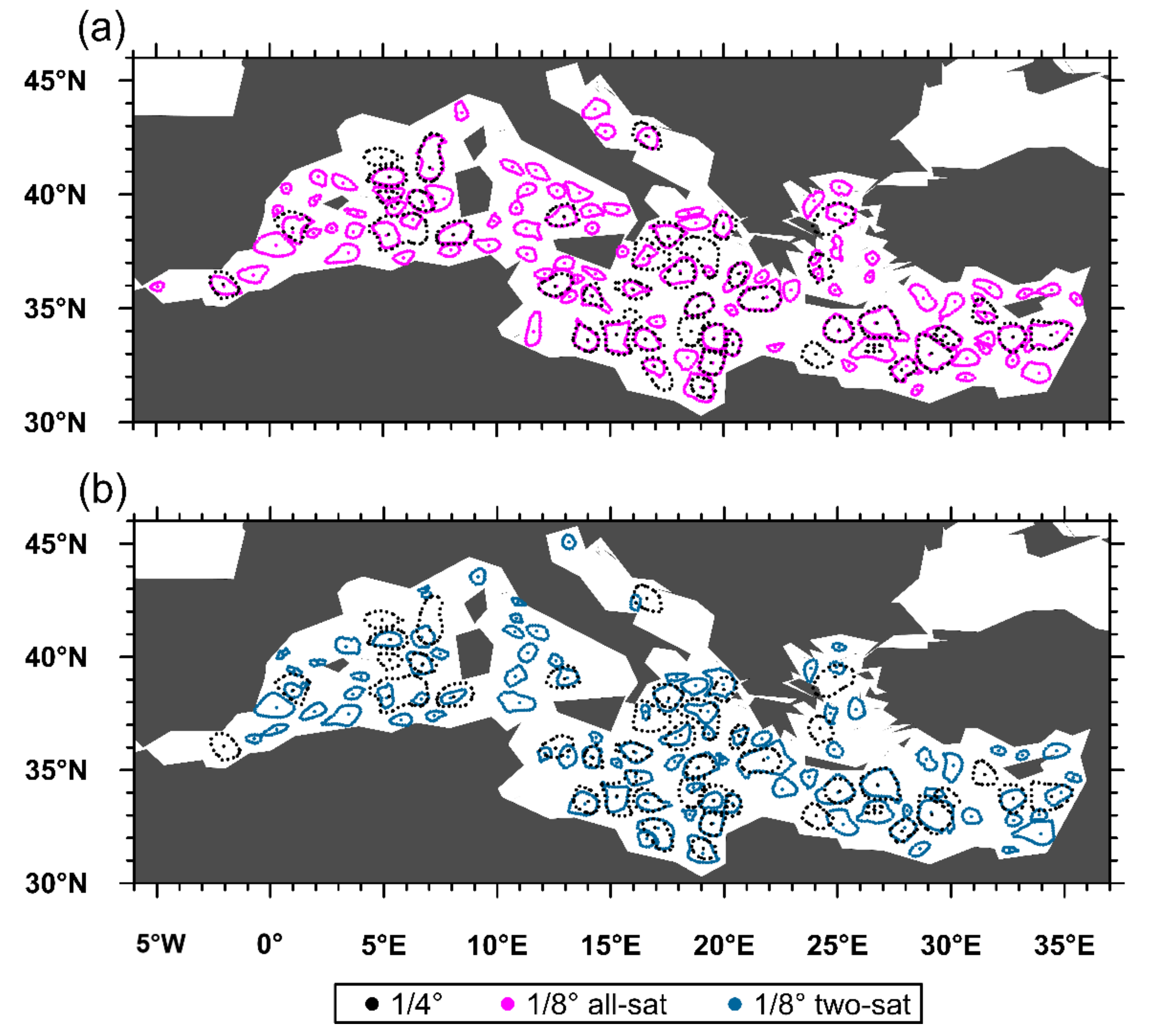
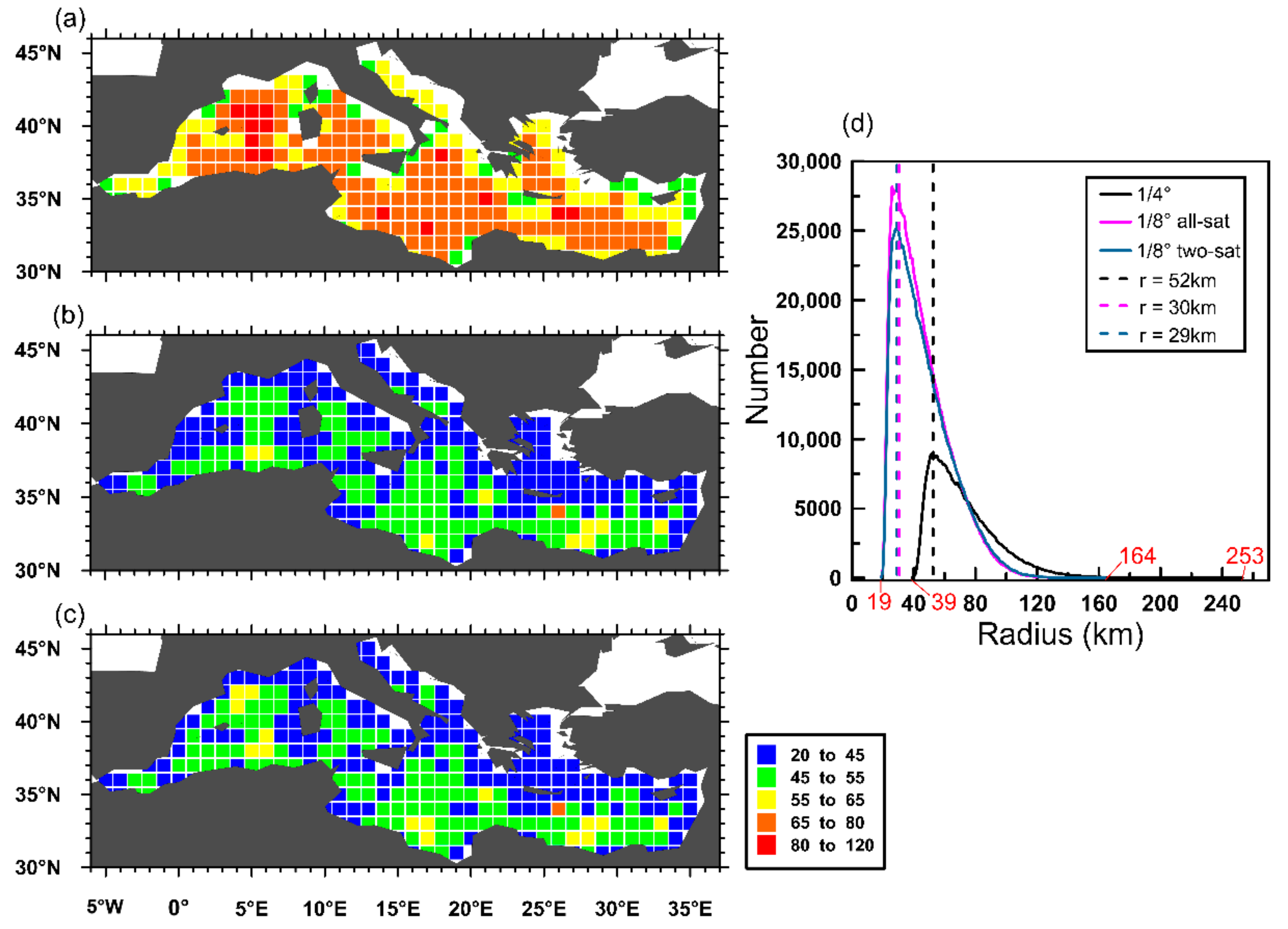
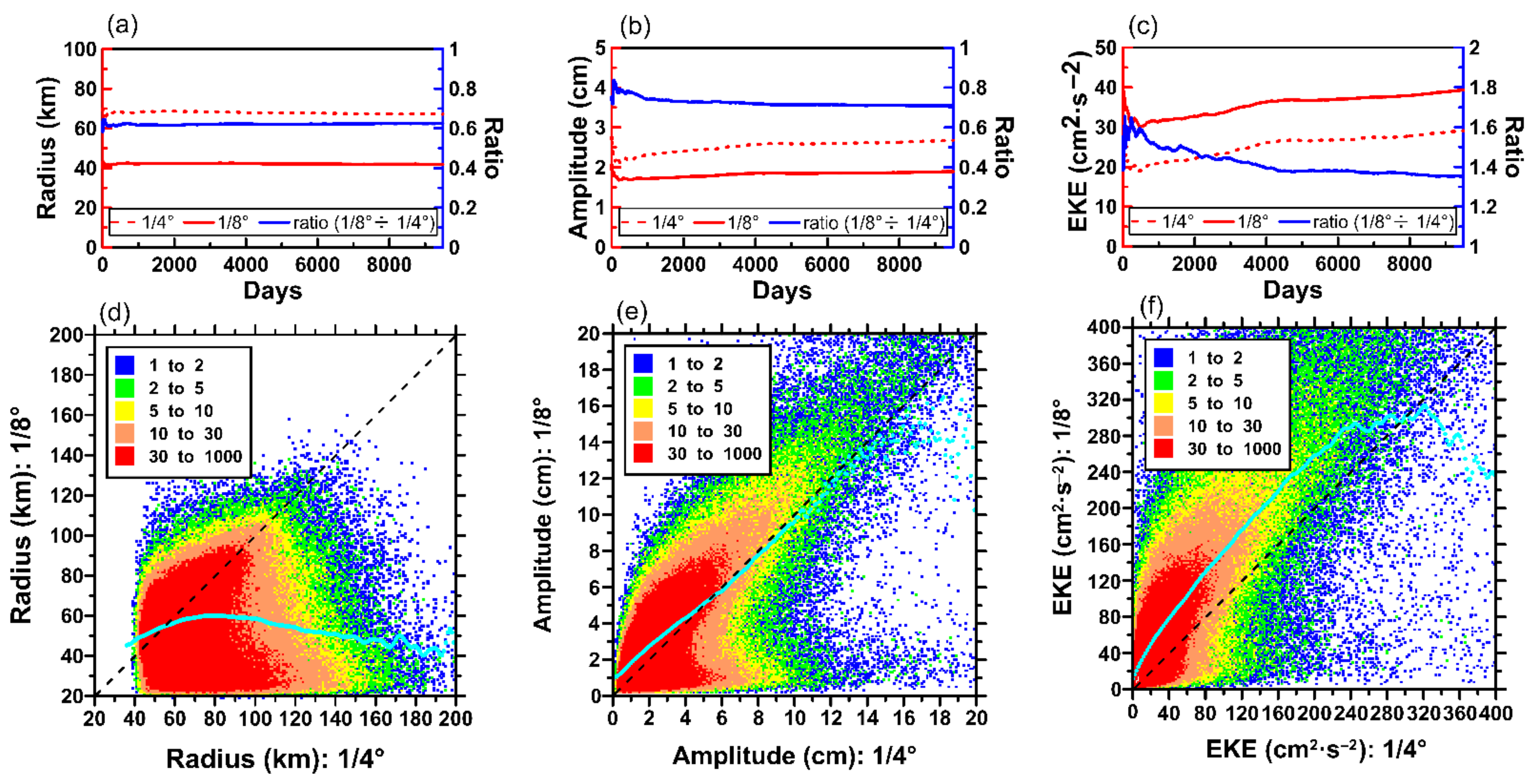
3.1. Eddy Identification in the Mediterranean Sea

The results of eddy identification using the two spatial resolutions and types of data in the Mediterranean Sea are shown in Figure 2. It can be seen that the number and density of eddies identified using the 1/8° data are larger than those identified using the 1/4°, and generally have smaller radii. The shape of eddies detected using the high-resolution data is closer to an egg-like shape: i.e., a very good approximation to a mathematical ellipsoid with a semi-major and semi-minor axis of 87.0 km and 54.0 km respectively [52]. Some parameters describing the eddy identification are presented in Table 3, including the average daily eddy number, eddy density, and the median of the eddy radii, amplitude, EKE, and eccentricity.
The eddy density is calculated based on a 1° × 1° grid. In the Mediterranean Sea, the number and density of 1/8° eddies are about 2.5 times that of 1/4° eddies, and numbers derived when using the all-sat dataset are slightly larger than when using the two-sat data. We also calculate the eddy frequency of occurrence in each 1° × 1° grid, which can be regarded as the visualization pattern of density. Figure 3 shows that the density distribution results are similar for the different spatial resolutions, but the range of values is different. The northwestern region has the lower density: <0.2 (0.4) eddy per 1° × 1° grid per day using the 1/4° (1/8°) resolution data, especially in the Adriatic, the Ionian Sea, and the Levantine Basins. The North African coasts have higher densities: >0.2 (0.4) eddy per 1° × 1° grid per day using the 1/4° (1/8°) resolution data. On the other hand, as illustrated by the pie chart, the area proportion of the eddy density in the range of 0–0.17 derived using the 1/8° resolution data is about 0.4 times that derived using the 1/4° resolution data, which shows that the areal proportion of low-density areas decreases with an increase in data resolution. The dominant density ranges of the two sets of data are 0–0.34 (1/4°) and 0.34–0.9 (1/8°), respectively.
The eddy radius presented in Table 3 is the median of the statistical series of all radii obtained over the study period. The radii for eddies identified using the 1/4° data are around 67 km, while those obtained using the 1/8° data are around 42 km (all-sat) and 43 km (two-sat) in the Mediterranean Sea. The ratio of the eddy radii identified using the 1/8° data to the 1/4° data is about 0.6. The radii derived for eddies using all-sat and two-sat products are almost the same. The average radii of all eddies in each 1° × 1° grid are also calculated. In the Mediterranean Sea, the distribution of eddy radii (Figure 4a–c) is similar to that of density to some extent. The eddies along the northern coast generally have smaller radii. On the contrary, the regions with larger radii are concentrated in the south, especially in the Algerian current and the Libyo–Egyptian current in the Mediterranean Sea. Hence, it appears that eddy radius decreases with increasing latitude, which is in line with the change in the Rossby radius of deformation [53]. The reliability of eddy detection with 1/8° data is further verified. Besides, the radii of eddies identified with 1/4° data are larger (65–120 km) than that with 1/8° data (20–55 km). As shown in the histogram of Figure 4d, the minimum (maximum) radii of eddies identified using the 1/4° data and 1/8° data are 39 km (253 km) and 19 km (164 km), respectively. The peak radii of the 1/4° eddies (~52 km) are consistently larger than the 1/8° eddy radii for both all-sat (~30 km) and two-sat (~29 km) products. The ratios of the minimum, maximum, and peak values of the two spatial resolutions data are all around 0.5–0.6, which is almost equal to the ratio of the median of their radius value. In addition, the patterns of eddy radius identified by all-sat and two-sat products are almost the same. In a sense, the improved resolution of satellite altimetry data shows a better ability to capture small-scale eddies.
The time series statistics and ratio scatter diagrams of three parameters (eddy radius, eddy amplitude, EKE) from the Mediterranean Sea are shown in Figure 5. It is worth noting that the time series statistics use the complete dataset, which includes all eddies identified using two spatial resolution data sets, while the ratio scatter diagrams used the eddy matching dataset, which contains only the eddies that can be detected using both resolutions (see Section 3.3). In addition, since the results from the all-sat and two-sat data sets are similar in these analyses, we only show those of the all-sat products. In the whole time series from the Mediterranean Sea, the daily average of radii derived from the two sets of data show a stable trend (Figure 5a), with values of about 67 km (1/4°) and 42 km (1/8°).
The ratio of the radii from the two sets of data is about 0.6, which is the same as that of the median radii (Table 3). Figure 5d shows that the radii of 1/4° eddies are still larger than those of 1/8° eddies in more cases for the matching eddy dataset. As for the amplitude, the ratios of the two resolutions are both about 0.7, similar to the ratio of the median values in Table 3. However, the eddies in the matching dataset with two resolutions have similar amplitude values. This can be explained as follows. For the median and daily mean amplitudes of all eddies, the difference between the results from the two sets of data is caused by the small eddies identified by the 1/8° data. However, the situation for EKE is the opposite as the larger the EKE, the more eddies there are in the higher resolution. For EKE, the ratio of the two resolutions is about 1.3, which is due to the calculation of EKE depending on the area of a single eddy. As for the eccentricity of the eddy, it can be seen from Table 3 that the data resolution does not affect this property and values are all close to 0.78 [52].

3.2. Eddy Tracking in the Mediterranean Sea

We tracked eddies in the Mediterranean Sea from 1993 to 2018. Previous studies have suggested that estimated lifetimes and propagation distances of regional eddies will increase with increased spatial resolution [31]. Therefore, here we focused on the longest living individual anticyclonic and cyclonic eddies, and robust eddies with long propagation distances (Figure 6). It is found that the positions of the longest-lived eddies in the Mediterranean Sea are almost the same derived from the different spatial resolution and type of datasets (anticyclonic eddy: 35°N, 22°E; cyclonic eddy: 35°N, 27°E), as shown by the red and blue stars in Figure 6. We speculate that the physical activities near this area are relatively stable, resulting in short eddy propagation distances and high stability. Obviously, this is independent of the resolution of the data.
The life spans of eddies are also shown in the insert text boxes in Figure 6. It is worth noting that although the data resolution has little effect on the position of long-lived eddies (defined by Chen et al. [54] as eddies with lifetimes longer than one year), it has a great influence on the length of eddy life. The eddies tracked by the low-resolution data may be missed for a while, and the same eddies are erroneously identified as new ones when they are observed again, which leads to the disconnection of these eddies’ life spans. Therefore, the lifetimes of eddies tracked using the low-resolution data are sometimes shorter than those obtained using the high-resolution data, especially for long-lived eddies.
The inserted figures on the left side of Figure 6 show the two large anticyclonic and cyclonic eddies with long propagation distances which occurred on 4 June 2002 and 30 January 2018, respectively. The visualization results of the three datasets are shown separately. It can be observed that the eddy tracked using the 1/4° data has a larger radius and shorter propagation distance. Moreover, the tracking accuracy using the two-sat data is better than that using the all-sat data, which is a reasonable result based on their different altimetry principles.

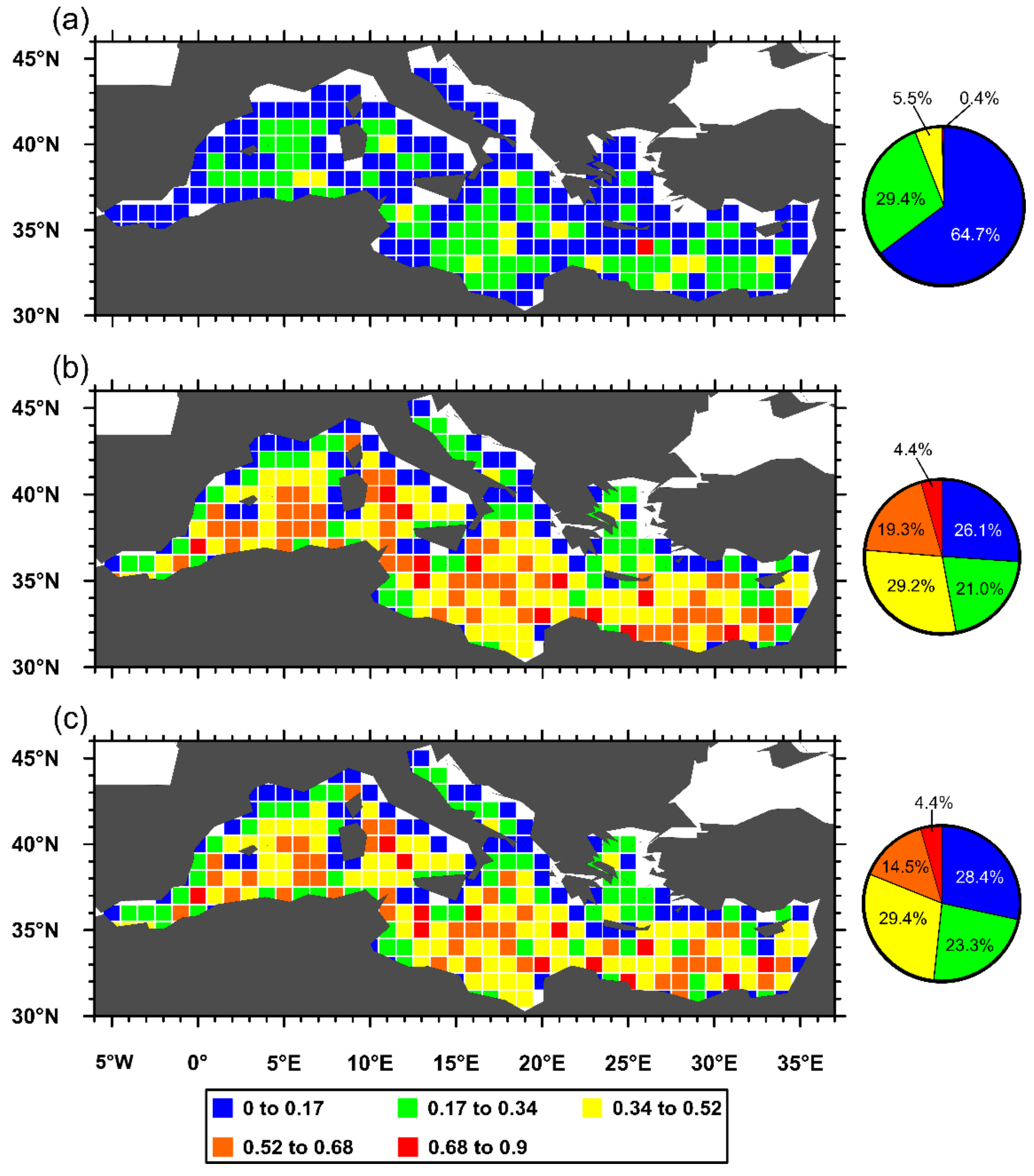
3.3. Eddy Matching in the Mediterranean Sea

Results so far have suggested that the accuracy of high-resolution data is greater than that of low-resolution in eddy identification and tracking. Eddy matching can intuitively show the advantages of resolution improvement on eddy detection. The visualization patterns of the four situations described in Section 2.2.3 are shown in Figure 7, and the probabilities of eddy matching are presented in Table 4.
It can be seen that ~70% of the 1/4° eddies can match 1/8° eddies without considering the accuracy of the parameters (Figure 7b). As shown in the density distribution maps (Figure 8a,e), most of the “correct eddies” (Situation A) are distributed in the center of the enclosed sea, and their density distribution is consistent with that of the overall eddy density.
The causes of Situation B may be the misunderstanding closure of 1/4° SLA contours caused by some specific influences (Figure 7c). We need more in-depth analysis to judge whether there is a leakage of 1/8° eddy. The probability values of Situation B (Table 4) using the two-sat data are higher than that when using the all-sat data because of their orbital observation principles. The two-sat model pays more attention to the identification and tracking of the single robust eddies, which makes it easier to miss small or complex eddies that are not easily identified. Compared with the overall distribution of eddy density, the distributions of “redundant eddies” using the all-sat in the Mediterranean Sea appear opposite, while the distribution using the two-sat data appears similar (Figure 8b,f).
Eddy identification using the 1/4° data may confuse several small eddies into a large one (Situation C), which is one of the important reasons for the lower numbers and larger radii of 1/4° eddies (Figure 7c). As can be seen in the density distribution maps (Figure 8c,g), the pattern of Situation C in the Mediterranean Sea is like that of the eddy density.
The first three situations are matched based on 1/4° eddies. Since the radii of 1/8° eddy are generally smaller than those of 1/4° eddies, there may be no eddy core of a 1/4° eddy within a 1/8° eddy, even if the two sets of data have identified the same eddy. The accurate search range for an external eddy core has not yet been determined and needs further analysis. Thus, we have only conducted one matching based on 1/8° eddies (Situation D). These 1/4° eddies should have existed but did not actually. This situation can most intuitively reflect the superiority of 1/8° data. It can be observed from the results of eddy visualization (Figure 7d), that the missing eddies have small radii and are distributed near the coastline or in complex islands (Figure 8d,h). The large interval of 1/4° SLA contours and their closed structure make it difficult for eddies to form or be detected in the presence of complex obstacles. In terms of the probability (Table 4), the values in the Mediterranean Sea are both about 0.63 using the all-sat and two-sat data products.

4. Discussion

Here we apply the methods developed for the Mediterranean Sea to three test regions: the South-China Sea; the North-West Pacific; and the South-East Pacific. The basic parameters used to describe eddies in the Mediterranean Sea (Table 3) are also presented for the three test regions (Table 5).
Compared to the values from the Mediterranean Sea, there are fewer lower ratios (1/8° ÷ 1/4°) in the number and density of eddies: i.e., around 1.5 in the South-China Sea and 1.7 in the Pacific. This may be related to their different data sources and ocean characteristics. However, the average ratio, which is close to 1.5–2.5, is likely because the precision of the 1/8° data is twice of the 1/4°.
The density distribution patterns show that the eddy density in the South-China Sea gradually decreases from northeast to southwest along a diagonal (Figure 9(Aa,Ab)). In the North-West Pacific, the East-China Sea, the Sea of Japan, and the Pacific Ocean northeast of Japan have high densities (Figure S1A). There are no obvious features in the South-East Pacific (Figure S1B). From the area proportions of the eddy density values described by the pie charts of the three areas (Figure 9(Ac); Figure S1), it can be seen that the proportion of low-density areas decreases with increasing spatial resolution.
Median eddy radii are presented in Table 5. The values derived when using the 1/4° data for the three regions (the South-China Sea; the North-West Pacific; and the South-East Pacific) are around 72 km, 77 km, and 79 km, respectively, while the values derived from the 1/8° data are around 48 km, 47 km, and 49 km, respectively. The ratios of the values derived from the two sets of data are all-around 0.6 (1/8° ÷ 1/4°), which is the same as those in the Mediterranean Sea.
We also calculate the average radii of all eddies in each 1° × 1° grid. In the South-China Sea and North-West Pacific, the patterns of eddy radii are somewhat different from that of density. The eddies with the largest radii are in the midwest of the South-China Sea (Figure 9(Ba,Bb)), which does not coincide with the highest density which is located in the northeast. In the North-West Pacific, the largest radii usually occur in the body of the Pacific Ocean to the east of Japan (Figure S2A). The eddy radius distribution in the South-East Pacific also has no significant characteristics similar to the eddy density distribution (Figure S2B).
As shown in the histograms of Figure 9(Bc) and Figure S2(Ac),(Bc), the minimum radii of eddies identified using the 1/4° and 1/8° data in the three regions are 38 km (18 km), 40 km (19 km), and 38 km (19 km), respectively. The maximum radii are 314 km (148 km), 320 km (190 km), and 239 km (165 km), respectively. The ratios of the minimum, maximum, and peak values of the two sets of data are all-around 0.5, which is the same as that for the Mediterranean Sea.
Time series statistics and ratio scatter diagrams have been calculated in the three test regions (Figure S3). Over the whole time series, the three parameters (eddy radius; eddy amplitude; EKE) in these regions present a stable trend, which suggests that there is no obvious fluctuation in the daily average value of eddy parameters. The ratios between the two resolution data are all about 0.6. Eddies in the three regions have similar radii when derived using the two sets of data: 75 km (1/4°) and 48 km (1/8°) and are a little larger than those found in the Mediterranean Sea. The ratio scatter diagrams of eddy radius (Figure S3(Ad,Bd,Cd)) also show that 1/4° eddies have larger radii than 1/8° eddies.
The median amplitude of the 1/4° eddies in the South-China Sea is similar to that of the Mediterranean Sea, being about 2.6 cm, while that of the 1/8° eddies in the latter region has larger values and the values of the other two regions are larger, and the North-West Pacific values are close to twice as large as those of the South-East Pacific. It can be inferred from this that eddy amplitude is closely related to the ocean topography. Compared with the open sea areas, the enclosed sea with complex conditions, usually have smaller parameter values. The ratio scatter diagrams for eddy radius (Figure S3(Ae,Be,Ce)) have shown that the amplitudes of 1/4° eddies are slightly larger than those of 1/8° eddies. They also show that the small-scale eddies identified using the 1/8° data pull down the mean values of the overall eddies.
As for the EKE, there are some anomalies in these three test regions: the higher the resolution, the lower the EKE. We attribute the anomalies to insufficient data and no pixel screening, and hence further exploration is needed. In addition, the South-China Sea and the North-West Pacific have larger values, while the South-East Pacific has the lowest values, which are closed in value to those of the Mediterranean Sea. This may be because this sea area which exhibits more ocean dynamics has greater EKE. Their ratio scatter diagrams (Figure S3(Af,Bf,Cf)) show that the EKE are almost the same for the two sets of data from the matching dataset. In general, the improvement of data resolution increases the accuracy of eddy parameters, and differences in these values between the two sets of data are caused by the small-scale eddies identified using the 1/8° data.
The probabilities and the patterns of the four situations (See Section 2.2.3) in the three regions are presented in Table 6 and Figure 10. Compared with the Mediterranean Sea, the values of Situation A eddies are larger, which may be due to the complex island distribution and tortuous sea-land boundary of the Mediterranean Sea. The density distribution patterns of “correct eddies” are similar to their overall eddy density. The probabilities of Situation B (Table 4 and Table 6) show that the Mediterranean Sea and the South-China Sea are relatively high at about 0.18, which are around three times those of the Pacific which are about 0.06. Compared with the overall eddy density, the distributions of “redundant eddies” (Situation B) from the all-sat data in the Mediterranean Sea and the South-China are opposite (Figure 8b and Figure 11(Ab)), while the two-sat and the North-West Pacific distributions are similar (Figure 8f and Figure 11(Bb)). The regularity of the South-East Pacific is not so obvious (Figure 11(Cb)).
As for Situation C, the Mediterranean Sea has the highest values as can be seen from Table 4 and Table 6. There may be two reasons for this: one is that the Mediterranean data source is different from the other three test regions, which may affect the processing accuracy; the other is because of the complex island distribution and winding coastline in the Mediterranean Sea. As shown in the density distribution maps (Figure 11), the patterns in the Mediterranean Sea, the South-China Sea, and the North-West Pacific are like those of their eddy density, although in the South-East Pacific eddy density is higher in the west and lower in the east. Values for Situation D eddies in the Mediterranean Sea are higher than those of the three test regions. We believe that the reasons for this are consistent with the explanations for Situations A, B, and C.

5. Conclusions

In this paper, we analyze the impact of the resolution improvement of satellite altimetry data on eddy research. Four sea areas: the Mediterranean Sea, the South-China Sea, the North-West Pacific, and the South-East Pacific are selected for the study. Using the same eddy identification and tracking algorithms, we analyze the characteristics of eddies under two spatial resolutions (1/4° and 1/8°) and data types (all-sat and two-sat in the Mediterranean Sea) data sets, yielding the following main results,
Firstly, our results show that the number and density of eddies identified using the 1/8° data are twice as great as those identified using the 1/4° data. This is consistent with the generation principle of 1/8° data. The 1/8° data used in this paper is obtained by spatial interpolation on the basis of 1/4° data. The observation grid is reduced from 0.25° × 0.25° to 0.125° × 0.125°, and the accuracy is doubled in the unilateral direction to obtain more precise results. The eddies identified by 1/8° data generally have smaller radii, amplitudes, and larger EKE values, and the ratios of these parameters between the two spatial resolutions are around 0.6–0.8 and 1.3 (1/8° ÷ 1/4°).
With the improvement in spatial resolution, not only may the eddy parameters be closer to the true values but more small-scale eddies can be captured, which plays an important role in the accurate approximation of eddy parameter values. The differences in parameters between the two resolutions are mainly caused by the small-scale eddies identified using the 1/8° data, especially for the amplitude and EKE parameters. This is of great significance for the future study of ocean dynamics and ecology.
Secondly, the tracking results show that the improvement of data resolution has little effect on the distribution position of anticyclonic or cyclonic long-lived eddies, but has a great effect on the length of their life. Similarly, the values of propagation distances of eddies are also affected by the data resolution. The higher the resolution, the longer the eddy life and the propagation distance, which is the inevitable result of the improvement in the continuous eddy capturing capability.
Thirdly, the eddy matching results show that without considering the difference of characteristics, ~70% to 80% of the 1/4° eddies are correct, and ~20% to 30% are redundant or confused. The 1/4° identified eddies only account for ~30% to 60% of the eddies identified using the high-resolution data, which suggests that the 1/4° resolution will result in most of the small-scale eddies being missed.
Fourthly, our study shows that the all-sat data have stronger eddy capture ability and more accurate eddy characteristic analysis potential for most eddies. While the two-sat data have better eddy capture and eddy tracking ability for a single robust eddy.
Finally, the differences in eddy characteristics in four sea areas (the Mediterranean Sea and three test regions) are systematically evaluated. For an enclosed sea with complex conditions such as the Mediterranean Sea and the South-China Sea, the data resolution has a greater impact on it. Low-resolution data tends to miss more existing eddies, thus affecting the research results. However, the distribution trend of this kind of sea area is more obvious and it has stronger regional characteristics. On the contrary, the regional characteristics of the relatively open Pacific Ocean are not very obvious, and the improvement of data accuracy has less impact on the eddy studies there.

Supplementary Materials

The following supporting information can be downloaded at: https://www.mdpi.com/article/10.3390/rs14010149/s1, Figure S1: Eddy density distribution maps and density ratio pie charts in the North-West Pacific and the South-East Pacific; Figure S2: Eddy radius distribution maps and radius line charts in the North-West Pacific and the South-East Pacific; Figure S3: Time series statistics and ratio scatter diagrams of three parameters (eddy radius, eddy amplitude, and EKE) in the South-China Sea, the North-West Pacific, and the South-West Pacific.

Author Contributions

Conceptualization, Y.W. and J.Y.; methodology, Y.W. and X.C.; software, Y.W.; validation, Y.W.; formal analysis, Y.W.; investigation, Y.W., X.C., G.H., P.J. and J.Y.; writing—original draft preparation, Y.W.; writing—review and editing, Y.W., X.C., G.H., P.J. and J.Y.; visualization, Y.W.; supervision, X.C., G.H., P.J. and J.Y.; project administration, J.Y.; funding acquisition, J.Y. All authors have read and agreed to the published version of the manuscript.”

Funding

This research was jointly supported by the Natural Science Foundation of China (Grant No. 42030406), the Ministry of Science and Technology of China (Grant No. 2019YFD0901001), and the ESA-NRSCC Scientific Cooperation Project on Earth Observation Science and Applications: Dragon 5 (Grant No. 58393).

Institutional Review Board Statement

Not applicable.

Informed Consent Statement

Not applicable.

Data Availability Statement

The data used in this study is available as follows. The sea level anomaly (SLA) data with 1/4° and 1/8° resolution in the Mediterranean Sea used in this study is delayed-time products distributed by CMEMS (Copernicus Marine and Environment Monitoring Service, marine.copernicus.eu). The high precision fusion data of the other three regions (the South-China Sea, the North-West Pacific and the South-East Pacific) was purchased from the Data Unification and Altimeter Combination System (DUACS). The whole eddy dataset identified using the 1/4° data can be obtained from http://coadc.ouc.edu.cn/tfl/ and http://data.casearth.cn/ (Data ID: XDA19090202; Accessed date: 15 September 2021).

Conflicts of Interest

The authors declare no conflict of interest.

References

  1. Chelton, D.B.; Schlax, M.G.; Samelson, R.M. Global Observations of Nonlinear Mesoscale Eddies. Prog. Oceanogr. 2011, 91, 167–216. [Google Scholar] [CrossRef]
  2. Fu, L.L. Pattern and Velocity of Propagation of the Global Ocean Eddy Variability. J. Geophys. Res.-Ocean. 2009, 114, C11017. [Google Scholar] [CrossRef] [Green Version]
  3. Cheng, Y.H.; Ho, C.R.; Zheng, Q.; Kuo, N.J. Statistical Characteristics of Mesoscale Eddies in the North Pacific Derived from Satellite Altimetry. Remote Sens. 2014, 6, 5164–5183. [Google Scholar] [CrossRef] [Green Version]
  4. Raffaele, F.; Wunsch, C. The Distribution of Eddy Kinetic and Potential Energies in the Global Ocean. Tellus A 2010, 62, 92–108. [Google Scholar] [CrossRef]
  5. Bennett, A.F.; White, W.B. Eddy Heat Flux in the Subtropical North Pacific. J. Phys. Oceanogr. 1986, 16, 728–740. [Google Scholar] [CrossRef]
  6. Roemmich, D.; Gilson, J. Eddy Transport of Heat and Thermocline Waters in the North Pacific: A Key to Interannual/Decadal Climate Variability. J. Phys. Oceanogr. 2001, 31, 675–687. [Google Scholar] [CrossRef]
  7. Johnson, K.S.; Riser, S.C.; Karl, D.M. Nitrate Supply from Deep to Near-Surface Waters of the North Pacific Subtropical Gyre. Nature 2010, 465, 1062–1065. [Google Scholar] [CrossRef] [PubMed]
  8. Dong, C.; McWilliams, J.C.; Liu, Y.; Chen, D. Global Heat and Salt Transports by Eddy Movement. Nat. Commun. 2014, 5, 3294. [Google Scholar] [CrossRef] [Green Version]
  9. Thompson, A.F.; Heywood, K.J.; Schmidtko, S.; Stewart, A.L. Eddy Transport as a Key Component of the Antarctic Overturning Circulation. Nat. Geosci. 2014, 7, 879–884. [Google Scholar] [CrossRef]
  10. McGillicuddy, D.J.; Dennis, J. Mechanisms of Physical-Biological-Biogeochemical Interaction at the Oceanic Mesoscale. Annu. Rev. Mar. Sci. 2016, 8, 125–159. [Google Scholar] [CrossRef] [PubMed] [Green Version]
  11. Melnichenko, O.; Amores, A.; Maximenko, N.; Hacker, P.; Potemra, J. Signature of Mesoscale Eddies in Satellite Sea Surface Salinity Data. J. Geophys. Res.-Ocean. 2017, 122, 1416–1424. [Google Scholar] [CrossRef]
  12. Chelton, D.B.; Gaube, P.; Schlax, M.G.; Early, J.J.; Samelson, R.M. The Influence of Nonlinear Mesoscale Eddies on Near-Surface Oceanic Chlorophyll. Science 2011, 334, 328–332. [Google Scholar] [CrossRef]
  13. Gaube, P.; Chelton, D.B.; Samelson, R.M.; Schlax, M.G.; O’Neill, L.W. Satellite Observations of Mesoscale Eddy-Induced Ekman Pumping. J. Phys. Oceanogr. 2015, 45, 104–132. [Google Scholar] [CrossRef]
  14. Villas Bôas, A.B.; Sato, O.T.; Chaigneau, A.; Castelão, G.P. The Signature of Mesoscale Eddies on the Air-Sea Turbulent Heat Fluxes in the South Atlantic Ocean. Geophys. Res. Lett. 2015, 42, 1856–1862. [Google Scholar] [CrossRef]
  15. Ma, X.; Chang, P.; Liu, X.; Montuoro, R.; Small, R.J.; Bryan, F.O.; Greatbatch, R.J.; Brandt, P.; Wu, D. Western Boundary Currents Regulated by Interaction between Ocean Eddies and the Atmosphere. Nature 2016, 535, 533–537. [Google Scholar] [CrossRef] [PubMed]
  16. Fu, L.L.; Chelton, D.B.; Traon, P.Y.L.; Morrow, R. Eddy Dynamics from Satellite Altimetry. Oceanography 2010, 23, 14–25. [Google Scholar] [CrossRef] [Green Version]
  17. Stumpf, H.G.; Legeckis, R.V. Satellite Observations of Mesoscale Eddy Dynamics in the Eastern Tropical Pacific Ocean. J. Phys. Oceanogr. 1977, 7, 648–658. [Google Scholar] [CrossRef] [Green Version]
  18. Chelton, D.B.; Schlax, M.G.; Samelson, R.M.; de Szoeke, R.A. Global Observations of Large Oceanic Eddies. Geophys. Res. Lett. 2007, 34, L15606. [Google Scholar] [CrossRef]
  19. D’Alimonte, D. Detection of Mesoscale Eddy-Related Structures through Iso-SST Patterns. IEEE Geosci. Remote Sens. Lett. 2009, 6, 189–193. [Google Scholar] [CrossRef]
  20. Dong, C.; Nencioli, F.; Liu, Y.; McWilliams, J.C. An Automated Approach to Detect Oceanic Eddies from Satellite Remotely Sensed Sea Surface Temperature Data. IEEE Geosci. Remote Sens. Lett. 2011, 8, 1055–1059. [Google Scholar] [CrossRef]
  21. Gonzalez-Silvera, A.; Santamaria-del-Angel, E.; Millán-Nuñez, R.; Manzo-Monroy, H. Satellite Observations of Mesoscale Eddies in the Gulfs of Tehuantepec and Papagayo (Eastern Tropical Pacific). Deep-Sea Res. Part II 2004, 51, 587–600. [Google Scholar] [CrossRef]
  22. Park, J.E.; Park, K.A.; Ullman, D.S.; Cornillon, P.C.; Park, Y.J. Observation of Diurnal Variations in Mesoscale Eddy Sea-Surface Currents Using GOCI Data. Remote Sens. Lett. 2016, 7, 1131–1140. [Google Scholar] [CrossRef] [Green Version]
  23. Du, Y.; Song, W.; He, Q.; Huang, D.; Liotta, A.; Su, C. Deep Learning with Multi-Scale Feature Fusion in Remote Sensing for Automatic Oceanic Eddy Detection. Inf. Fusion 2019, 49, 89–99. [Google Scholar] [CrossRef] [Green Version]
  24. Carsey, F.D.; Garwood, R.W. Identification of Modeled Ocean Plumes in Greenland Gyre ERS-1 SAR Data. Geophys. Res. Lett. 1993, 20, 2207–2210. [Google Scholar] [CrossRef]
  25. Rouault, M.J.; Mouche, A.; Collard, F.; Johannessen, J.A.; Chapron, B. Mapping the Agulhas Current from Space: An Assessment of ASAR Surface Current Velocities. J. Geophys. Res.-Ocean. 2010, 115, C10026. [Google Scholar] [CrossRef] [Green Version]
  26. Chen, G.; Chen, X.; Huang, B. Independent Eddy Identification with Profiling Argo as Calibrated by Altimetry. J. Geophys. Res.-Ocean. 2021, 126, e2020JC016729. [Google Scholar] [CrossRef]
  27. Robinson, A.R. Overview and Summary of Eddy Science. In Eddies in Marine Science; Robinson, A.R., Ed.; Springer: Berlin/Heidelberg, Germany, 1983; Volume 609, pp. 3–15. [Google Scholar] [CrossRef]
  28. Faghmous, J.H.; Frenger, I.; Yao, Y.; Warmka, R.; Lindell, A.; Kumar, V. A Daily Global Mesoscale Ocean Eddy Dataset from Satellite Altimetry. Sci. Data 2015, 2, 150028. [Google Scholar] [CrossRef] [Green Version]
  29. Frenger, I.; Gruber, N.; Knutti, R.; Münnich, M. Imprint of Southern Ocean Eddies on Winds, Clouds and Rainfall. Nat. Geosci. 2013, 6, 608–612. [Google Scholar] [CrossRef]
  30. Zhang, Z.; Wang, W.; Qiu, B. Oceanic Mass Transport by Mesoscale Eddies. Science 2014, 345, 322–324. [Google Scholar] [CrossRef]
  31. Amores, A.; Jordà, G.; Arsouze, T.; Le Sommer, J. Up to What Extent Can We Characterize Ocean Eddies Using Present-Day Gridded Altimetric Products? J. Geophys. Res.-Ocean. 2018, 123, 7220–7236. [Google Scholar] [CrossRef]
  32. Xu, Y.; Fu, L.L. The Effects of Altimeter Instrument Noise on the Estimation of the Wavenumber Spectrum of Sea Surface Height. J. Phys. Oceanogr. 2012, 42, 2229–2233. [Google Scholar] [CrossRef] [Green Version]
  33. Dufau, C.; Orsztynowicz, M.; Dibarboure, G.; Morrow, R.; Le Traon, P.-Y. Mesoscale Resolution Capability of Altimetry: Present and Future. J. Geophys. Res.-Ocean. 2016, 121, 4910–4927. [Google Scholar] [CrossRef] [Green Version]
  34. Treguier, A.M.; Deshayes, J.; Lique, C.; Dussin, R.; Molines, J.M. Eddy Contributions to The Meridional Transport of Salt in the North Atlantic. J. Geophys. Res.-Ocean. 2012, 177, C05010. [Google Scholar] [CrossRef] [Green Version]
  35. Mkhinini, N.; Coimbra, A.L.S.; Stegner, A.; Arsouze, T.; Taupier-Letage, I.; Béranger, K. Long-Lived Mesoscale Eddies in the Eastern Mediterranean Sea: Analysis of 20 Years of AVISO Geostrophic Velocities. J. Geophys. Res.-Ocean. 2014, 119, 8603–8626. [Google Scholar] [CrossRef]
  36. Escudier, R.; Renault, L.; Ananda, P.; Pierre, B.; Chelton, D.; Jonathan, B. Eddy Properties in the Western Mediterranean Sea from Satellite Altimetry and a Numerical Simulation. J. Geophys. Res.-Ocean. 2016, 121, 3990–4006. [Google Scholar] [CrossRef]
  37. Le, V.B.; Stegner, A.; Arsouze, T. Angular Momentum Eddy Detection and Tracking Algorithm (AMEDA) and Its Application to Coastal Eddy Formation. J. Atmos. Ocean. Technol. 2018, 35, 739–762. [Google Scholar] [CrossRef]
  38. Morrow, R.; Fu, L.L.; Ardhuin, F.; Benkiran, M.; Chapron, B.; Cosme, E.; D’Ovidio, F.; Farrar, J.T.; Gille, S.T.; Lapeyre, G.; et al. Global Observations of Fine-Scale Ocean Surface Topography With the Surface Water and Ocean Topography (SWOT) Mission. Front. Mar. Sci. 2019, 6, 232. [Google Scholar] [CrossRef]
  39. Pujol, M.I.; Faugère, Y.; Taburet, G.; Dupuy, S.; Pelloquin, C.; Ablain, M.; Picot, N. DUACS DT2014: The New Multi-Mission Altimeter Data Set Reprocessed over 20 Years. Ocean. Sci. 2016, 12, 1067–1090. [Google Scholar] [CrossRef] [Green Version]
  40. Doglioli, A.M.; Blanke, B.; Speich, S.; Lapeyre, G. Tracking Coherent Structures in a Regional Ocean Model with Wavelet Analysis: Application to Cape Basin Eddies. J. Geophys. Res.-Ocean. 2007, 112, C05043. [Google Scholar] [CrossRef] [Green Version]
  41. Chaigneau, A.; Gizolme, A.; Grados, C. Mesoscale Eddies off Peru in Altimeter Records: Identification Algorithms and Eddy Spatio-Temporal Patterns. Prog. Oceanogr. 2008, 79, 106–119. [Google Scholar] [CrossRef]
  42. Williams, S.; Hecht, M.; Petersen, M.; Strelitz, R.; Maltrud, M.; Ahrens, J.P.; Hlawitschka, M.; Hamann, B. Visualization and Analysis of Eddies in a Global Ocean Simulation. Comput. Graph. Forum 2011, 30, 991–1000. [Google Scholar] [CrossRef]
  43. Haller, G.; Hadjighasem, A.; Farazmand, M.; Huhn, F. Defining Coherent Vortices Objectively from the Vorticity. J. Fluid. Mech. 2015, 795, 136–173. [Google Scholar] [CrossRef] [Green Version]
  44. Isern-Fontanet, J.; Garcia-Ladona, E.; Font, J. Identification of Marine Eddies from Altimetric Maps. J. Atmos. Ocean. Tech. 2003, 20, 772–778. [Google Scholar] [CrossRef]
  45. Penven, P.; Echevin, V.; Pasapera, J.; Colas, F.; Tam, J. Average Circulation, Seasonal Cycle, and Mesoscale Dynamics of the Peru Current System: A Modeling Approach. J. Geophys. Res.-Ocean. 2005, 110, C10021. [Google Scholar] [CrossRef]
  46. Henson, S.A.; Thomas, A.C. A Census of Oceanic Anticyclonic Eddies in the Gulf of Alaska. Deep.-Sea Res. Part I 2008, 55, 163–176. [Google Scholar] [CrossRef]
  47. Liu, Y.; Chen, G.; Sun, M.; Liu, S.; Tian, F. A Parallel SLA-Based Algorithm for Global Mesoscale Eddy Identification. J. Atmos. Ocean. Tech. 2016, 33, 2743–2754. [Google Scholar] [CrossRef]
  48. Tian, F.; Wu, D.; Yuan, L.; Chen, G. Impacts of the Efficiencies of Identification and Tracking Algorithms on the Statistical Properties of Global Mesoscale Eddies Using Merged Altimeter Data. Int. J. Remote Sens. 2020, 41, 2835–2860. [Google Scholar] [CrossRef]
  49. Arbic, B.K.; Scott, R.B.; Chelton, D.B.; Richman, J.G.; Shriver, J.F. Effects of Stencil Width on Surface Ocean Geostrophic Velocity and Vorticity Estimation from Gridded Satellite Altimeter Data. J. Geophys. Res.-Atmos. 2012, 117, 3029. [Google Scholar] [CrossRef] [Green Version]
  50. Durand, M.; Fu, L.L.; Lettenmaier, D.P.; Alsdorf, D.E.; Rodriguez, E.; Esteban-Fernandez, D. The Surface Water and Ocean Topography Mission: Observing Terrestrial Surface Water and Oceanic Submesoscale Eddies. Proc. IEEE 2010, 98, 766–779. [Google Scholar] [CrossRef]
  51. Pujol, M.I.; Dibarboure, G.; Le Traon, P.Y.; Klein, P. Using High-Resolution Altimetry to Observe Mesoscale Signals. J. Atmos. Ocean. Tech. 2013, 29, 1409–1416. [Google Scholar] [CrossRef]
  52. Chen, G.; Han, G.; Yang, X. On the Intrinsic Shape of Oceanic Eddies Derived from Satellite Altimetry. Remote Sens. Environ. 2019, 228, 75–89. [Google Scholar] [CrossRef]
  53. Chelton, D.B.; Deszoeke, R.A.; Schlax, M.G.; Naggar, K.E.; Siwertz, N. Geographical Variability of the First Baroclinic Rossby Radius of Deformation. J. Phys. Oceanogr. 1998, 28, 433–460. [Google Scholar] [CrossRef]
  54. Chen, G.; Han, G. Contrasting Short-Lived with Long-Lived Mesoscale Eddies in the Global Ocean. J. Geophys. Res.-Ocean. 2019, 124, 3149–3167. [Google Scholar] [CrossRef]
Figure 1. SLA (cm) and eddy identification results (eddy effect contour and eddy centroid core) of three datasets in the Mediterranean Sea: (a) 1/4°; (b) 1/8° all-sat; (c) 1/8° two-sat.
Remotesensing 14 00149 g001
Figure 2. Overlay maps of eddy identification with two spatial resolutions and data types in the Mediterranean Sea: (a) 1/4° and 1/8° all-sat; (b) 1/4° and 1/8° two-sat. The black dots represent eddy effect contours identified using the 1/4° data, and the magenta (desert blue) dots represent eddy effect contours identified using the 1/8° all-sat (two-sat) data.
Remotesensing 14 00149 g002
Figure 3. Eddy density distribution maps and density ratio pie charts for the Mediterranean Sea: (a) 1/4°; (b) 1/8° all-sat; (c) 1/8° two-sat. The colored squares represent the range of eddy density, as shown in the legend. The color pie charts represent the proportion of each density range.
Remotesensing 14 00149 g003
Figure 4. Eddy radius distribution maps and radius histogram of the Mediterranean Sea: (a) 1/4°; (b) 1/8° all-sat; (c) 1/8° two-sat. The colored squares represent the range of eddy radii, as shown in the legend. The histogram (d) represents the relationship between eddy radii and number in the different datasets, where the black line represents the eddies identified using the 1/4° data, and the magenta (desert blue) line represents eddies identified using the 1/8° all-sat (two-sat) data.
Remotesensing 14 00149 g004
Figure 5. Time series statistics (ac) and ratio scatter diagram (df) of three parameters in the Mediterranean Sea: (a,d) eddy radius; (b,e) eddy amplitude; (c,f) EKE. In (ac), the red dotted (solid) lines represent the daily average values of 1/4° (1/8° all-sat) eddies, corresponding to the red axis in the left, and the solid blue lines represent the ratio of the values of two resolutions, corresponding to the blue axis in the right. In (df), the abscissa (ordinate) represents the values of 1/4° (1/8°) eddies’ parameter, and the color squares represent the number of eddies that meet the point value, and their ranges are shown in the legend. The cyan lines are the two-dimension fitting of scattered points, and the black dotted lines are diagonal.
Remotesensing 14 00149 g005
Figure 6. Results from tracking typical eddies in the Mediterranean Sea. (a) represents typical anticyclonic eddies and (b) represents typical cyclonic ones. The red (blue) stars in the figure represent the location of the anticyclonic (cyclonic) eddy with the longest life in the Mediterranean Sea from 1993 to 2018. The three lifetimes indicated in the insert boxes are the tracking results based on 1/4°, 1/8° all-sat, and 1/8° two-sat datasets respectively. The shapes and trajectories of the long-distance eddies are shown in inserts on the left. The black lines represent the eddy identified using the 1/4° data, and the magenta (desert blue) lines represent the eddy identified using the 1/8° all-sat (two-sat) data.
Remotesensing 14 00149 g006
Figure 7. Visualization of eddies for four matching situations from two different resolution data sets in the Mediterranean Sea. The black lines represent eddy effect contours identified using the 1/4° data, and the magenta lines represent eddy effect contours identified using the 1/8° data. (a) represents all eddies identified under 1/4° and 1/8°all-sat data, (b) represents Situation A, (c) represents Situation B and C, and (d) represents Situation D. (See Section 2.2.3 for a description of the four situations).
Remotesensing 14 00149 g007
Figure 8. Density distribution of four matching situations in the Mediterranean Sea: (a,e) Situation A; (b,f) Situation B; (c,g) Situation C; (d,h) Situation D (See Section 2.2.3 for a description of the four situations). On the left are the results using the all-sat data, and on the right are the results using the two-sat data. The legend on the right shows the range of density values.
Remotesensing 14 00149 g008
Figure 9. (A) Eddy density distribution maps ((a) 1/4°; (b) 1/8°) and density ratio pie charts (c) in the South-China Sea. The colored squares represent the range of eddy density, as shown in the legend. The color pie charts represent the proportion of each density range and the result of 1/4° data is on the left. (B) Eddy radius distribution maps ((a) 1/4°; (b) 1/8°) and radius line chart (c) in the South-China Sea. The colored squares represent the range of eddy radius, as shown in the legend. The histogram represents the relationship between eddy radius and number under different resolutions, where the black line represents the eddies identified using the 1/4° data, and the magenta line represents the eddies identified using the 1/8° data.
Remotesensing 14 00149 g009
Figure 10. Visualization of eddies for four matching situations of two resolution eddies in the three regions: (A) the South-China Sea; (B) the North-West Pacific; (C) the South-West Pacific. The black lines represent eddy effect contours identified by 1/4° data, and the magenta lines represent eddy effect contours identified using the 1/8° data. (a) represents all eddies identified using the 1/4° and 1/8°all-sat products, (b) represents Situation A, (c) represents Situation B and C, and (d) represents Situation D.
Remotesensing 14 00149 g010
Figure 11. Density distribution of four matching situations in the three regions: (A) the South-China Sea; (B) the North-West Pacific; (C) the South-East Pacific and (a) Situation A; (b) Situation B; (c) Situation C; (d) Situation D. The legends show the range of density values.
Remotesensing 14 00149 g011
Table 1. Details of the SLA data sets used in this study.
ResolutionCoverageRangeTime SeriesSatellitesType
1/4° × 1/4°
Daily
Global Ocean90°S–90°N
180°W–180°E
19930101–20181231All-Sat➀Gridded
1/8° × 1/8°
Daily
Mediterranean Sea30°N–46°N
6°W–37°E
All-Sat➁
Two-Sat➂
South-China Sea0°–25°N
105°E–125°E
20180101–20181231All-Sat
North-West Pacific25°N–45°N
120°E–160°E
South-East Pacific55°S–35°S
130°W–90°W
Note. CMEMS ID of the downloaded datasets: ➀ SEALEVEL_GLO_PHY_L4_REP_OBSERVATIONS_008_047. ➁ SEALEVEL_MED_PHY_L4_REP_OBSERVATIONS_008_051. ➂ SEALEVEL_MED_PHY_CLIMATE_L4_REP_OBSERVATIONS_008_056.
Table 2. Resulting from four different situations of eddy matching.
SituationABCD
1/4° eddy number1110
1/8° eddy number10>11
Table 3. Parameters describing the identified eddies in the Mediterranean Sea.
Sea AreaMediterranean Sea
resolution1/4°1/8° all-sat1/8° two-sat
Eddy number3910296
Eddy density (num·deg−2·day−1)0.150.380.35
Eddy radius (km)674243
Eddy amplitude (cm)2.681.901.86
EKE (cm2·s−2)293936
Eddy eccentricity0.770.780.78
Table 4. Probabilities of eddy matching in the Mediterranean Sea.
SituationsDatasets FoundationsMediterranean Sea
All-SatTwo-Sat
A1/4°0.720.70
B0.170.20
C0.110.10
D1/8°0.630.63
Table 5. Parameters of eddies in the three regions.
Sea AreaSouth-China SeaNorth-West PacificSouth-East Pacific
Resolution1/4°1/8°1/4°1/8°1/4°1/8°
Eddy number355494165148254
Eddy density (num·deg−2·day−1)0.090.140.140.240.190.32
Eddy radius (km)724877477949
Eddy amplitude (cm)2.551.436.183.023.431.88
EKE (cm2·s−2)162111146943123
Eddy eccentricity0.790.780.790.780.780.77
Table 6. Probabilities of eddy matching in the three regions.
SituationsDatasets FoundationsSouth-China SeaNorth-West PacificSouth-East Pacific
A1/4°0.840.880.89
B0.130.060.06
C0.030.060.05
D1/8°0.430.440.42
Publisher’s Note: MDPI stays neutral with regard to jurisdictional claims in published maps and institutional affiliations.

