Mapping Aquaculture Ponds for the Coastal Zone of Asia with Sentinel-1 and Sentinel-2 Time Series

Abstract

Asia dominates the world’s aquaculture sector, generating almost 90 percent of its total annual global production. Fish, shrimp, and mollusks are mainly farmed in land-based pond aquaculture systems and serve as a primary protein source for millions of people. The total production and area occupied for pond aquaculture has expanded rapidly in coastal regions in Asia since the early 1990s. The growth of aquaculture was mainly boosted by an increasing demand for fish and seafood from a growing world population. The aquaculture sector generates income and employment, contributes to food security, and has become a billion-dollar industry with high socio-economic value, but has also led to severe environmental degradation. In this regard, geospatial information on aquaculture can support the management of this growing food sector for the sustainable development of coastal ecosystems, resources, and human health. With free and open access to the rapidly growing volume of data from the Copernicus Sentinel missions as well as machine learning algorithms and cloud computing services, we extracted coastal aquaculture at a continental scale. We present a multi-sensor approach that utilizes Earth observation time series data for the mapping of pond aquaculture within the entire Asian coastal zone, defined as the onshore area up to 200 km from the coastline. In this research, we developed an object-based framework to detect and extract aquaculture at a single-pond level based on temporal features derived from high-spatial-resolution SAR and optical satellite data acquired from the Sentinel-1 and Sentinel-2 satellites. In a second step, we performed spatial and statistical data analyses of the Earth-observation-derived aquaculture dataset to investigate spatial distribution and identify production hotspots at various administrative units at regional, national, and sub-national scale.

1. Introduction

1.1. Asia’s Role in Global Aquaculture Production

The global increase in demand for protein-rich fish, seafood, and other fish products has led to severe overfishing of the world’s oceans and stagnating catches from marine fisheries in recent years. At the same time, aquaculture has recorded a rapid increase in production and become the fastest growing sector in the global food industry, with an average annual growth rate of 6.9 percent over the past three decades [1]. Aquaculture production has increased more than six-fold since 1990: more than 85 million tons are valued at 275 billion US dollars worldwide (according to the latest FAO statistics for the year 2019), and the aquaculture sector is becoming increasingly important as a source of income and nutrition [2,3]. Half of all edible fish are produced in offshore and onshore aquaculture systems, and demand continues to rise. Aquaculture is a major protein supplier and plays an important role in food security and the achievement of the United Nations (UN) Sustainable Development Goals (SDGs) for a growing world population of up to 10 billion people for the year 2050—as projected by the UN [4,5,6,7].

With a share of 88 percent (75 million tons) of the global total volume [1], Asia is the world’s largest regional aquaculture producer and has been the major driver of global aquaculture growth in recent years (see Figure 1). Land-based pond culture of fish and shrimp in fresh water and brackish water has a long tradition in Asia and has contributed most to Asia’s dominant role in aquaculture production. In Asia, aquaculture has expanded rapidly since the 1990s along the coasts, especially those of Southeast Asia and East Asia [8], and become a major protein source for millions of people. Aquaculture has become a billion-dollar industry with high socio-economic value, generates income and employment, and contributes to food security. However, the expansion of aquaculture in low-lying, flat-topography coastal regions has also led to large-scale land use changes with various negative socio-economic and environmental effects: the enormous reclamation of land for fish and shrimp ponds, increasing use of antibiotics and pesticides, water pollution, the loss of valuable coastal wetlands, and the degradation of important ecosystems (due to increased salinization of soils and freshwater, wastewater discharge, and eutrophication of coastal waters), among other effects, result from rapidly growing aquaculture production [9,10,11]. Moreover, large amounts of nutrient-rich feed [12,13] and medication are applied in intensive aquaculture to achieve high stocking densities and increase production quantities, but they lead to increased nutrient input, eutrophication, and water pollution of the aquatic coastal ecosystems [13,14,15]. Consequently, sustainable aquaculture management is essential to reduce the growing ecological footprint of Asian aquaculture and a global challenge for future food security. In addition, the coastal regions are particularly vulnerable to the consequences of climate change: global warming, rising sea levels, rising water temperatures, salinization, acidification, and oxygen depletion in coastal waters can lead to yield losses with far-reaching economic consequences for the aquaculture industry [16]. With regard to the global relevance of Asian aquaculture, up-to-date spatial information and products for the quantitative assessment of the spatial extent, distribution, and dynamics of aquaculture are of great importance for productive management, climate change adaption measures, food security, and the protection of natural water resources.

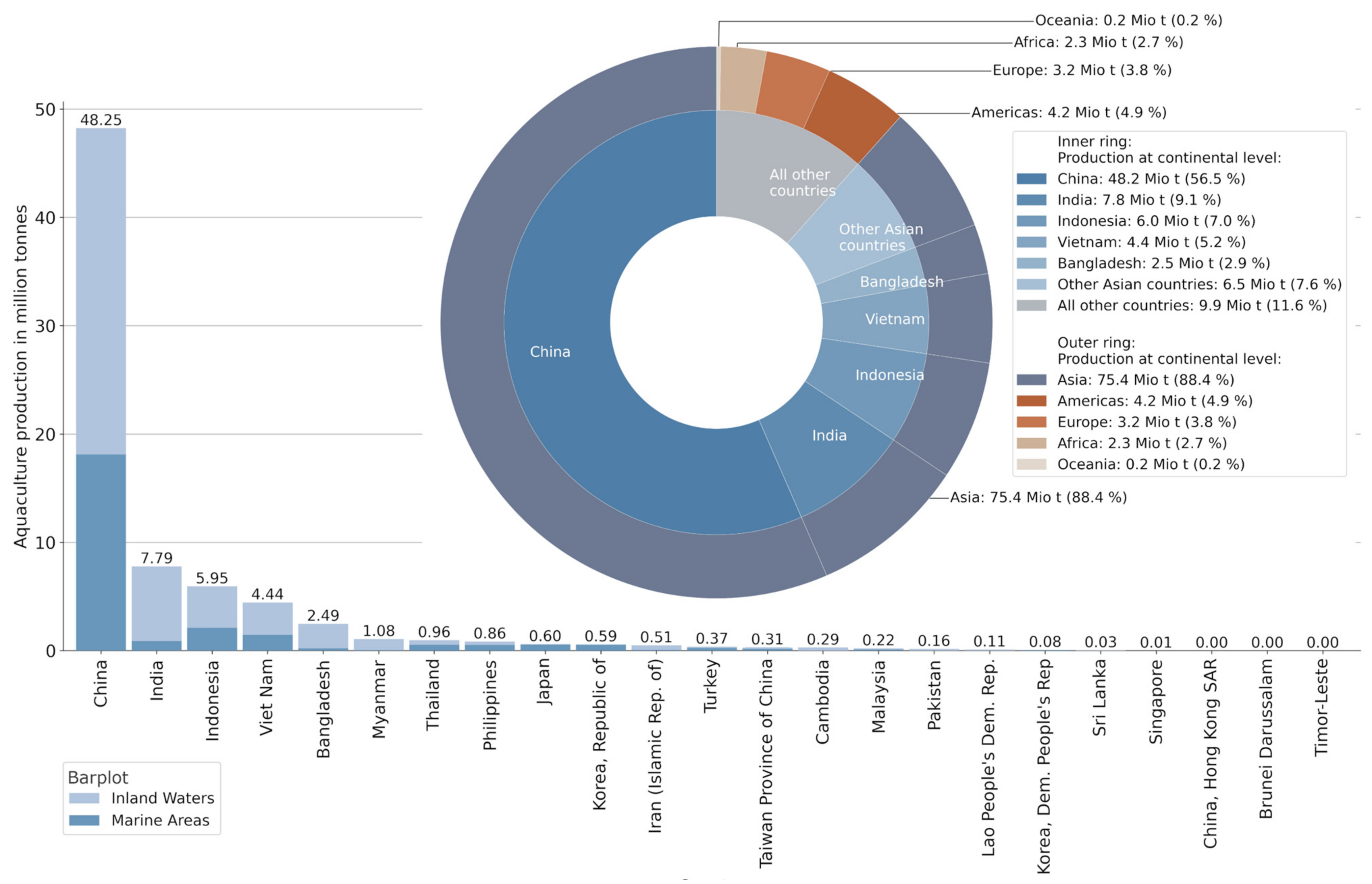
At the continental and national levels, there are very large regional differences in aquaculture production. The five largest aquaculture-producing countries contribute to more than 80 percent of the global volume and all come from Asia: China (48.2 million t), India (7.8 million t), Indonesia (6.0 million t), Vietnam (4.4 million t), and Bangladesh (2.5 million t) (see Figure 2). In 2019, China accounted for more than half (56 percent) of the global aquaculture production, underlining its dominant role in the aquaculture sector in recent years. In Asia, aquaculture mainly takes place in closed, land-based pond systems in inland waters (see Figure 2) and ranges from extensive smallholder pond management to commercial, industrialized pond farms with advanced feeding technologies [17,18]. Satellite remote sensing enables large-scale, area-wide, and routine monitoring of bodies of water and anthropogenic activities in coastal regions [19,20] and is a suitable tool for developing geographic information products on a national, regional, or global level. As a result of the rapid global growth of aquaculture in recent years, the spatial recording and mapping of aquaculture in the coastal regions and the collection of relevant environmental data on the effects of aquaculture on natural ecosystems and their spatial and temporal changes represent a focus in coastal research. In this regard, geospatial information on aquaculture can support the management of this growing food sector for the sustainable development of coastal ecosystems, resources, and human health.

1.2. Extracting Aquaculture Using Earth Observation

Only high-resolution imagery enables the detection of even fine linear structural details of small-scale pond aquaculture objects with a size of less than 1 hectare. On the one hand, a large number of Earth observation satellites orbiting our planet with passive optical and active radar instruments with high spatial resolution are suitable for the detection and mapping of aquaculture areas, but many have limited temporal and spatial coverage. On the other hand, the object detection of pond aquaculture requires temporarily dense time series in order to distinguish ponds from temporarily flooded areas (e.g., wetlands); this cannot be clearly differentiated with mono-temporal acquisitions. Access to data from high-resolution, continuous-monitoring missions such as Landsat or the European Sentinel-1 and -2 enables the processing and analysis of long-term time series [21]. However, cloud cover limits seamless data acquisition and data availability with passive satellite sensors and makes it difficult to identify aquacultures with multispectral optical sensors [22,23,24,25,26] as a result of the lack of available data in cloud-prone regions. Active radar sensors emit electromagnetic waves in the longer microwave ranges, which are hardly influenced by the atmosphere and thus enable weather-independent mapping of the Earth’s surface [19]. Therefore, satellite-based SAR data has relevant advantages for mapping aquaculture in coastal regions regularly covered by clouds. The Sentinel-1 mission of the Copernicus program with the high-resolution Sentinel-1A and -1B satellites (including its successors Sentinel-1C/D, scheduled to be launched in 2022) is definitely a game changer: it is the first SAR-C-Band mission with open archive, providing free access to a global and temporally dense data coverage that is growing continuously (Approx. 10 terabytes per day). The access to vast amounts of freely available satellite remote sensing data and the development of high-performance and cloud computing infrastructures in recent years have significantly improved the efficiency of data processing and analysis, bringing Earth observation into a new era. This has led to the generation of new data, technologies, and products for different global-scale applications at a rapid pace [27,28].

Promising regional approaches exist for the automated extraction of land-based pond aquaculture with Landsat [29,30], Sentinel-2 [31], and Sentinel-1 data [32,33,34,35,36]. However, there is no satellite-derived mapping for land-based pond aquaculture on a continental or global scale. A satellite-based quantitative assessment of relevant geoinformation on the spatial extent, distribution, and dynamics of pond aquaculture is essential for sustainable development, and management of aquaculture in coastal Asia is of utmost importance for global food security. Therefore, it is of particular interest to monitor and collect aquaculture and provide appropriate information that can be used for research in the fields of coastal environmental change, hydrology, and oceanography, among others. The main goals of this study are therefore the development of a methodology for the automatic, continental-scale mapping of coastal pond aquaculture for the entirety of Asia based on satellite remote sensing data, as well as the assessment and analysis of aquaculture areas at national and subnational level.

2. Study Region

In this study, we focus on the coastal zone of South Asia, Southeast Asia, and East Asia, which extends over 22 Asian countries and comprises a total coastline of 300,000 km (see Figure 3 and

Table 1. Overview of all countries that belong to the study region: coastal zone of Asia (CZA).

Country	ISO 3166-1 Alpha-3 Code	Coastline Length a [km]	Land Area b [km²]	Coastline a/ Land Area a Ratio [m/km2]	Total Population (TP) c [in Mio]	Population in the Coastal Zone (PCZA) d [in Mio]	Share of PCZA in Relation to TP [in %]
Indonesia	IDN	97,680	1,878,758	51.99	267.67	250.32	93.5
Philippines	PHL	34,541	293,319	117.76	106.65	96.78	90.7
China	CHN	34,362	9,371,977	3.67	1459.38	429.65	29.4
Japan	JPN	30,725	372,424	82.50	127.20	121.38	95.4
Myanmar	MMR	18,008	662,913	27.16	53.71	28.52	53.1
Republic of Korea	KOR	14,930	96,857	154.14	51.17	48.40	94.6
India	IND	13,166	3,150,820	4.18	1352.64	386.57	28.6
Malaysia	MYS	12,465	327,849	38.02	31.53	29.73	94.3
Thailand	THA	8182	514,480	15.90	69.43	39.09	56.3
Vietnam	VNM	6217	328,898	18.90	95.55	87.09	91.1
Iran	IRN	5858	1,622,136	3.61	81.80	10.48	12.8
Pakistan	PAK	4936	872,877	5.65	212.23	24.27	11.4
Dem. People’s Rep. Korea	PRK	4896	121,458	40.31	25.55	23.71	92.8
Sri Lanka	LKA	3930	66,288	59.29	21.23	20.58	96.9
Taiwan	TWN	2863	36,207	79.07	23.73	23.06	97.2
Bangladesh	BGD	2735	137,208	19.93	161.38	82.94	51.4
Cambodia	KHM	1430	181,058	7.90	16.25	10.91	67.1
Hong Kong SAR	HKG	1101	1038	1060.56	7.37	5.93	80.5
Timor-Leste	TLS	803	15,083	53.24	1.27	1.17	92.1
Singapore	SGP	490	511	959.73	5.76	5.44	94.4
Brunei Darussalam	BRN	298	5713	52.16	0.43	0.43	100.0
Macao SAR	MAC	89	29	3068.01	0.63	0.40	63.5
ROI total (22 countries)		299,705	20,057,900	Ø 269.26	4173	1726	41.4
South Asia (SA)		30,625	5,849,329	Ø 18.53	1829	524.84	28.7
Southeast Asia Mainland (SEAL)		38,474	1,819,271	Ø 176.86	267	194.76	73.1
Southeast Asia Maritime (SEAM)		141,640	2,389,311	Ø 63.50	383	354.71	92.7
East Asia (EA)		38,415	9,409,251	Ø 1,052.83	1491	459.04	30.8
Northeast Asia (NEA)		50,551	590,739	Ø 92.32	204	193.49	94.9

ROI: Region of interest (ROI) refers to all Asian countries, which cover the coastal zone of Asia (CZA); see Section 2. ^Ø —Average value; ^a—Coastline length calculated from vector data on administrative areas from the GADM [38] dataset; ^b—Land area calculated from the free Natural Earth dataset (accessible via naturalearthdata.com); ^c—Population data source: FAOSTAT; ^d—European Commission, Joint Research Centre (JRC) (2015): GHS-POP R2015A-GHS population grid, derived from GPW4 [39].

). We defined a coastal zone of Asia (CZA) by calculating a 200-km buffer—landwards and seawards—from a detailed coastline of Asia. Efficient coastal sections were designed in this study in order to enable processing of large satellite data time series for the entire coastal zone of Asia. For this purpose, the 200-km-wide coastal buffer was subdivided into 261 coastal parcels (see Figure 3) by calculating and digitizing lateral sections with a distance interval of 200 km coastline length.

The final coastal zone stretches from Iran in the west to Western New Guinea in the southeast and Japan in the northeast and is inhabited by more than 1.7 billion people (see Table 1), which corresponds to almost a quarter (22 percent) of the current world population. The zone represents environments with different climates, different terrains, and a variety of terrestrial and aquatic ecosystems. Rapid socio-economic development, increased urbanization, and coast-ward migration [37], however, dramatically changed the coastal regions in Asia during the last two decades. Land use changes were closely related to the expanding farming of crops (e.g., paddy rice), fish and shrimp, which are the main food source for millions of people. For a more general spatial comparison in Section 4, we also defined five macro-regions (see Figure 3 for coverage and Table 1 for country codes): South Asia (IRN, PAK, IND, LKA, BGD), Southeast Asia Mainland (MYR, THA, KHM, VNM, West-MYS, SGP), Southeast Asia Maritime (East-MYS, IDN, PHL, BRN, TLS), East Asia (CHN, MAC, HKG, TWN), and Northeast Asia (PRK, KOR, JPN).

The coastal zone in South, East, and Southeast Asia with its variety of lagoons, estuaries, river deltas, and abundant water resources provides ideal conditions for breeding fish and crustaceans. Above all, the low-lying, flat-topography areas along the coastal regions fostered the rapid growth of pond aquaculture. As a result, the fertile and often densely populated coastal regions in Asia have experienced large-scale changes of land use and shifts in farming systems [8,40], primarily through the expansion and intensification of agriculture and land-based aquaculture, which provide the staple foods for the majority of the coastal population. At the same time, the coastal zone is one of the most threatened regions in the context of global environmental changes and global climate change effects, such as increased frequency of weather extremes (floods, droughts, and storms) and salinization [9,16,41,42]. Table 1 shows the main characteristics of the respective countries that cover the coastal study region. The large island state Indonesia with its coasts on Borneo, Sumatra, Java, Sulawesi and New Guinea has the longest coastline of all Asian countries, with a total length of 97,680 km. The total population of the coastal zone defined in this study makes up 41 percent of the total population of the countries that belong to this zone. More than half of the coastal countries (12 out of 22) have from 90 to 100 percent of their total population within 200 km of the coast (see Table 1).

3. Data and Methods

Land-based pond aquaculture objects can be identified and distinguished from other artificial or natural water bodies (such as rivers, lakes, reservoirs) with radar satellite data on the basis of different backscatter intensities on their structural components (low backscatter on smooth water surface, strong backscatter on surrounding dams, dikes) in combination with size and shape features. The data and methodological workflow for the mapping of coastal aquaculture in this study is based in parts on the processing steps published in [32]. The method was adapted and further developed in order to enable large-scale continental mapping: the processing of the satellite data and the segmentation and vectorization of the aquaculture objects including temporal features were carried out in the JavaScript API of the cloud computing platform Google Earth Engine (GEE). Further post-processing workflows and statistical analysis were carried out with the free and open source software QGIS and with the Python libraries pandas, geopandas, and geofeather (for more details, please see Appendix A).

3.1. Satellite Data

3.1.1. Sentinel-1 Time Series Data

For each study site in the entire Asian coastal zone, we used all available Sentinel-1 dual-polarized (VV + VH) data in Interferometric Wide-Swath Mode (IW) and Ground Range Detected High-Resolution (GRDH) format for the time period from 1 January 2019 to 31 December 2019 [43] (see

Table 2. Available Sentinel-1 IW GRDH scenes for the study region for the complete year 2019.

Sentinel-1A/B IW GRDH		Number of Scenes
		Ascending Orbit	Descending Orbit	Ascending + Descending Orbit
Quarter I 2019	1 January–31 March	2959	3168	6127
Quarter II 2019	1 April–30 June	2940	3088	6028
Quarter III 2019	1 July–30 September	3160	3229	6389
Quarter IV 2019	1 October–31 December	3144	3746	6890
Total		12,203	13,231	25,434

and Figure 4). Sentinel-1 is a twin-satellite constellation with a synthetic aperture radar instrument operating in the C-band at a frequency of 5.4 GHz. Sentinel-1A and Sentinel-1B were launched in April 2014 and April 2016, respectively, enabling continuous, high-resolution radar mapping at global coverage scale with high repetition frequency (revisit time of up to 6 days with two satellites).

IW is the default mode over land, which captures three sub-swaths using Terrain Observation with Progressive Scans SAR (TOPSAR) recording data with a 250 km swath at 5 m by 20 m spatial resolution (resampled to 10 m spacing for GRDH products). The Sentinel-1 mission provides day, night, and all-weather observation capabilities [44,45] and ensures data continuity along with the upcoming launches of the successor satellites Sentinel-1C and 1D within the next few years.

3.1.2. Sentinel-2 Time Series Data

For the entire study region, we used all available Sentinel-2 L2A Surface Reflectance data (more than 47,000), which have been acquired by its wide-swath, high-resolution sensor—the multi-spectral Imager (MSI). The L2A data accessible via the Google Earth Engine that was downloaded from the Copernicus Open Access Hub (https://scihub.copernicus.eu, accessed on 10 November 2021) and atmospherically corrected using the Sen2Cor processor [46]. The Sentinel-2 data contains 12 spectral bands ranging from the visible to the near-infrared and spatial resolution of 10 m to 60 m.

3.2. Auxilliary Data

3.2.1. DEM Data

For the identification of potential aquaculture areas (low topography, flat regions), we derived terrain information using the Shuttle Radar Topography Mission (SRTM) Digital Elevation Model (DEM) in Version 3 published by NASA JPL [47,48], which provides void-filled data with a high spatial resolution of 30 m. We used the elevation (height above sea level in meters) and slope (in decimal degree) information, which were considered as the most important parameters influencing the presence or absence of aquaculture ponds in the low-lying coastal regions, and used for topographical masking.

3.2.2. Administrative Boundary Data

Administrative boundary data was collected and processed to match statistical data and the pond aquaculture vector data (derived from Earth observation data) to geographical units. The geodatabase released by GADM provides comprehensive and detailed spatial data on administrative areas for all countries and their sub-divisions (ADM0–country level, ADM1–province level, ADM2–district level). The downloaded data was extracted from the GADM database in version 2.8 (April 2020).

3.2.3. Coastline Data

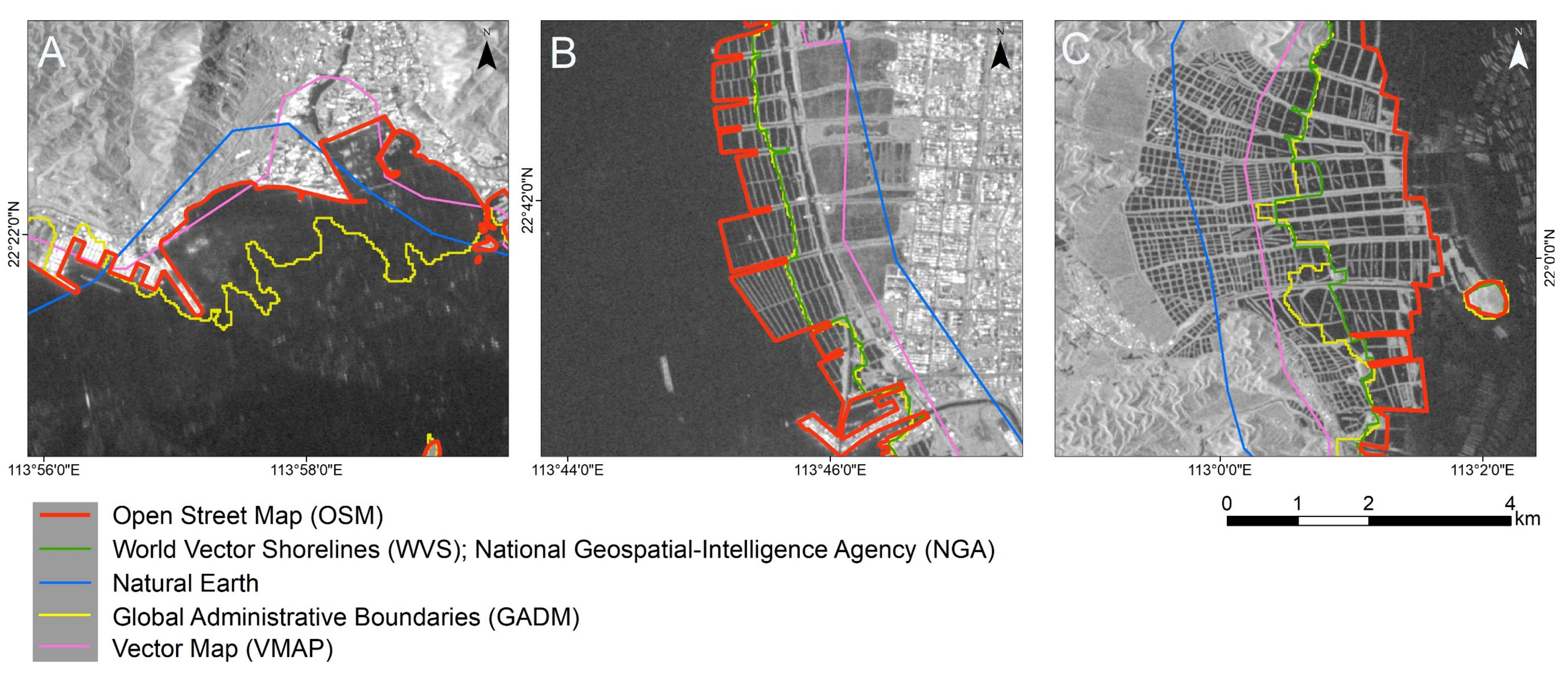
For the separation of land and ocean areas, we generated a land mask and a sea mask for the entire coastal zone of Asia on the basis of a detailed coastline dataset that represents the boundary between land and ocean areas. Accurate determination of the coastline is critical to the separation of water and land, as it determines the zone to be masked as containing potential aquaculture areas. For comparison, various global shoreline datasets from multiple sources were searched, collected, and processed to cover the entire coastal zone of Asia. The positional accuracy of all coastlines was examined for several coastal samples along the investigation areas. The Open Street Map (OSM) dataset turned out to be more detailed and up-to-date than other coastline vector datasets (see Figure 5).

3.2.4. Statistical Data

The Food and Agriculture Organization of the United Nations (FAO) publishes national catch fisheries and aquaculture statistics in their annual Yearbook of Fishery and Aquaculture Statistics [49], which are provided by national ministries and institutions. The Fisheries and Aquaculture Department of the FAO compiles and disseminates time series of fishery data, which are publicly available within its data collections on capture and aquaculture statistics. This FAO FishStat database provides these data, which are structured at a national level, providing a comprehensive overview of this sector. Aquaculture production statistics were harmonized and downloaded from the FAO Fishstat software [1], a global database with national-level production data that are submitted by FAO member countries (see

Table 3. Aquaculture production (excluding aquatic plants) for all countries in the study region and respective shares of the main aquatic product groups in 2019. Data source: [1].

Country	Total *		Fishes		Crustaceans		Mollusks
	tons	World Share (%)	tons	World Share (%)	tons	World Share (%)	tons	World Share (%)
China	48,246,255	56.54	27,086,062	48.09	5,674,350	54.14	14,579,369	83.07
India	7,795,000	9.13	7,005,792	12.44	776,208	7.41	13,000	0.07
Indonesia	5,950,000	6.97	4,913,000	8.72	977,800	9.33	58,400	0.33
Vietnam	4,442,257	5.21	3,137,200	5.57	977,157	9.32	315,000	1.79
Bangladesh	2,488,600	2.92	2,342,768	4.16	145,832	1.39	/	/
Myanmar	1,082,141	1.27	1,019,886	1.81	62,255	0.59	/	/
Thailand	964,266	1.13	431,423	0.77	384,567	3.67	116,135	0.66
Philippines	858,277	1.01	709,317	1.26	87,345	0.83	61,615	0.35
Japan	598,229	0.70	278,429	0.49	1400	0.01	305,500	1.74
Republic of Korea	593,586	0.70	112,124	0.20	7952	0.08	442,046	2.52
Iran	505,000	0.59	449,950	0.80	55,050	0.53	/	/
Cambodia	305,408	0.36	291,738	0.52	1590	0.02	11,900	0.07
Taiwan	291,499	0.34	197,516	0.35	17,621	0.17	73,500	0.42
Malaysia	224,171	0.26	153,033	0.27	53,909	0.51	16,608	0.09
Pakistan	160,744	0.19	160,438	0.28	306	0.00	/	/
Dem. People’s Rep. Korea	76,560	0.09	13,995	0.02	/	/	62,400	0.36
Sri Lanka	33,841	0.04	27,448	0.05	6098	0.06	27	0.00
Singapore	5831	0.01	4708	0.01	195	0.00	15	0.00
Hong Kong SAR	3787	0.00	3167	0.01	/	/	620	0.00
Macao SAR	1500	0.00	1020	0.00	440	0.00	40	0.00
Brunei Darussalam	933	0.00	341	0.00	592	0.01	2	0.00
Timor-Leste	120	0.00	119	0.00	1	0.00	/	/
ROI total (22 countries)	74,628,006	87.45	48,339,474	85.82	9,230,669	88.07	16,056,177	91.49
Asia total	75,435,608	88.40	49,082,188	87.14	9,321,341	88.93	16,060,694	91.51
World total	85,335,990	100.00	56,327,079	100.00	10,481,319	100.00	17,550,576	100.00

ROI: Region of interest (ROI) refers to all Asian countries, which cover the coastal zone of Asia (CZA); see Section 2. * excluding aquatic plants; Note: / represents lack of available data or the production volume is regarded as negligibly low.

).

3.3. Satellite Data Processing

In this study, we utilized all available Sentinel-1 IW GRDH and Sentinel-2 L2A data from 1 January 2019 to 31 December 2019, provided as an analysis-ready data (ARD) cube within the satellite imagery archive by the Google Earth Engine team [28]. The global datasets of the twin-satellite missions Sentinel-1 and Sentinel-2 have been available since October 2014 (Sentinel-1A) and June 2015 (Sentinel-2A), respectively. Based on experience from a previous study [32] on the use of Sentinel-1 SAR data for the mapping of aquaculture for four river deltas in Asia, the multi-sensor approach presented in this study has been further developed and adopted. The most significant advancement is the integration of water coverage information derived from multispectral Sentinel-2 data. Figure 6 shows all relevant processing steps of the applied workflow in this study. Processing of the satellite time series data comprises the following steps: (1) data selection and pre-processing, (2) calculation of time series metrics, and (3) object segmentation with histogram-based thresholding. These steps are described in detail in a previous publication [32] and are presented here in summarized form.

3.3.1. Preprocessing of Sentinel Time Series

For the time series calculation, we used analysis-ready archive data from the Google Earth Engine, which provides pre-processed Sentinel-1 and Sentinel-2 data. The scenes of the Sentinel-1 data cube are pre-processed to the backscatter coefficient σ0 (sigma0 or sigma nought). Preprocessing of the radar time series comprises the following steps: (1) the application of an orbit file, (2) thermal noise removal, (3) radiometric calibration, and (4) orthorectification. In order to limit the effects of look angle and orbit direction for each individual pixel, the Sentinel-1 data was filtered to the orbit direction (ascending or descending) with most observations (majority filter on each pixel). The preprocessing of the Sentinel-2 L2A data included the following steps: (1) cloud filtering (<10 percent cloudy pixel per scene) and (2) cloud masking using the QA60 bitmask band.

3.3.2. Derivation of Temporal Metrics

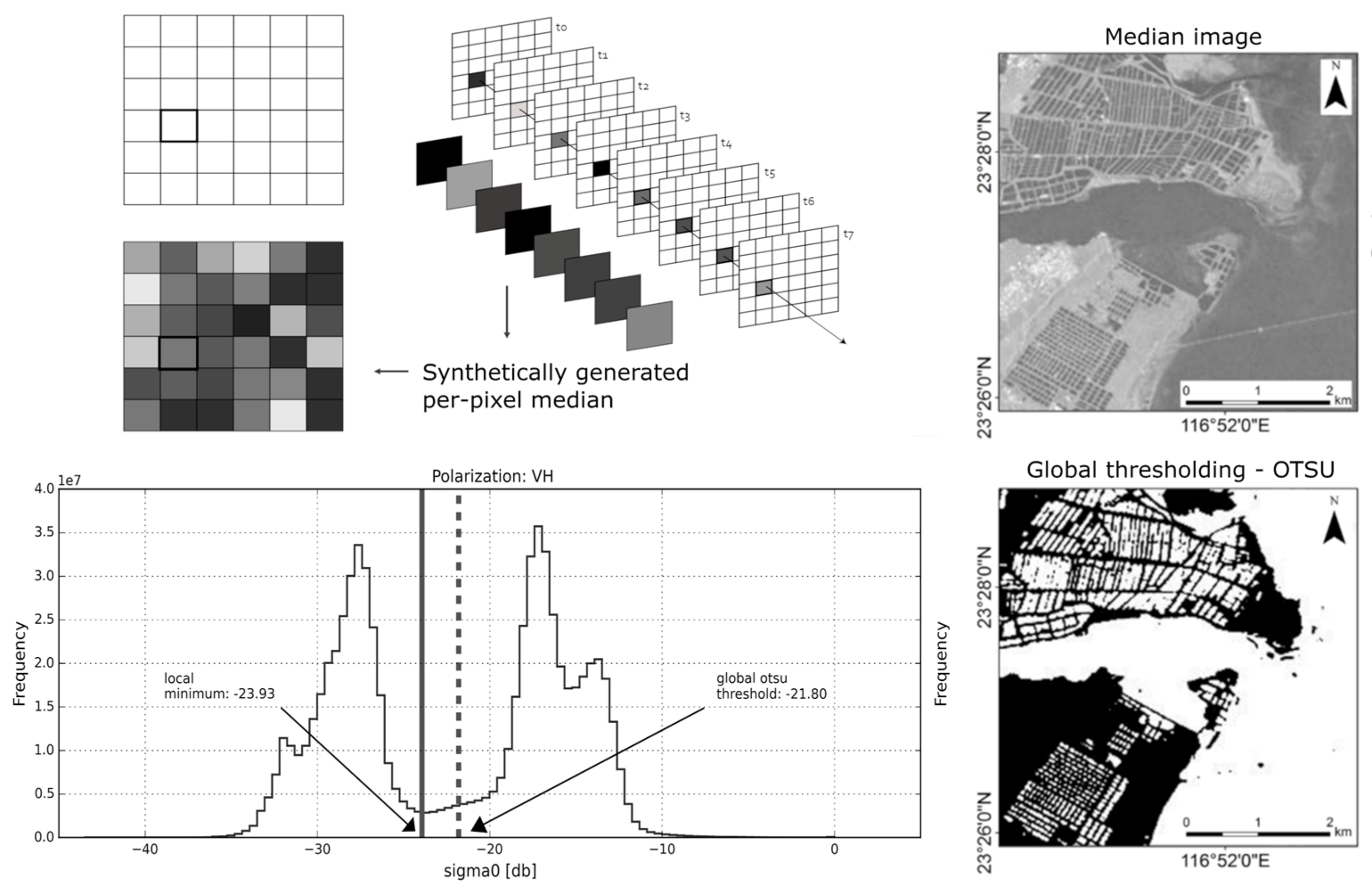
The basis for the segmentation procedure, shown in Figure 6, consists of multi-temporal metrics that have been calculated for all Sentinel-1 and Sentinel-2 scenes from 1 January to 31 December 2019. For the Sentinel-1 SAR data cube, we calculated the median; standard deviation; 10th, 25th, 50th, 75th, and 90th percentile; and standard deviation of the VH and VV polarized data. The pixel-wise median (50th percentile) is particularly suitable for identifying permanent and stable high (dams, dikes) and permanent low scatterers (smooth water surface) from the dense annual time series. A per-pixel median image was generated and used for the object-based extraction of pond aquaculture on a single-pond-unit basis. The median of all observations was selected rather than the mean to describe a single and more typical backscatter value because of the strong influence of possible extreme outliers of mean values [32,50]. By averaging over time, the temporal median image improved the appearance of narrow, elongated line structures such as dams and levees (surrounding ponds), which is very crucial for the detection and mapping of aquaculture on a single-pond level. For the optical multispectral Sentinel-2 data cube, we calculated the median of band 2 (blue), band 3 (green), band 4 (red), band 8 NIR), band 11 (SWIR), and the Normalized Difference Vegetation Index (NDWI) by Gao [51] and McFeeters [52] and the modified NDWI (MNDWI) [53].

3.3.3. Segmentation

An automatic segmentation of the median image was applied using a histogram-based thresholding algorithm by OTSU [54] that is suited for the separation of bimodal distributions [32]. OTSU’s method [54] is non-parametric, unsupervised, and used for automatic threshold selection grey-level histograms. It calculates the optimal threshold separating two classes by minimizing the weighted sum of within-class variances for an assumed bimodal histogram (see Figure 7). In a following step, the binary output image of the histogram-based thresholding of the median σ0 values at VH polarization (segments based on pixel data) was converted from raster to vector features. The resulting objects were then used to extract the following features for each pond object: temporal metric features of the satellite data (SAR features and optical features of Sentinel-1 and Sentinel-2) and topographic features (mean of the elevation and slope derived from the DEM data), which we stacked into one combined feature data cube. The object-based pond dataset was processed for each coastal parcel and downloaded in GeoJSON format automatically in a script written in the GEE JavaScript API. The final results of the 261 parcels were then merged to five macro-regions (see Section 2) instead of one single file in order to limit memory limitations on local machines and enable further processing.

On the basis of DEM-derived terrain information and coastline data, potential pond aquaculture areas were identified and extracted in order to exclude other water bodies that are most likely to be confused with aquaculture ponds, such as small mountain lakes or reservoirs located in higher latitudes. The topographical features of elevation and slope derived from the high-resolution SRTM dataset were used to generate a static mask to extract flat and low-lying coastal areas where pond aquaculture could potentially occur (see Figure 6). For this purpose, the mean elevation and mean slope values were determined from digitized pond aquaculture samples along the coastal zone of Asia to derive representative threshold values for the static mask. We defined a height of less than 50 m above sea level and slope of less than 10 percent as threshold values for generating the topographic masks (altitude mask and slope mask).

3.4. Pond Objects Filtering (Post-Processing)

In a final step, we focused on the evaluation of multiple criteria in order to improve the aquaculture mapping result and minimize the false positive rate. For this purpose, we added geometrical parameters and overlap analysis based on water features derived from the OSM dataset. All these processes are part of the post-processing workflow and have been integrated into a customized model with QGIS for automatic post-processing of the extracted aquaculture pond datasets.

3.4.1. Vector Attribute Filtering Using Geometric Features

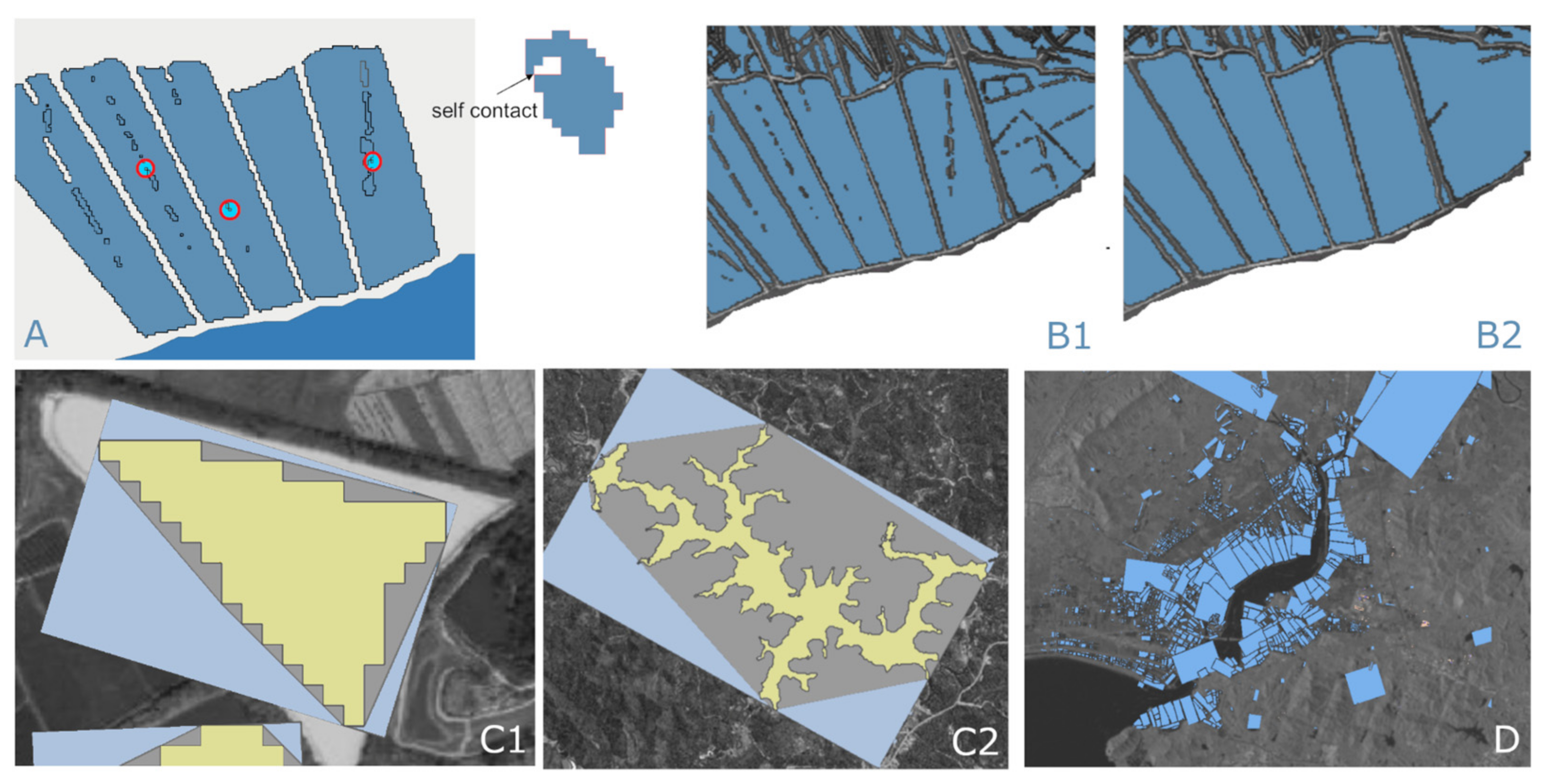
The compact shapes (mainly rectangular/circular) of aquaculture ponds are a characteristic and defining feature for the distinction between natural standing waters and managed aquaculture ponds. Without such information, the aquaculture areas, which are generally permanently covered by water, can hardly be distinguished from other (natural) water bodies. For this reason, we calculated four different geometrical parameters for the merged aquaculture pond outputs of the five Asian coastal macro-regions and added them to the mapping results. During the segmentation process, we converted the mapping results from raster to vector format. This resulted in self-contacts at the edges of some polygons, e.g., two vertices of the same polygon have the same coordinate (see Figure 8A), leading to invalid geometries. Therefore, a negative buffer at a distance of −10–6 m was calculated and applied to the pond polygon file to eliminate invalid self-contacting polygons. At the end of the post-processing, a positive buffer with the same distance was applied in order to reconstruct the original geometry of the pond polygons. Holes inside the segmented aquaculture ponds posed another challenge and influenced the perimeter length of the polygon (see Figure 8(B1)). Since the perimeter is also used for the calculation of some compactness features, existing holes needed to be filled (see Figure 8(B2)) for a proper representation of the pond area as a polygon.

To resolve these issues, the following steps were required as a preliminary process: (1) patching of holes, (2) reprojection to the global metric coordinate system (EPSG: 3857), and (3) elimination of polygon self-contact. For all aquaculture polygons we calculated the following geometric attributes, which indicate shape metrics of the pond polygon features and can be used to eliminate classification errors. The compactness, convex hull, and oriented minimum bounding box were calculated to describe the convexity, elongation, and rectangularity of a pond polygon. The ratio between area and area of the convex hull was found to be a good indicator to eliminate polygons with non-rectangular shapes. For example, lakes with dendritic shapes (see Figure 8(C2)) or rivers with curved shapes could be excluded after applying a filter of geometric attributes. We defined more than 10 test sites distributed across the study region and empirically determined threshold values based on the geometric parameters.

3.4.2. Filtering of Natural Water Bodies

As a final post-processing step, we applied an overlap analysis between the pond aquaculture mapping result and natural water body dataset. The overlap analysis on the basis of the globally available OSM dataset allows for the removal of even compact lakes and rectangular river segments (e.g., river section in between two bridges) that cannot be detected via geometrical parameters. For all countries in the study region, we acquired and merged all OSM country datasets (accessed via http://download.geofabrik.de/, accessed on 8 May 2020) and filtered for all relevant water data (OSM keys “natural = water” and “landuse = reservoir”, waterway = *), which are available in polygon (water) and polyline (waterway) format. The resulting OSM overlap percentage with the aquaculture pond dataset was calculated, and all polygons with more than 20 percent coverage were excluded.

3.5. Accuracy Assessment

A reference dataset including two classes—aquaculture ponds (AP) and non-aquaculture ponds (Non-AP)—was created for the entire coastal study region. We randomly distributed a total of 7500 sample points per class along the coastal buffer using a stratified sampling scheme [55] to adequately represent the amount of detected pond aquaculture area between different coastal regions. In order to include a statistically sound data basis for the validation, the proportion of the AP class for each of the 261 coastal parcels (see definition of parcels in Section 2) was calculated. The 7500 AP sample points and 7500 Non-AP sample points were distributed according to the parcels’ shares of the total aquaculture area. Reference data was derived from several remote sensing experts who assigned a class to each sample point (AP or Non-AP) for the entire coastal zone based on optical satellite imagery. The acquisition of very high-resolution optical data is clearly limited, since continuous coverage of the large areal extent of the continental-scale study region with a total coastline length of approximately 300,000 km (see Table 2) is too cost-intensive. For this reason, we used very high-resolution optical data provided via Google Earth imagery. Since these data are globally available, a comprehensive validation database could be provided in order to assess the accuracy of the mapping results even for very remote coastal sites and areas. Finally, we calculated a confusion matrix including performance measures such as the overall, producer’s, and user’s accuracy for the entire study region as well as for the five macro-regions (see

Table 4. Accuracy assessment for the two classes of aquaculture and non-aquaculture for the entire coastal study region. Producer’s accuracy (PA), user’s accuracy (UA), and overall accuracy (OA).

Classification	Reference
		AP	Non-AP	Sum	UA
	Aquaculture Ponds (AP)	6483	1017	7500	86.44
	Non-Aquaculture Ponds (Non-AP)	198	7302	7500	97.36
	Sum	6681	8319	15,000
	PA	97.04	87.77		91.90	OA

).

3.6. Geospatial and Statistical Data Analysis

For statistical analysis of the post-processed aquaculture pond objects, we calculated summary statistics and spatial statistics using the pandas library in Python. The post-processed pond vector files include more than 30 features and are large datasets with more than 10 GB data. In order to bypass memory limitations and enable faster data processing, we transferred the datasets for intermediate data storage into the geofeather format (https://pypi.org/project/geofeather/, accessed on 29 October 2021), which supports pandas data frames and enables faster import and export of larger geospatial files. To characterize national- and sub-national-level statistics of aquaculture pond objects such as amount, area, shape, and size features, we merged the pond object vector file with the administrative areas at three different administrative levels (GADM0, GADM1, GADM2, see Section 3.2.2).

4. Results

4.1. Aquaculture Mapping Results for Coastal Asia

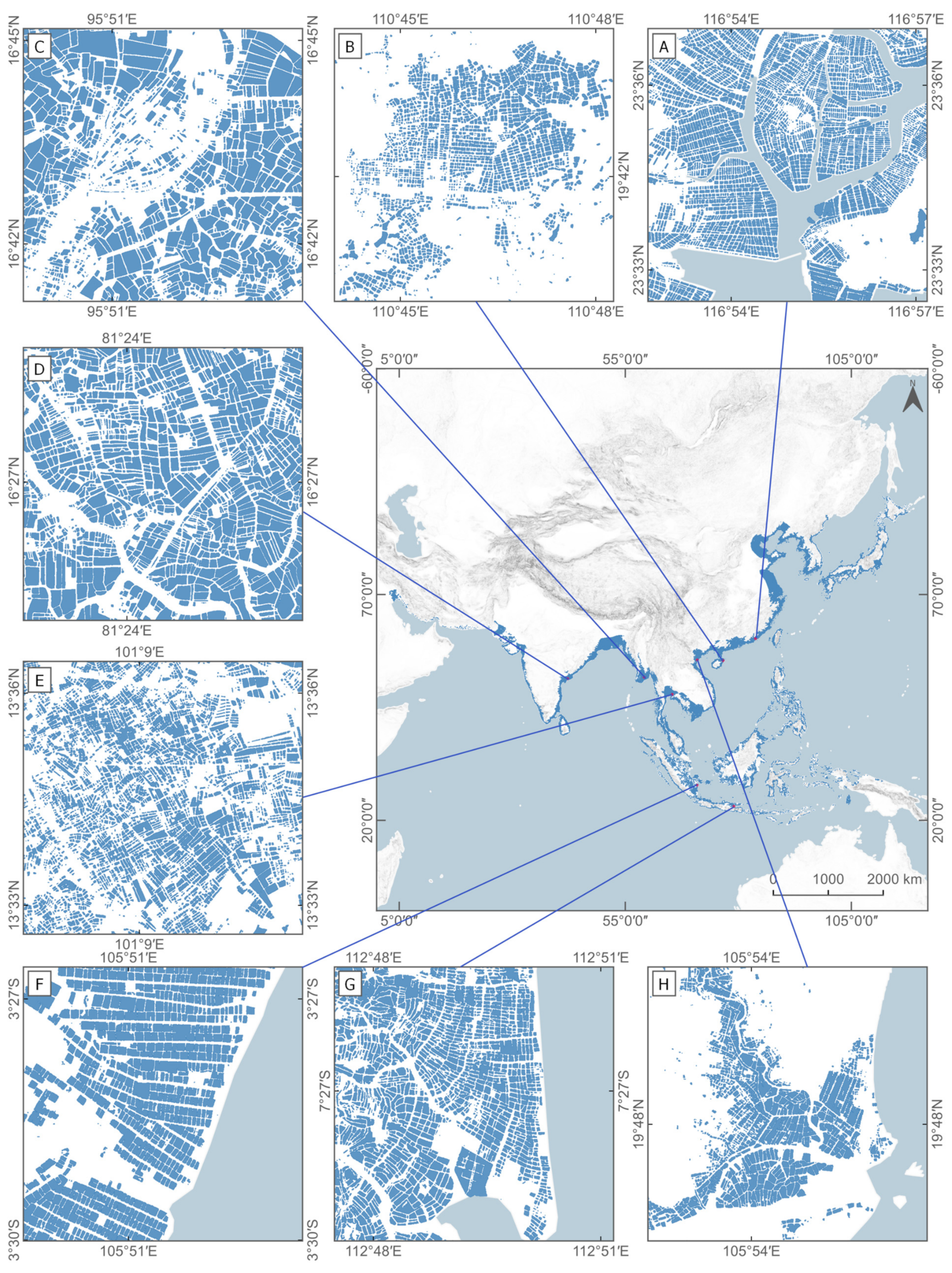
The results of the object-based pond aquaculture area extraction for the entire coastal zone and selected coastal study areas are presented in Figure 9. Due to the small object size of the ponds, it is difficult to display the entire object-based mapping result for the complete study area. Therefore, we illustrate some exemplary coastal spots located along the shoreline of Asia, with the respective mapped aquaculture objects illustrated in blue color (see Figure 9). We calculated the accuracies for the two classes (aquaculture pond and non-aquaculture pond) for the entire coastal study region. In order to quantify the agreement between the mapping result and the reference data set, the user and producer (UA and PA) and the overall accuracy (OA) as defined in [55] were computed (see Table 4). The aquaculture ponds in the coastal zone were mapped with a mean overall accuracy of 91.90 percent. In more detail, the overall accuracies per macro-region range from 92.69 percent in East Asia to 84.31 percent in Northeast Asia.

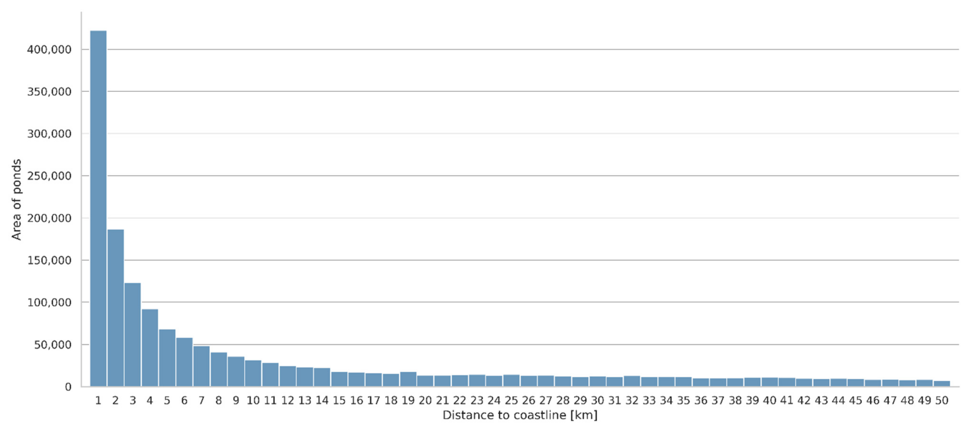
The bar plot in Figure 10 shows that the highest amount of aquaculture pond area is concentrated in close proximity along the coastline of Asia (15 km distance to the coastline) of the respective study area. The total area of the mapped aquaculture ponds within the 200 km coastal buffer zone in Asia accounts for over 2 million ha (2,000,852 ha). More than one-fifth (21 percent) of the total pond area is located within 1 km distance from the coastline, and 45 percent can be found within 5 km distance from the coastline. This indicates that pond aquaculture is clearly concentrated in close proximity to the shores.

4.2. National Statistical Analysis

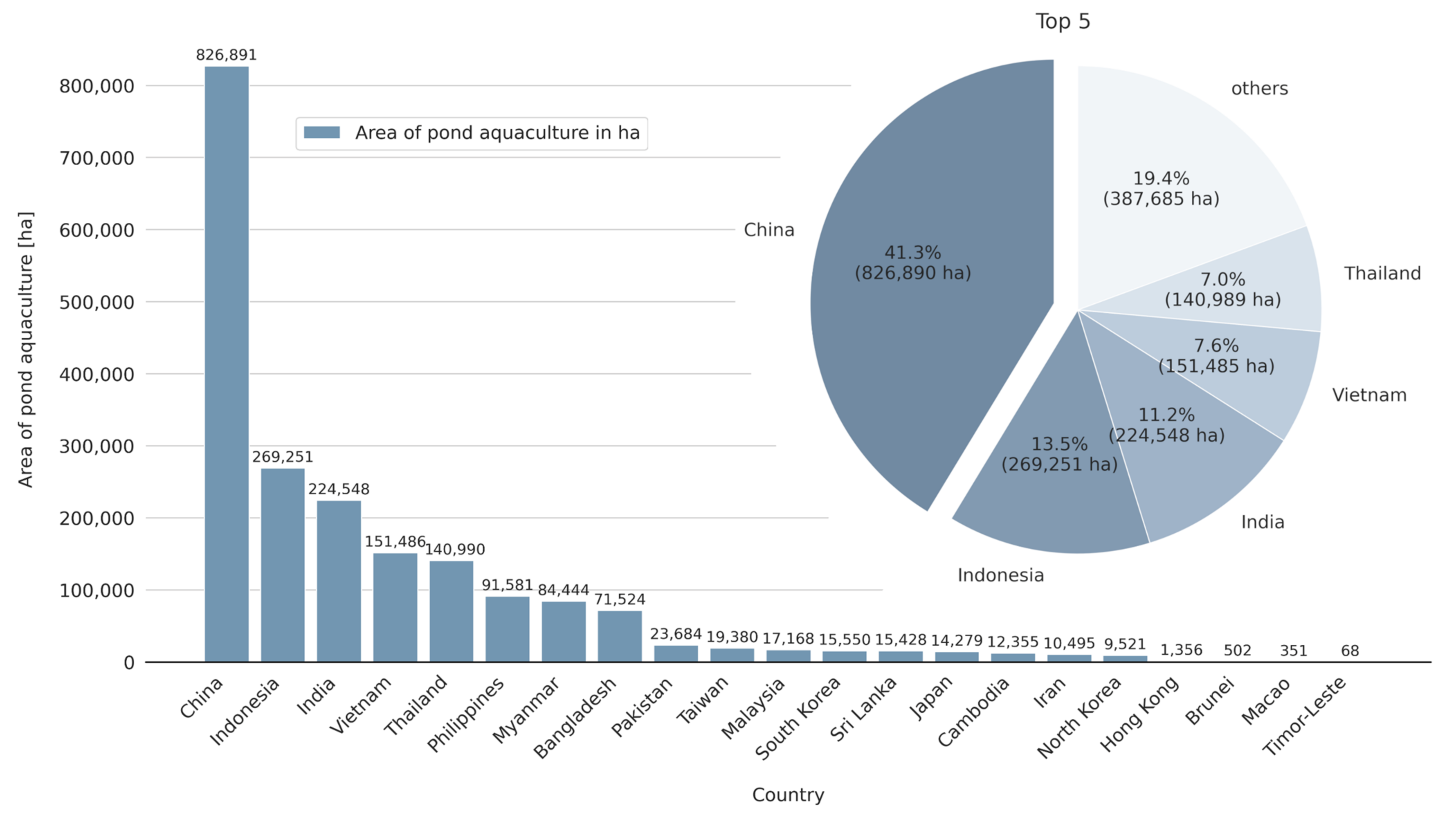
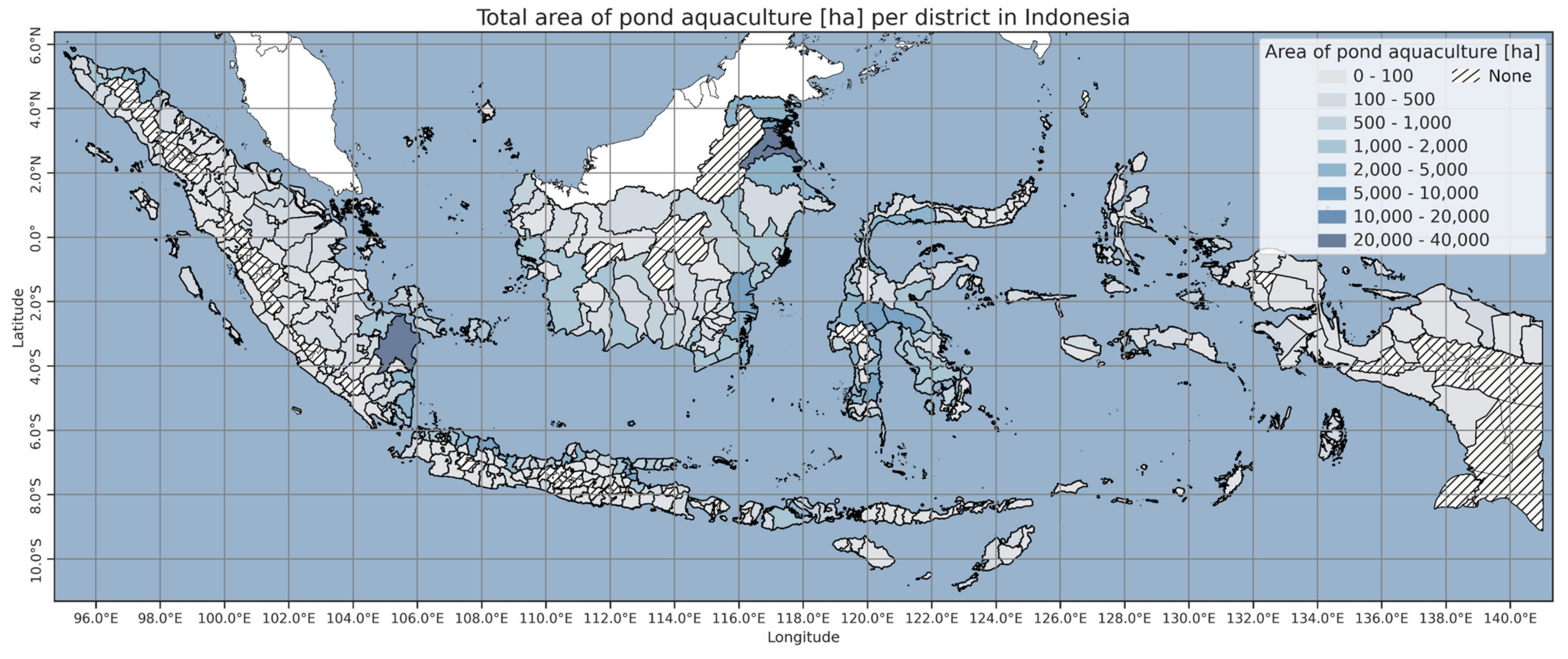
For each country, we summarize the total area of the mapped coastal pond aquaculture at national level (see Figure 11, GADM level 0), at state/province/equivalent level (GADM level 1), and district/county/equivalent level (GADM level 2). Statistics on annual aquaculture production are provided by the FAO and are listed individually for all countries. Sub-national production data are partially available for individual countries (e.g., China), but these are not available in standardized form nor accessible via a central platform for all countries at a global level. However, data at the national level may not be suitable nor relevant enough to describe regional distribution of coastal aquaculture. For this reason, we calculated coastal pond area distribution also at the sub-national administrative units to derive statistical information at the regional level. In Figure 12, we illustrate the distribution of pond area at district level for the island state of Indonesia.

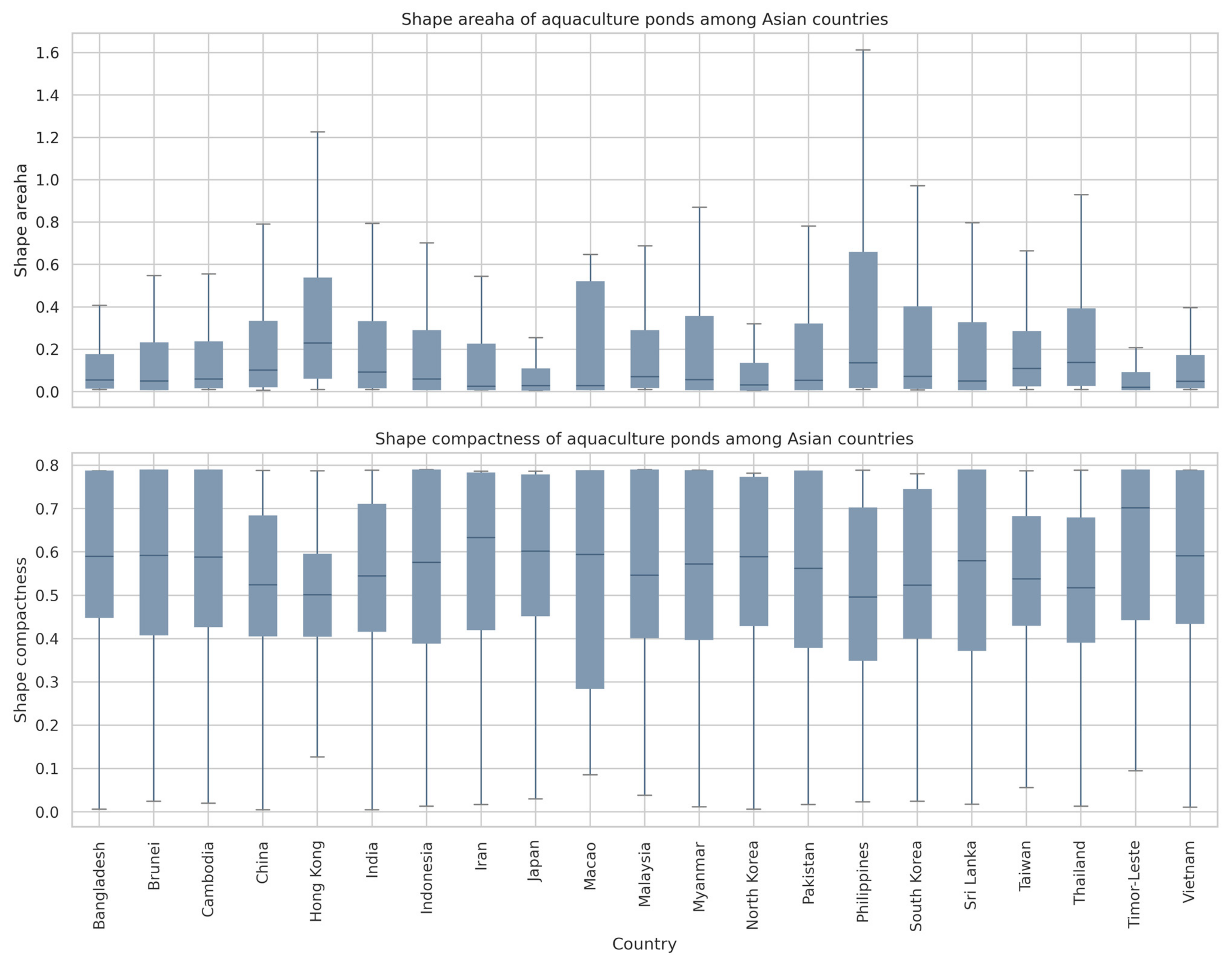
The counting and measuring of the shapes of the mapped aquaculture pond objects provides essential information to quantitatively describe the composition of shapes among different regions and countries and to recognize and describe patterns. Therefore, we analyzed various pond-specific topographic and geometric features (Figure 13) and calculated, for example, the average size and mean compactness (Figure 14) of the mapped aquaculture for each country in the study region.

For the five countries with the highest shares of mapped aquaculture area, we computed scatterplots of the elevation and distance of all ponds and found that there are different spatial patterns (Figure 13A). In China, aquaculture areas seem to be well distributed within a 150 km distance to the shorelines, while in Indonesia (and to a lesser extent also in Vietnam and India) the ponds are more concentrated within a 10–20 km distance from the coast. The reason for this could be the specific topography of the main islands of the archipelagic country Indonesia, which are characterized by volcanic mountains that slope down to the coastal plains.

4.3. Hotspot Analysis

To enable a viable representation of the results for the entire study region, the areas of the single-object pond features were aggregated to a hexagonal grid. In Figure 15, areas with high aquaculture density in the hexagon plots can be identified by blueish colors and are mainly concentrated in the greater delta regions of the Krishna River (IND), Godavari River (IND), Ganges River (BGD), Irrawaddy River (MMR), Chao Phraya River (THA), Mekong River (VNM), Pearl River (CHN), Yangtze River (CHN), and Yellow River (CHN). More hotspot regions are located in the southeast of Sumatra (IDN), along the northern coast of Java (IDN). The highest densities of pond aquaculture are concentrated in the largest aquaculture shares, which can be found along the shorelines of the coastal Chinese provinces of Hainan, Guangdong, Fujian, Zhejiang, Jiangsu, Shandong, Hebei, and Liaoning.

5. Discussion

The C-Band SAR imaging constellation of the European Sentinel-1 mission, with its continuously updated time series of all-weather high-resolution satellite imagery, is unique in radar remote sensing, representing one of the most significant data sources in Earth observation. The spatial and temporal resolution of the Sentinel-1 SAR sensor meets the requirements to recognize small-scale surface structures and individual objects on the Earth’s surface. The majority of studies on pond aquaculture detection published up to now focus rather on local studies and are limited in spatial transferability to other regions. With the availability of essential time series information derived from high-spatial-resolution Sentinel-1 radar imagery in combination with Sentinel-2 optical time series information, as well as topographical and geometric features, our study has shown that we can effectively detect and map coastal aquaculture at the single-pond level for a continental scale. Since the countries in our study region are also representative of almost 90 percent of the world’s aquaculture production, this new data set provides important information in the context of global food production and food security.

The object filtering of the automatically extracted pond aquaculture objects, which were derived from satellite time series information with segmentation algorithm, has significantly enhanced our mapping results. It has been shown that post-filtering based on vector attributes in combination with natural water overlap analysis can effectively eliminate non-aquaculture polygons. The free and open access to the water-related features contained in the OSM database provided an essential data source for the overlap analysis during post-processing in order to eliminate non-aquaculture polygons that were not determined by geometrical parameters (especially rectangular river segments).

The rectangular and compact shape of aquaculture ponds is the defining feature for the differentiation between aquaculture and other natural or artificial water bodies. Due to errors in the segmentation process of aquaculture ponds and varying shapes of aquaculture ponds, the determination of thresholds for the calculated shape-related features focused rather on optimally balancing the tradeoff between mapping accuracy and rule simplicity. The elimination of non-aquaculture polygons with individually adjusted threshold values for each coastal parcel or different coastal regions is too complex and could lead to a flawed distinction. Therefore, we applied global thresholds for the coastal Asian study region in order to exclude as many false positives (non-aquaculture polygons) as possible while preventing the exclusion of true aquaculture polygons at a minimum.

A key advantage of SAR imaging consists of its permanent observation capabilities, since radar waves can operate independent from weather conditions, cloud coverage, and time of day. Cloud cover is a prevailing issue in optical remote sensing in the context of aquaculture mapping, which limits the ability to derive full-area coverages of aquaculture from high-resolution commercial or non-commercial optical sensors. The sensor’s spatial resolution is an important criterion, because it influences the appearance of the pond objects’ shapes and is thus crucial for the selection of appropriate segmentation parameters. Even at the relatively high resolution of Sentinel-1 with a pixel spacing of 10 m, artificial elongated and narrow structures (such as dams) between individual aquaculture ponds may sometimes not be visible in the satellite data, which can result in connected ponds after the image segmentation. In these cases, (connected) pond agglomerations may have larger perimeters, lowering the objects’ compactness and thus impacting other shape metrics such as convex hull that rely on the perimeter. Aquaculture ponds generally have convex (e.g., rectangular) shapes, but sometimes they may be shaped to fit natural features (curves at rivers or terrain), which leads to concave pond shapes.

Apart from the challenges of identifying single-pond aquaculture units in radar imagery, it must be made clear that SAR sensors have clear benefits over optical remote sensing instruments for continuous mapping and monitoring of aquaculture in the coastal zone. The Copernicus Sentinel satellite missions offer free access to continuous, timely, and routine Earth observation data and thus offer enormous potential for large-scale and even global assessment of coastal aquaculture. Therefore, on the one hand, our approach for continental-scale mapping benefits from scalability through the use of the open data archives of the Sentinel-1 and Sentinel-2 satellites. These provide dense and large volumes of radar and optical imagery that can be accessed, for example, via the Google Earth Engine in preprocessed and analysis-ready data format. In our study, we make use of the analysis capabilities of Google’s cloud-based computing platform to process a full annual time series of wide-swath, high-spatial-resolution SAR and optical satellite data for coastal Asia. On the other hand, the post-processing, including the statistical analysis in our study, is based on open software, tools (e.g., python packages, QGIS, GDAL libraries), and auxiliary data (e.g., FAO fishstats, Open Street Map). As a result, the workflow presented could also be adopted and integrated into other cloud computing platforms or frameworks. For the first time, satellite remote sensing was used for the comprehensive assessment of coastal pond aquaculture at continental scale for the entire coastal zone of Asia. The method presented in this study has three major advantages:

(1)

a key feature of the novel, continental-scale mapping approach is the use of free and open remote sensing data; the launches of Sentinel-1C and 1D will provide data continuity and satellite-based high-resolution SAR data and enable continuous monitoring over the next decade;

(2)

the application of a simple and fast segmentation algorithm and scalable processing capabilities within the cloud platform provide the capacity and ability to upscale the framework and enable global mapping of coastal pond aquaculture;

(3)

the use of open source tools and software creates the possibility of integrating other or updated pre- and post-processing toolboxes, image processing, computer vision models, or algorithms into the framework.

Information on the spatial distribution of aquaculture is necessary for spatial planners, policy makers, and ecologists in order to enable sustainable development in the coastal zone and ensure food security. Aquaculture is in conflict with other existing or foreseeable land uses, e.g., urban development, tourism, and traffic infrastructure, among others. The coastal zone provides large resources for millions of people, and sustainable management is essential for future development. Operating aquaculture facilities and the construction of new ponds for fish and shrimp farming are closely linked to freshwater management (groundwater withdrawal for pond water), waste water discharge, and other ecological challenges, such as increasing coastal erosion, land subsidence, and salinization. For this reason, there is a fundamental need for further research to investigate and analyze aquaculture and its impact on natural ecosystems at continental and global scale.

6. Conclusions

A novel continental-scale mapping approach was developed to detect and assess pond aquaculture for the entire coastal zone of Asia using multi-sensor Earth observation time series. In this study, we used all available satellite data acquired by the high-resolution C-band imaging radar mission Sentinel-1 and the multispectral Sentinel-2 mission, and we calculated time series metrics to detect pond aquaculture objects. We processed more than 25,000 Sentinel-1 dual-polarized IW GRDH images, generated a temporal median image, and applied image segmentation using histogram-based thresholding to automatically detect and extract pond aquaculture on a single-pond-unit basis. The derived object-based pond units were enriched with multispectral time series information (Sentinel-2), topographic terrain information, geometric features information, and supplementary overlap analysis with global surface water data in order to extract aquaculture ponds in potential low-lying coastal areas and separate them from other natural or artificial water bodies. More than 3.4 million aquaculture ponds with a total area of more than 2 million ha were detected and mapped for a 200-km-wide buffer zone along the shoreline of South Asia, Southeast Asia, and East Asia. Spatial analyses show that aquaculture is clearly concentrated near the coast; 45 percent of the mapped ponds are located within a radius of 5 km from the coast. For each country, we summarized the total area of the mapped coastal pond aquaculture at national level and sub-national level. China accounts for the largest share of coastal pond aquaculture: 41 percent of the total Earth-observation-derived pond aquaculture area is in China, followed by Indonesia (13 percent), India (11 percent), Vietnam (7 percent), and Thailand (7 percent). The study region covers the coastal areas of 22 Asian countries, which altogether contribute more than 87 percent to the total global annual aquaculture production, representing the world’s focus in terms of aquaculture relevance. The results show that we mapped coastal aquaculture at single-pond-level with a mean average overall accuracy of 91 percent. For the first time, satellite remote sensing was used for the comprehensive assessment of coastal aquaculture at a continental scale, covering a shoreline of more than 300,000 km.

References

1. FAO Fishery and Aquaculture Statistics. Global Aquaculture Production 1950–2019 (FishstatJ). In FAO Fisheries Division; FAO: Rome, Italy, 2021. [Google Scholar]
2. Gephart, J.A.; Golden, C.D.; Asche, F.; Belton, B.; Brugere, C.; Froehlich, H.E.; Fry, J.P.; Halpern, B.S.; Hicks, C.C.; Jones, R.C.; et al. Scenarios for Global Aquaculture and Its Role in Human Nutrition. Rev. Fish. Sci. Aquac. 2021, 29, 122–138. [Google Scholar] [CrossRef]
3. Thilsted, S.H.; Thorne-Lyman, A.; Webb, P.; Bogard, J.R.; Subasinghe, R.; Phillips, M.J.; Allison, E.H. Sustaining Healthy Diets: The Role of Capture Fisheries and Aquaculture for Improving Nutrition in the Post-2015 Era. Food Policy 2016, 61, 126–131. [Google Scholar] [CrossRef] [Green Version]
4. Blanchard, J.L.; Watson, R.A.; Fulton, E.A.; Cottrell, R.S.; Nash, K.L.; Bryndum-Buchholz, A.; Büchner, M.; Carozza, D.A.; Cheung, W.W.L.; Elliott, J.; et al. Linked Sustainability Challenges and Trade-Offs among Fisheries, Aquaculture and Agriculture. Nat. Ecol. Evol. 2017, 1, 1240–1249. [Google Scholar] [CrossRef]
5. Belton, B.; Thilsted, S.H. Fisheries in Transition: Food and Nutrition Security Implications for the Global South. Glob. Food Secur. 2014, 3, 59–66. [Google Scholar] [CrossRef] [Green Version]
6. Fiedler, J.L.; Lividini, K.; Drummond, E.; Thilsted, S.H. Strengthening the Contribution of Aquaculture to Food and Nutrition Security: The Potential of a Vitamin A-Rich, Small Fish in Bangladesh. Aquaculture 2016, 452, 291–303. [Google Scholar] [CrossRef] [Green Version]
7. Béné, C.; Barange, M.; Subasinghe, R.; Pinstrup-Andersen, P.; Merino, G.; Hemre, G.-I.; Williams, M. Feeding 9 Billion by 2050—Putting Fish Back on the Menu. Food Secur. 2015, 7, 261–274. [Google Scholar] [CrossRef] [Green Version]
8. Akber, M.A.; Aziz, A.A.; Lovelock, C. Major Drivers of Coastal Aquaculture Expansion in Southeast Asia. Ocean. Coast. Manag. 2020, 198, 105364. [Google Scholar] [CrossRef]
9. Ahmed, N.; Thompson, S.; Glaser, M. Global Aquaculture Productivity, Environmental Sustainability, and Climate Change Adaptability. Environ. Manag. 2019, 63, 159–172. [Google Scholar] [CrossRef] [PubMed]
10. Dauda, A.B.; Ajadi, A.; Tola-Fabunmi, A.S.; Akinwole, A.O. Waste Production in Aquaculture: Sources, Components and Managements in Different Culture Systems. Aquac. Fish. 2019, 4, 81–88. [Google Scholar] [CrossRef]
11. Ottinger, M.; Clauss, K.; Kuenzer, C. Aquaculture: Relevance, Distribution, Impacts and Spatial Assessments—A Review. Ocean. Coast. Manag. 2016, 119, 244–266. [Google Scholar] [CrossRef]
12. Newton, R.; Zhang, W.; Xian, Z.; McAdam, B.; Little, D.C. Intensification, Regulation and Diversification: The Changing Face of Inland Aquaculture in China. Ambio 2021, 50, 1739–1756. [Google Scholar] [CrossRef]
13. Hua, K.; Cobcroft, J.M.; Cole, A.; Condon, K.; Jerry, D.R.; Mangott, A.; Praeger, C.; Vucko, M.J.; Zeng, C.; Zenger, K.; et al. The Future of Aquatic Protein: Implications for Protein Sources in Aquaculture Diets. One Earth 2019, 1, 316–329. [Google Scholar] [CrossRef] [Green Version]
14. Tacon, A.G.J. Trends in Global Aquaculture and Aquafeed Production: 2000–2017. Rev. Fish. Sci. Aquac. 2020, 28, 43–56. [Google Scholar] [CrossRef]
15. Tacon, A.G.J.; Metian, M. Global Overview on the Use of Fish Meal and Fish Oil in Industrially Compounded Aquafeeds: Trends and Future Prospects. Aquaculture 2008, 285, 146–158. [Google Scholar] [CrossRef]
16. Maulu, S.; Hasimuna, O.J.; Haambiya, L.H.; Monde, C.; Musuka, C.G.; Makorwa, T.H.; Munganga, B.P.; Phiri, K.J.; Nsekanabo, J.D. Climate Change Effects on Aquaculture Production: Sustainability Implications, Mitigation, and Adaptations. Front. Sustain. Food Syst. 2021, 5, 70. [Google Scholar] [CrossRef]
17. Bostock, J.; McAndrew, B.; Richards, R.; Jauncey, K.; Telfer, T.; Lorenzen, K.; Little, D.; Ross, L.; Handisyde, N.; Gatward, I.; et al. Aquaculture: Global Status and Trends. Philos. Trans. R. Soc. Lond. B Biol. Sci. 2010, 365, 2897–2912. [Google Scholar] [CrossRef]
18. Lazard, J.; Baruthio, A.; Mathé, S.; Rey-Valette, H.; Chia, E.; Clément, O.; Aubin, J.; Morissens, P.; Mikolasek, O.; Legendre, M.; et al. Aquaculture System Diversity and Sustainable Development: Fish Farms and Their Representation. Aquat. Living Resour. 2010, 23, 187–198. [Google Scholar] [CrossRef]
19. Ottinger, M.; Kuenzer, C. Spaceborne L-Band Synthetic Aperture Radar Data for Geoscientific Analyses in Coastal Land Applications: A Review. Remote Sens. 2020, 12, 2228. [Google Scholar] [CrossRef]
20. Cherif, E.K.; Mozetič, P.; Francé, J.; Flander-Putrle, V.; Faganeli-Pucer, J.; Vodopivec, M. Comparison of In-Situ Chlorophyll-a Time Series and Sentinel-3 Ocean and Land Color Instrument Data in Slovenian National Waters (Gulf of Trieste, Adriatic Sea). Water 2021, 13, 1903. [Google Scholar] [CrossRef]
21. Kuenzer, C.; Dech, S.; Wagner, W. Remote Sensing Time Series Revealing Land Surface Dynamics: Status Quo and the Pathway Ahead. In Remote Sensing Time Series: Revealing Land Surface Dynamics; Remote Sensing and Digital Image Processing; Kuenzer, C., Dech, S., Wagner, W., Eds.; Springer: Berlin/Heidelberg, Germany, 2015; pp. 1–24. ISBN 978-3-319-15967-6. [Google Scholar]
22. Alexandridis, T.K.; Topaloglou, C.A.; Lazaridou, E.; Zalidis, G.C. The Performance of Satellite Images in Mapping Aquacultures. Ocean. Coast. Manag. 2008, 51, 638–644. [Google Scholar] [CrossRef]
23. Marini, Y.; Prayogo, T.; Hanzah, R.; Hasyim, B. Fishpond Aquaculture Inventory in Maros Regency of South Sulawesi Province. Int. J. Remote Sens. Earth Sci. 2013, 10, 25–35. [Google Scholar] [CrossRef] [Green Version]
24. Sridhar, P.N.; Surendran, A.; Ramana, I.V.; Surendran, A.; Ramana, I.V. Auto-Extraction Technique-Based Digital Classification of Saltpans and Aquaculture Plots Using Satellite Data. Int. J. Remote Sens. 2008, 29, 313–323. [Google Scholar] [CrossRef]
25. Virdis, S.G.P. An Object-Based Image Analysis Approach for Aquaculture Ponds Precise Mapping and Monitoring: A Case Study of Tam Giang-Cau Hai Lagoon, Vietnam. Environ. Monit. Assess. 2014, 186, 117–133. [Google Scholar] [CrossRef]
26. Zhang, T.; Li, Q.; Yang, X.; Zhou, C.; Su, F. Automatic Mapping Aquaculture in Coastal Zone from TM Imagery with OBIA Approach. In Proceedings of the 18th International Conference on Geoinformatics, Beijing, China, 18–20 June 2010; pp. 1–4. [Google Scholar]
27. Chi, M.; Plaza, A.; Benediktsson, J.A.; Sun, Z.; Shen, J.; Zhu, Y. Big Data for Remote Sensing: Challenges and Opportunities. Proc. IEEE 2016, 104, 2207–2219. [Google Scholar] [CrossRef]
28. Gorelick, N.; Hancher, M.; Dixon, M.; Ilyushchenko, S.; Thau, D.; Moore, R. Google Earth Engine: Planetary-Scale Geospatial Analysis for Everyone. Remote Sens. Environ. 2017, 202, 18–27. [Google Scholar] [CrossRef]
29. Duan, Y.; Li, X.; Zhang, L.; Chen, D.; Liu, S.; Ji, H. Mapping National-Scale Aquaculture Ponds Based on the Google Earth Engine in the Chinese Coastal Zone. Aquaculture 2020, 520, 734666. [Google Scholar] [CrossRef]
30. Ren, C.; Wang, Z.; Zhang, Y.; Zhang, B.; Chen, L.; Xi, Y.; Xiao, X.; Doughty, R.B.; Liu, M.; Jia, M.; et al. Rapid Expansion of Coastal Aquaculture Ponds in China from Landsat Observations during 1984–2016. Int. J. Appl. Earth Obs. Geoinf. 2019, 82, 101902. [Google Scholar] [CrossRef]
31. Xia, Z.; Guo, X.; Chen, R. Automatic Extraction of Aquaculture Ponds Based on Google Earth Engine. Ocean. Coast. Manag. 2020, 198, 105348. [Google Scholar] [CrossRef]
32. Ottinger, M.; Clauss, K.; Kuenzer, C. Large-Scale Assessment of Coastal Aquaculture Ponds with Sentinel-1 Time Series Data. Remote Sens. 2017, 9, 440. [Google Scholar] [CrossRef] [Green Version]
33. Ottinger, M.; Clauss, K.; Kuenzer, C. Opportunities and Challenges for the Estimation of Aquaculture Production Based on Earth Observation Data. Remote Sens. 2018, 10, 1076. [Google Scholar] [CrossRef] [Green Version]
34. Prasad, K.A.; Ottinger, M.; Wei, C.; Leinenkugel, P. Assessment of Coastal Aquaculture for India from Sentinel-1 SAR Time Series. Remote Sens. 2019, 11, 357. [Google Scholar] [CrossRef] [Green Version]
35. Stiller, D.; Ottinger, M.; Leinenkugel, P. Spatio-Temporal Patterns of Coastal Aquaculture Derived from Sentinel-1 Time Series Data and the Full Landsat Archive. Remote Sens. 2019, 11, 1707. [Google Scholar] [CrossRef] [Green Version]
36. Sun, Z.; Luo, J.; Yang, J.; Yu, Q.; Zhang, L.; Xue, K.; Lu, L. Nation-Scale Mapping of Coastal Aquaculture Ponds with Sentinel-1 SAR Data Using Google Earth Engine. Remote Sens. 2020, 12, 3086. [Google Scholar] [CrossRef]
37. Neumann, B.; Vafeidis, A.T.; Zimmermann, J.; Nicholls, R.J. Future Coastal Population Growth and Exposure to Sea-Level Rise and Coastal Flooding—A Global Assessment. PLoS ONE 2015, 10, e0118571. [Google Scholar] [CrossRef] [Green Version]
38. GADM Global Administrative Areas. GADM Database of Global Administrative Areas, Version 2.0. 2012. Available online: https://gadm.org (accessed on 10 November 2021).
39. European Commission. Joint Research Centre GHS-POP R2015A—GHS Population Grid; Derived from GPW4; European Commission: Brussels, Belgium, 2015. [Google Scholar]
40. Nguyen, M.T.; Renaud, F.G.; Sebesvari, Z. Drivers of Change and Adaptation Pathways of Agricultural Systems Facing Increased Salinity Intrusion in Coastal Areas of the Mekong and Red River Deltas in Vietnam. Environ. Sci. Policy 2019, 92, 331–348. [Google Scholar] [CrossRef] [Green Version]
41. Lebel, L.; Lebel, P.; Soe, K.M.; Phuong, N.T.; Navy, H.; Phousavanh, P.; Jutagate, T.; Akester, M.; Lebel, B. Aquaculture Farmers’ Perceptions of Climate-Related Risks in the Mekong Region. Reg. Environ. Chang. 2020, 20, 95. [Google Scholar] [CrossRef]
42. McGranahan, G.; Balk, D.; Anderson, B. The Rising Tide: Assessing the Risks of Climate Change and Human Settlements in Low Elevation Coastal Zones. Environ. Urban. 2007, 19, 17–37. [Google Scholar] [CrossRef]
43. ESA. Sentinel-1 User Handbook; ESA: Paris, France, 2013. [Google Scholar]
44. Torres, R.; Snoeij, P.; Geudtner, D.; Bibby, D.; Davidson, M.; Attema, E.; Potin, P.; Rommen, B.; Floury, N.; Brown, M.; et al. Remote Sensing of Environment GMES Sentinel-1 Mission. Remote Sens. Environ. 2012, 120, 9–24. [Google Scholar] [CrossRef]
45. Schubert, A.; Small, D.; Miranda, N.; Geudtner, D.; Meier, E. Sentinel-1A Product Geolocation Accuracy: Commissioning Phase Results. Remote Sens. 2015, 7, 9431–9449. [Google Scholar] [CrossRef] [Green Version]
46. Louis, J.; Pflug, B.; Main-Knorn, M.; Debaecker, V.; Mueller-Wilm, U.; Iannone, R.Q.; Giuseppe Cadau, E.; Boccia, V.; Gascon, F. Sentinel-2 Global Surface Reflectance Level-2a Product Generated with Sen2Cor. In Proceedings of the IGARSS 2019—2019 IEEE International Geoscience and Remote Sensing Symposium, Yokohama, Japan, 28 July–2 August 2019; pp. 8522–8525. [Google Scholar]
47. NASA Jet Propulsion Laboratory (JPL) NASA Shuttle Radar Topography Mission 1 Arc Second. Version 3.0; 2013. Available online: https://cmr.earthdata.nasa.gov/search/concepts/C1000000240-LPDAAC_ECS.html (accessed on 10 November 2021).
48. Farr, T.G.; Rosen, P.A.; Caro, E.; Crippen, R.; Duren, R.; Hensley, S.; Kobrick, M.; Paller, M.; Rodriguez, E.; Roth, L.; et al. The Shuttle Radar Topography Mission. Rev. Geophys. 2007, 45, 25–36. [Google Scholar] [CrossRef] [Green Version]
49. Garibaldi, L. The FAO Global Capture Production Database: A Six-Decade Effort to Catch the Trend. Mar. Policy 2012, 36, 760–768. [Google Scholar] [CrossRef]
50. Younos, T.M.A. Advances in Water Monitoring Research; Water Resources Publication: Littleton, CO, USA, 2002; p. 244. [Google Scholar]
51. Gao, B. NDWI—A Normalized Difference Water Index for Remote Sensing of Vegetation Liquid Water from Space. Remote Sens. Environ. 1996, 58, 257–266. [Google Scholar] [CrossRef]
52. McFeeters, S.K. The Use of the Normalized Difference Water Index (NDWI) in the Delineation of Open Water Features. Int. J. Remote Sens. 1996, 17, 1425–1432. [Google Scholar] [CrossRef]
53. Xu, H. Modification of Normalised Difference Water Index (NDWI) to Enhance Open Water Features in Remotely Sensed Imagery. Int. J. Remote Sens. 2006, 27, 3025–3033. [Google Scholar] [CrossRef]
54. Otsu, N. A Threshold Selection Method from Gray-Level Histograms. IEEE Trans. Syst. Man Cybern. 1979, 9, 62–66. [Google Scholar] [CrossRef] [Green Version]
55. Congalton, R.G.; Green, K. Assessing the Accuracy of Remotely Sensed Data: Principles and Practices, 2nd ed.; CRC Press: Boca Raton, FL, USA, 2008; ISBN 978-0-429-14397-7. [Google Scholar]
Figure 1. (A) Aquaculture production among continents from 1980–2019, (B) Global aquaculture production and capture fisheries production from 1980–2019, and (C) Map of aquaculture production in 2019. Data source: [1].
Remotesensing 14 00153 g001
Figure 2. Bar chart: Aquaculture production in inland waters and marine areas among Asian countries in 2019; Donut chart: Share of aquaculture production among continents and the top 5 global producers in 2019. Data source: [1].
Remotesensing 14 00153 g002
Figure 3. Map of the study region, including the five macro-regions and the coastline parcels that encompass a coastline of ~200 km in length.
Remotesensing 14 00153 g003
Figure 4. Coverage frequency of VH-polarized Sentinel-1 scenes (1 January 2019–31 December 2019) for the coastal zone of Asia acquired in ascending and descending orbit.
Remotesensing 14 00153 g004
Figure 5. Comparison of coastline datasets for three coastal sections (AC) along the shoreline in Guangdong Province, China. Background image: Median image derived from Sentinel-1 data.
Remotesensing 14 00153 g005
Figure 6. Workflow of the applied method for the mapping of coastal pond aquaculture for Asia, with following main processing blocks: preprocessing of the SAR Sentinel-1 data and optical Sentinel-2 data, generation of time series metrics, image segmentation, masking by topographic features, and object filtering based on geometrical and water features.
Remotesensing 14 00153 g006
Figure 7. Histogram-based thresholding (OTSU) on the temporally smoothed SAR time series (median image).
Remotesensing 14 00153 g007
Figure 8. (A) Self-contacting polygon edges; (B1) Holes in polygons and (B2) Patched holes; (C1,C2) Compactness parameters: yellow—water polygon; grey—convex hull of the polygon; light blue—oriented minimum bounding box; (D) Result of the minimum oriented bounding box calculated for the aquaculture pond mapping result.
Remotesensing 14 00153 g008
Figure 9. Extracted aquaculture ponds for the entire coastal zone of Asia. Coastal spots: (A) Guangdong Province, China; (B) Hainan Province, China; (C) Irrawaddy Delta, Myanmar; (D) Andhra Pradesh state, India; (E) Chachoengsao Province, Thailand; (F) Sumatra, Indonesia; (G) Java, Indonesia; (H) Red River Delta, Vietnam.
Remotesensing 14 00153 g009
Figure 10. Total area of Earth-observation-derived aquaculture ponds per kilometer distance to the coastline.
Remotesensing 14 00153 g010
Figure 11. Bar chart: Total area (ha) of the mapped pond aquaculture per country in the study; Pie chart: Share of total mapped aquaculture area (ha) among the top 5 ranking countries (in percent).
Remotesensing 14 00153 g011
Figure 12. Mapping result: total pond aquaculture area for Indonesia at district level.
Remotesensing 14 00153 g012
Figure 13. Scatterplots of elevation and distance of aquaculture categorized among different pond sizes for the top 5 Asian countries (China, Indonesia, India, Vietnam, and Bangladesh) (A); Boxplots of the area of the convex hull (B) and the ratio between the pond area and its convex hull (C) for the mapped ponds from the five defined macro-regions East Asia (EA), Northeast Asia (NEA), South Asia (SA), Southeast Asia Mainland (SEAL), and Southeast Asia Maritime (SEAM).
Remotesensing 14 00153 g013
Figure 14. Comparative boxplots of the calculated area in ha (top) and compactness (perimeter² ∗ area) of the mapped coastal aquaculture ponds for each country in the coastal study region.
Remotesensing 14 00153 g014
Figure 15. Pond aquaculture summarized into a 5 km hexagon grid vector dataset (interlocking hexagon cells with a side length of 5 km and an area of ~65 km²). Area of aquaculture ponds per hexagon (area of ponds in ha) for the entire coastal zone of Asia. Top: Overview with three subregions and corresponding coastal spots (blue boxes): (A) South Asia with a focus on the Krishna River Delta and Godavari River Delta, India; (B) Southeast Asia with a focus on Lampung Province, Sumatra, Indonesia; (C) East Asia with a focus on Qiongzhou Strait between Leizhou Peninsula and Hainan Island, China.
Remotesensing 14 00153 g015