Deep Convolutional Neural Network for Rice Density Prescription Map at Ripening Stage Using Unmanned Aerial Vehicle-Based Remotely Sensed Images

Abstract

In this paper, UAV (unmanned aerial vehicle, DJI Phantom4RTK) and YOLOv4 (You Only Look Once) target detection deep neural network methods were employed to collected mature rice images and detect rice ears to produce a rice density prescription map. The YOLOv4 model was used for rice ear quick detection of rice images captured by a UAV. The Kriging interpolation algorithm was used in ArcGIS to make rice density prescription maps. Mature rice images collected by a UAV were marked manually and used to build the training and testing datasets. The resolution of the images was 300 × 300 pixels. The batch size was 2, and the initial learning rate was 0.01, and the mean average precision (mAP) of the best trained model was 98.84%. Exceptionally, the network ability to detect rice in different health states was also studied with a mAP of 95.42% in the no infection rice images set, 98.84% in the mild infection rice images set, 94.35% in the moderate infection rice images set, and 93.36% in the severe infection rice images set. According to the severity of rice sheath blight, which can cause rice leaves to wither and turn yellow, the blighted grain percentage increased and the thousand-grain weight decreased, the rice images were divided into these four infection levels. The ability of the network model (R² = 0.844) was compared with traditional image processing segmentation methods (R² = 0.396) based on color and morphology features and machine learning image segmentation method (Support Vector Machine, SVM R² = 0.0817, and K-means R² = 0.1949) for rice ear counting. The results highlight that the CNN has excellent robustness, and can generate a wide range of rice density prescription maps.

1. Introduction

In the United Nations 2030 Agenda for Sustainable Development [1], the goals are to eradicate hunger, achieve food security, improve nutritional status, and promote sustainable development. As one of the three major food crops in the world [2], the rice-planted area is second only to wheat. Rice is the staple food of about half of the world’s population, of which nearly 90% is produced in Asia [3]. Currently, the world’s rice planting area is about 155 million hectares, and China’s rice planting area is 30,189 thousand hectares in 2018, accounting for about 20% of the world’s planting area. Ensuring stable rice production and increasing production are of great significance for eradicating hunger and protecting human rights. Studies have shown that only an average annual growth rate of rice output of about 1% can meet the consumption demand [4]. Rice planting density [5] and the application of nitrogen fertilizer are the main techniques used in the production management process, which play a decisive role in the yield of rice. Larger density differences have a greater impact on the rice population productivity and grain yield. One of the most important aspects is the differences in the utilization of temperature and light resources by groups under different planting methods [6]; a too high or too low cultivation density will affect its yield. It is difficult to increase food production to meet the growth rate of the human population. The phenomenon of excessive grain loss from harvester operation in the field is at odds to the current situation of increasing world food shortages [7,8,9]. One of the main reasons for this problem is when harvesting high-density rice, the operating parameters of the main working parts, such as threshing drum speed, cannot be adjusted in time to adapt to the changes in the feed amount, which can lead to unclean grains and even blockages. These will cause increased grain loss. Therefore, crop density prediction that can allow enough time for harvester adjustment is of great significance for reducing grain loss during harvesting [10,11,12]. The harvesting efficiency of the rice combine harvester mainly depends on the feeding amount [13]. Under the condition of stable harvester cutting width, the feeding amount is mainly determined by the harvester forward speed and the crop density [14,15,16,17,18]. Normally, adjusting the forward speed mainly depends on the operator’s experience of judging the density of crops, which is susceptible to subjective factors, and the quality of work cannot be guaranteed. When the forward speed of the harvester is too fast, the instantaneous feeding amount may exceed the load of the machine, which will cause the harvester to block and fail [19]; if the forward speed is too low, the harvester operates at a low load, resulting in decreased harvesting efficiency. Therefore, knowing the rice density before harvesting, generating a density prescription map, and attaining a suitable operating speed to ensure the stability of the feeding amount are of great significance for improving the quality of the operation.

The current combine harvester forward speed control method is mainly based on the working parameters of the main harvester components monitored by the loaded monitoring system, such as header losses of combine harvesters [20,21,22], drum speed [23], etc., which establish speed prediction equations to achieve speed control. The method of monitoring the grain loss of the combine harvester to adjust the forward speed is when the grain loss increases, the vehicle speed is automatically reduced by the control system or the driver reduces the vehicle speed according to the grain loss value displayed on the on-board screen [20]. Alternatively, the vehicle speed should be increased appropriately. To adjust the forward speed by monitoring the drum speed of the combine harvester, when the drum speed decreases (too large a feed volume causes the drum to overload and reduce the drum speed), the vehicle speed is automatically reduced by the control system or the driver reduces the vehicle speed according to the drum speed value displayed on the onboard screen [23]. Alternatively, the vehicle speed should be increased appropriately. In both methods, the operating speed of the harvester is adjusted only after the loss of grain is too large or the rotation speed of the drum is reduced. Therefore, there is hysteresis. This is likely to cause a decrease in work efficiency and even the risk of damage to the machine. Therefore, predicting the crop density in front of the operation generating rice density prescription map with geographical coordinate information can provide strong data support for the combine harvester to operate at a reasonable operating speed.

Computer vision is currently the main technical means for rice ear recognition and counting. Visible light images of rice contain the characteristics of rice ear color [24,25], texture [26], and shape. Machine learning builds a target classifier by learning these characteristics to realize rice ear target detection. Although these methods have allowed certain achievements, the extraction of manual image features is needed, which is not suitable for the uneven illumination environment and complex background in the field, which results in poor algorithm robustness and difficulty in expanding applications. Some researchers have proposed ways to reduce these effects. For example, researchers designed an unsupervised Bayesian method based on the Lab color space of field rice UAV images and a segmentation algorithm for the extraction of rice pixel regions in the late tiller stage to reduce uneven illumination [27]. Wheat image RGB-gray image, Lab-L, HSV-V color space, and the combined morphological characteristics of wheat ears were used to extract wheat ear targets [28]. Although these methods reduce the impact of uneven illumination to a certain extent, the robustness of the algorithm still does not meet the actual application conditions under complex field environments.

A fully deep convolutional neural network is currently the most effective image recognition technology [29,30], and has a wide range of uses in agricultural fields [31,32,33], such as plant identification and classification [34,35], plant disease detection [36,37,38,39,40,41], pest identification and classification [42,43,44], plant organ count [45,46], weed identification [47,48,49], and land cover classification [50]. Based on more than 40 studies on the application of deep learning in agriculture, KAMILARIS has concluded that deep learning has higher accuracy in image recognition than existing commonly used image processing technologies, such as SVM, K-means, and random forest [51]. Xiong proposed a visual detection method to detect green mangoes by a UAV [30]. Jing Zhou used unmanned aerial vehicle-based soybean imagery and a convolutional neural network to achieve yield estimation [52]. Zhou prosed a rice disease rapid detection method with FCM-KM and Faster R-CNN fusion [53]. Xiong proposed a Panicle-SEG segmentation algorithm based on simple linear iterative clustering (SLIC) super-pixel segmentation, which is trained by constructing a CNN model and combined with entropy rate super pixel optimization to realize the identification of rice ears in the field environment [47]. Yu prosed an integrated rice panicle phenotyping method with a Faster-R-CNN method on X-ray and RGB scanning images [54]. In addition to only using deep learning to solve problems, such as prediction and recognition in the agricultural field, some scholars have also combined machine learning and deep learning methods for applied research [55]. CNN has been widely used in the agricultural field, but there are few reports on the research for the production of rice density prescription maps using a deep learning method during the maturation period.

To our knowledge, there is no former study that generates rice density prescription maps with CNNs using UAV-based remote sensing data. There are two novelties of this present study.

First, by using machine learning SVM, K-means, and manual segmentation results of rice ear image to perform the regression of the number of rice ears, we found that it is not feasible to use image segmentation algorithms for rice density statistics or yield estimation in a field environment. Second, for the first time, the recognition results of deep neural networks are applied to the production of prescription maps. The objectives of this paper are to (1) examine the capability of yolov4 in estimating mature rice density using UAV rice RGB images in an end-to-end way, (2) improve the density estimation accuracy by integrating multi-scale features and investigate the spatial range for density forecasting, (3) verify that it is not feasible to predict the ear density by the method of rice ear region segmentation in the image, and (4) provide powerful data support for the automatic control of the rice combine harvester working parameters, especially the adjustment of the forward speed, because the forward speed and the density of rice in front of the harvester affect the feed volume of the harvester. Moreover, if the density of the rice in front of the operation is known in advance, the harvester will operate at a reasonable forward speed to ensure the best feed volume, which is very significant for ensuring combine harvester operation quality.

2. Materials and Methods

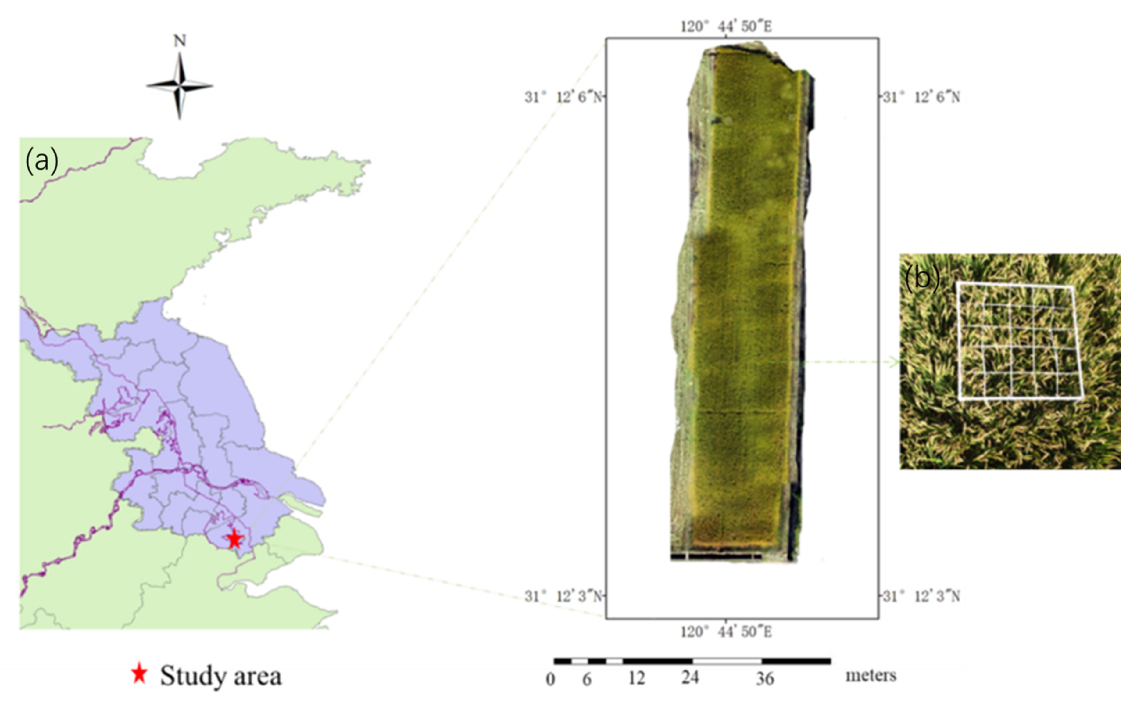
2.1. Study Area

The experimental site (31°1′52′′N, 120°31′5′′E) was located at Wujiang City, Jiangsu province, China, as shown in Figure 1. The area belongs to the subtropical monsoon oceanic climate, which has four distinct seasons and abundant rainfall. The average annual rainfall is 1100 mm, the average annual temperature is 15.7 °C, and the soil type is of paddy soil. The rice variety in the test plot was Nanjing Jinggu, which is a new generation of high-yielding japonica rice varieties developed by the excellent taste breeding team of the Institute of Food Crops, Jiangsu Academy of Agricultural Sciences.

2.2. Images Acquisition

A multi-rotor UAV (DJI Phantom 4RTK) was employed to collect mature rice images in this study between 8 November 2020 and 12 November 2020, which is equipped with a GPS sensor, inertial navigation, and 15.2 V/5870 mAh lithium battery, which can ensure that the UAV flies automatically for about 28 min on the planning route at an altitude level of 25 m above ground. The ground speed of the UAV was set at approximately 4 m/s. An RGB digital camera was mounted on the UAV to take rice images. The RGB sensor had 4864 × 3648 pixels. The short exposure time was faster than 1/8000 s, small aperture was f/2.8–f/11, and auto focus(1m-∞), which were set for cameras to avoid the blurred images.

Five flights for collecting RGB mature rice images were carried out on 8 November, 9 November, 10 November, 11 November, and 12 November (

Table 1. Details of remote sensing data acquisition.

Date	Sensor	Number of Images	Altitude (m)	Ground Resolution (mm)
08 November 2020	RGB	102	5	2.3
09 November 2020	RGB	112	5	2.3
10 November 2020	RGB	103	5	2.3
11 November 2020	RGB	107	5	2.3
12 November 2020	RGB	111	5	2.3

). During each flight, mature rice images were collected with side overlap of 70% and trajectory overlap of 80% to assure the high quality of mature rice orthoimage maps. The information about flight altitude and ground resolution during each flight is given in Table 1.

2.3. Mature Rice Image Processing

The first processing of raw mature rice image data includes two steps: (1) mature rice orthoimage map generation; (2) map geographic coordinate extraction and clipping for target area. Traditional image processing for rice ear counting is described in Section 3.2.

2.3.1. Mature Rice Orthoimage Map

PhotoScan Pro can generate high-resolution orthoimages with real coordinates and DEM models with detailed color textures. We import the images collected by the drone into this software for orthoimage generation. In the work process, according to the software prompts, we proceed to the generation of orthophotos of rice. Generating mature rice orthoimage maps has four steps: (1) raw mature rice image alignment and mosaicking; (2) sparse point cloud and mesh generation; (3) dense point cloud; and (4) orthoimage rice map export. Steps 1–4 were implemented in Agisoft Photoscan Pro software, as shown in Figure 2, which was based on the structure from motion (SfM) algorithm [56].

2.3.2. Geographic Coordinate Extraction and Clipping

First, import the orthoimage maps file into ArcGIS 10.5; then, use the resampling method to adjust the raster cell size to the same size as the sub-image size (300 pixels × 300 pixels), and finally, output a text file with latitude and longitude coordinates.

Using Visual Studio2017 and OpenCV (open source image processing library), we wrote a script to crop the generated orthoimage maps into multiple sub-images of the size 300 pixels × 300 pixels. Two hundred sub-images were selected geographically far apart as the training set, valid set, and testing set for building the target detection model.

2.4. Traditional Image Processing Technology

In this study, we used a script file written by Visual Studio with traditional image processing methods based on color, histogram equalization, Gaussian blur, and morphological characteristics to segment the ears of rice; the ear head counting was achieved by calculating the number, area, and perimeter of connected domains of the segmented image in Figure 3. As the most prevailing characteristic, color has been widely used to segment crop organ targets, such as leaves, flowers, and fruits [57]. However, the color characteristic fails to consider the influence of light noise. Many new methods were proposed to avoid the above issues. For instance, color space conversion in which the HSV color space was converted from RGB color space was employed to mitigate the influence of uneven lighting [58]. Gaussian blur was employed to mitigate the light noise by using data smoothing techniques on images. However, the results of these methods were not satisfactory.

2.5. CNN Architecture Design

Considering the phenomenon that the ears of rice at maturity are occluded by each other, the YOLOv4 [59] target detection network was employed to realize the target detection and quantity statistics of high-density rice ears.

2.5.1. YOLOv4 Network Structure

The input mature rice image data of size 300 × 300 × N was sent to the YOLOv4 network, with N = 3 the number of channels for input rice images. The architecture of the YOLOv4 used in this paper is shown in Figure 4. The network is made of three modules: backbone, neck, and prediction. The backbone contains 72 convolutional layers that contributes to CBM and CSPX. The convolutional layers extract features by filters of the size of 1 × 1 and 3 × 3. The number of filters in backbone modules was 12,606, which was inspired by Darknet53 network. The neck part adopted a classic PANet structure, which won the first place in the COCO 2017 challenge instance segmentation task and the second place in the target detection task [60]. In addition, it had an SPP that used filters with a size of 1 × 1, 5 × 5, 9 × 9, and 13 × 13. Instead of average pooling, the function used in the network pooling layers was the max pooling that adopted padding operation. After that, ‘Concat’ operation was made on feature maps, which increased the receiving range of backbone features effectively, and significantly separated the most important context features. The prediction part adopts CIOU_LOSS function (Equation (1)) that considered three important geometric factors: the overlap area, the center point distance and aspect ratio, which can solve the problem of missed detection caused by overlap, which is highly suited for the target detection of rice ears at the rice maturation stage. The three kinds of feature maps for prediction were 76 × 76, 38 × 38, and 19 × 19.

$$CIOU\_LOSS=1-CIOU=1-(IOU-\frac{{\rho }^2(b,b^{gt})}{c^2}+\alpha \nu )$$

(1)

$$\nu =\frac{4}{{\pi }^2}{\left(arctan\frac{{\omega }^{gt}}{h^{gt}}-arctan\frac{{\omega }^p}{h^p}\right)}^2$$

(2)

where IOU is intersection over union, c is the diagonal distance of the smallest closure area that can contain both the prediction box and the ground truth box, ${\rho }^2(b,b^{gt})$ means Euclidean distance between the center point of the prediction box and the ground truth box, w^gt, h^gt are the height and width of the ground truth box and w^p and h^p are the height and width of the prediction box.

2.5.2. Training and Testing

The training process is based on the stochastic gradient descent algorithm with momentum acceleration [61]. Prepare the initial weight file, label the file, and modify the configuration file for training detection model. According to the requirements of the model, put the data set under the specified path. After the training starts, the model automatically divides 90% of the data into the training set (180 images), 10% of the data as the valid set (20 images). We found another 20 new images that the model had not seen before to test the model. In the development phase, the network was trained with the training dataset and evaluated with test and valid datasets to adjust the hyperparameters for better performance. In the training process, the images dataset was divided into the mini-batches to feed into the networks. The mature rice images batch size was 1 and the model initial learning rate was 0.01 with ‘torch.optim’ package. The training was stopped when the training progress reached the upper number of iterations and the change in loss value of the deep convolutional neural network, as shown in Figure 5.

The final predicted result of density was calculated by calculate the number prediction boxes. The training and testing progress were conducted in NVIDIA GTX1650SUPER with 16GB memory using the torch deep learning toolbox.

2.6. Result Evaluation

In this study, PyCharm Community Edition 64 was used for the statistical analysis. The performance of different models was evaluated by the determination coefficient (R², Equation (3)), mean absolute percentage error (MAPE, Equation (4)), and root mean square error (RMSE, Equation (5))

$$R^2=1-{{\displaystyle {\sum }_{i=1}^n({\hat{y}}_i-y_i)}}^2/{\displaystyle {\sum }_{i=1}^n(y_i-\overline{y})}$$

(3)

$$MAPE=\frac{100}{N}{\displaystyle \sum _{i=1}^n\left|\frac{{\hat{y}}_i-y_i}{y_i}\right|}$$

(4)

$$RMSE=\sqrt{{\displaystyle \sum _{i=1}^n{({\hat{y}}_i-y_i)}^2/n}}$$

(5)

where n is the total samples in the testing set, $\overline{y}$ is the average value of the measured density of the ground-truth density of rice ears, which is the number of rice ears counted artificially on the image, and ${\widehat{y}}_i$ is the predicted rice ear density.

3. Results

3.1. Statistical Analysis of Density Data

In total, mature rice density data for 200 sites were collected from the area of the study. The collected rice density ranged from 100/m² to 350/m², with an average of 209/m² in the experimental area. To ensure the robustness of the target detection algorithm, we deliberately selected sampling points with obvious differences in rice growth; that is, sampling plots with large differences in density. Area with very low density suffered from pets and diseases because of poor management. All plots were divided into four groups according to the disease severity level (rice sheath blight) for assessing the impact of the disease severity level on yield. The four groups were healthy (no infection), mild infection, moderate infection, and severe infection. The level of disease was determined through on-site investigation by plant protection experts. Figure 6 showed that the healthy plots account for the majority of all plots. The plots with severe infection had the lowest average density, of 100/m². The healthy plots had the highest average density, of 229/m². The figure showed the significant influence of disease severity level on rice density. The results indicate that maintaining a healthy state of rice is a prerequisite for ensuring a stable rice density level. Severe diseases will cause the death of rice, reduce the density, and ultimately reduce the yield of rice.

3.2. Regression Analysis between Connected Domain and Mature Rice Density

The linear and quadratic regression analysis between the connected domain and rice density at the ripening stage are introduced in

Table 2. Coefficient of determination (R²), root mean square error (RMSE), and mean absolute percentage (MAPE) for regression between mature rice density and connected domain.

Method		Heathy Rice						Rice with Disease Infection
connected domain (RGB) connected domain (HSV)		Line			Quadratic			Line			Quadratic
		R2	RMSE	MAPE	R2	RMSE	MAPE	R2	RMSE	MAPE	R2	RMSE	MAPE
	Number	0.101	1.212	0.137	0.171	1.692	0.182	0.001	1.683	0.180	0.154	1.116	0.138
	Area	0.172	1.104	0.123	0.150	2.019	0.179	0.006	1.678	0.179	0.000	0.436	0.126
	Perimeter	0.201	0.983	0.107	0.035	1.654	0.181	0.002	1.683	0.182	0.000	1.362	0.131
	Number	0.396	1.602	0.171	0.207	1.500	0.153	0.140	0.984	0.133	0.301	0.684	0.098
	Area	0.275	1.434	0.144	0.236	1.338	0.133	0.062	1.175	0.138	0.000	2.234	0.280
	Perimeter	0.207	1.500	0.154	0.115	1.585	0.146	0.176	1.101	0.132	0.000	2.012	0.248

by R², RMSE, and MAPE. Overall, the connected domain had inferior forecasting capabilities in estimating mature rice density for light noise and severe overlap. That is to say, the ears of rice and the yellowed leaves were difficult to divide due to the influence of light and severe overlap of rice ears.

From Table 2, a relatively higher accuracy (R² ranging from 0.207 to 0.396 in healthy rice with the HSV color space) can be received for number, area, and perimeter, whereas lower accuracy was detected by using connected domain features with disease infection rice in the RGB color space. The results indicate that the connected domain in the HSV color space performs better in mature rice density prediction. However, even the connected domain numbers with the best accuracy only led to a maximum R² of 0.396 for the healthy status. At the stage of rice maturity, due to the increase in grain maturity and dry matter quality of rice ears, the ears droop, and there is a cross-overlap phenomenon between rice ears. After image segmentation, the regression model of the connected domain characteristics with the number of rice ears becomes complicated and the accuracy rate is severely reduced. In particular, rice disease increases the yellow area of rice leaves at the mature stage. Coupled with the influence of light, it becomes more difficult to divide the rice ears.

Except from the traditional image processing technology (Gaussian blur, OTSU), we adopt machine learning method (Support Vector Machine, SVM, and K-means) to achieve rice era segmentation as Figure 7. Manual segmentation of mature rice ear in Photoshop software was regarded as the ground-truth rice ear area. We randomly selected 83 images in the image database to verify the segmentation accuracy of these two methods. The two method accuracies are shown in Figure 8. In order to verify whether the number of ears can be predicted by the rice ear area, linear regression analysis was performed on the rice ear area pixel counts obtained by the three methods and the actual number of rice ears. The R² values, 0.0817, 0.1949, and 0.2541, are shown in

Table 3. Rice ear segmentation accuracy and coefficient of determination (R2) for regression between mature rice density and rice ear segmentation area pixels.

Method	Rice Ear Segmentation Accuracy	Rice Ears Number Predicting Accuracy
SVM	0.5183	0.0817
K-means	0.7109	0.1949
Manual segmentation	1	0.2541

and Figure 9. Although the prediction results improved with the improvement of the segmentation algorithm accuracy, the prediction ability of the ear numbers only reached 0.2541 with the absolutely correct manual segmentation method. This experimental result shows that the image segmentation algorithm is not feasible for the prediction of the number of ears by the area of rice ears. In other words, under the same field management conditions, we can assume that there will be no big differences in the volume of the ears, and the main determinant of rice yield is rice planting density. Therefore, the method of estimating rice yield through an image segmentation algorithm is not valid.

3.3. Estimation of Rice Density Using CNN

Unlike the connected domain characteristics regression model, the performance of the deep convolutional neural network for density estimation of the healthy rice or rice with disease in ripening stage was much better and steadier. Compared with traditional image processing methods, the ability of the convolutional neural network trained for rice density estimations significantly improved with mAP 95.42% in the no infection rice images set, 98.84% in the mild infection rice images set, 94.35% in the moderate infection rice images set, and 93.36% in the severe infection rice images set (Figure 10). Notably, YOLOv4 models can effectively predict mature rice density, even though the ears and leaves of diseased rice have no obvious difference in appearance. In contrast, even the most capable characteristics of connected domains of rice panicles (number) performs poorly and without stability under various health conditions of rice, and the R² dropped to zero in diseased rice.

3.4. Robustness of CNN

In order to verify the robustness of the model, we used the model to predict the no infection, mild infection, moderate infection, and severe infection rice images. The prediction results of rice images in four health states are shown in Figure 11 and Figure 12. The mAP, R², RMSE, and MAPE evaluation parameters of the model were used to verify the robustness of the model for the monitoring of rice density in different health states. The analysis results of the model are shown in

Table 4. The analysis results of the model.

Test Data Type	Model
	mAP (%)	R2	RMSE	MAPE
No infection rice images	95.42	0.841	0.837	0.055
Mild infection rice images	98.84	0.844	1.001	0.107
Moderate infection rice images	94.35	0.735	2.387	0.188
Severe infection rice images	93.36	0.712	1.414	0.154

. It can be seen from the table that the R² of the deep neural network model for predicting rice density reaches 0.844, which is significantly higher than the rice density prediction model established by traditional image processing. Notably, the number of rice predictions on healthy rice images was more likely to be larger than the true value. In addition, the number of predictions on diseased rice images was generally lower than the true value in Figure 12, and the performance of the model in detecting diseased rice was slightly reduced, but overall the detection accuracy remained relatively accurate and stable. The detection accuracy on healthy rice images was slightly lower than that of mildly infected rice. After observing healthy rice images and testing results, the reason may be that the thousand-grain weight of healthy rice is larger than that of diseased rice, which results in ear head bifurcation due to the grain weight, which the model mistakenly regarded as multiple ear heads rather than a single ear (Figure 11a). The performance of the model in the image of diseased rice was slightly worse. The reason may be that the diseased rice ears are more likely to overlap, and the rice ears could easily appear as a disjointed phenomenon, which makes the model prone to misdetection. These also explains the reason that when the model predicted the number of healthy rice ears, the predicted value was often greater than the true value; when predicting diseased rice, the predicted value was often less than the true value.

3.5. Density Prescription Map Generation

The orthomosaic map of the mature stage of rice was divided into sub-images using a script file written inVisual Studio; the size of the sub-image was the same as the image for the model training. The model was used to detect the ears of rice in the sub-images for getting the number of rice ears in each image and outputting it to an Excel file for storage. We used ArcGIS software to extract the region of interest from the rice orthomosatic image, resample (the resample size is the same as the size of the sub-image), convert the grid to points, and output the latitude and longitude coordinates of each point to an Excel file. The geographic coordinates of the image and the number of ears of rice had a one-to-one correspondence, and were integrated into an Excel file. Finally, based on this file, ArcGIS was used to generate a density prescription map, as shown in Figure 13.

4. Discussion

In this study, different methods have been tried to retrieve rice density based on UAV visible light images. The experimental results obtained are discussed in detail below: the rice ear segmentation method based on traditional image processing methods, the rice image segmentation based on machine learning, the regression statistics of the segmented rice ear area and rice ears number, and the rice ear target detection method based on deep learning, and the method of generating rice density prescription map.

When using traditional image processing methods for segmentation, in addition to color features, many researchers have added many other features of the image, such as texture features, to improve the segmentation accuracy of the algorithm. It can be seen that the traditional image processing technology has poor robustness.

The robustness of image segmentation methods based on traditional image processing and machine learning is poor. The reason for this problem is that image segmentation features are manually extracted, and this method cannot adapt to the complex field environment [24,25,26,27]. We used 125 images to analyze the accuracy of image segmentation by the machine learning algorithm. In Figure 8, we can see that the segmentation effect between images is very different. Therefore, our results are in line with this conclusion. The regression result of the rice ear area and the number of rice ears obtained by the K-means image segmentation method was R² = 0.1949. In order to eliminate the doubt that the poor accuracy of the regression model for the number of ears of rice may be caused by the unsatisfactory results of the image segmentation of the machine learning algorithm, we manually segmented 125 images as the real rice ear area, and performed regression analysis with the actual number of rice ears. The result was R² = 0.2541. Therefore, we concluded that the method of image segmentation for rice density detection may be unreliable. Some scholars have tried to use image segmentation to calculate the number of rice plants [62] or predict the yield of rice [63]. Cao et al. [62] used the BP neural network algorithm to extract rice ears from drone rice images and performed a regression analysis to show that the image segmentation method can accurately extract the rice ears number between the connected domains of segmenting the image and the rice ears number. We concluded that she was able to draw this conclusion because the density of the collected rice images was low, and there was almost no overlap between rice ears. However, under high-density rice planting conditions, the probability of overlapping between rice ears greatly increased. The regression statistics accuracy of the number of rice ears segmentation alone may also be greatly decreased. In order to achieve high-accuracy rice density statistics, we recommend that the object detection method is more suitable for density statistics under a variety of rice planting conditions than image segmentation method. Similarly, Xiong [63] used a digital camera to collect rice images, a deep neural network algorithm to segment rice ears, and performed regression analysis of rice ear area and yield. The best fit of the model was R² = 0.57. The rice ears in the field will inevitably be cross-overlapped. We can assume an extreme phenomenon that two ears of rice overlap completely; the rice ears area statistics based on image segmentation can only calculate the area of one rice ear. However, the real situation is two rice ears. The probability of this situation occurring in a real paddy field is very small. However, through the regression analysis between the rice ear number and area of the manually segmented image and this extreme phenomenon assumption in the article, we recommend that using target detection to realize the statistics of rice density is more reasonable.

The detection accuracy of rice ear target detection based on deep neural network was significantly higher than that based on traditional image processing. The best result of traditional image processing technology for the rice ear statistical model was R² = 0.396. The accuracy of the deep neural network regression model in the rice ear target detection was R² = 0.781. Especially for diseased rice, the detection accuracy of the model has been greatly improved, with R² increased from 0 to 0.844. However, in checking the monitoring results of the neural network, we found that due to the grain weight of the rice ears at maturity, ear head bifurcation happened, resulting in repeat detection. There was also a phenomenon of missed identification in the serious overlapping rice ears. Under normal circumstances, the difference between the rice density at the flowering stage and the mature stage is not obvious, so we can collect the rice flowering stage images, train the network model, and establish the density prescription map, which can further improve the accuracy of the prescription map. YOLOv4 has the ability to detect both large and small targets in an image [59]. By analyzing rice images, we found that there is not much difference in the shape and size of the rice ears. In the task of rice ear target detection, the performance of the YOLOv4 model may not be fully utilized. Considering the large amount of data collected by drones and the shape characteristics of rice ears, our next step is to simplify the YOLO model and improve the speed of target detection without sacrificing detection accuracy.

5. Conclusions

This paper proposed a new method for rice density estimation at the rice ripening stage based on high resolution UAV images. To the best of our knowledge, this was the first exploration of density map estimation by using a deep neural network. We used an excellent target detection network, YOLO series, to improve the accuracy of rice ear detection. It provided a steady rice ear counting method throughout the ripening stage, where the traditional image processing technology has poor capability. Through operating the SVM, K-means and manual segmentation in Photoshop segmentation methods to rice ear target number regression, we found that image segmentation method was not valid for rice density prescription map production.

This study illustrated the effectiveness of deep convolutional neural network technique for rice density prescription map production using UAV-based imagery and offers a promising deep learning approach for mature paddy rice density prescription map production method as RGB data at a very high spatial resolution become increasingly available.

References

1. United Nations. Transforming Our World: The 2030 Agenda for Sustainable Development; United Nations, Department of Economic and Social Affairs: New York, NY, USA, 2015. [Google Scholar]
2. Kathuria, H.; Giri, J.; Tyagi, H.; Tyagi, A. Advances in transgenic rice biotechnology. Crit. Rev. Plant Sci. 2007, 26, 65–103. [Google Scholar] [CrossRef]
3. Dong, J.W.; Xiao, X.M.; Kou, W.L.; Qin, Y.W.; Zhang, G.L.; Li, L.; Jin, C.; Zhou, Y.T.; Wang, J.; Biradarf, C.; et al. Tracking the dynamics of paddy rice planting area in 1986–2010 through time series Landsat images and phenology-based algorithms. Remote Sens. Environ. 2015, 160, 99–113. [Google Scholar] [CrossRef]
4. Rosegrant, M.W. Water resources in the twenty-first century: Challenges and implications for action. In Food, Agriculture, and the Environment Discussion Paper 20; IFPRI: Washington, DC, USA, 1997; p. 27. [Google Scholar]
5. Xu, X.M.; LI, G.; Su, Y.; Wang, X.L. Effect of weedy rice at different densities on photosynthetic characteristics and yield of cultivated rice. Photosynthetica 2018, 56, 520–526. [Google Scholar] [CrossRef]
6. Long, S.P.; Zhu, X.G.; Naidu, S.L.; Ort, D.R. Can improvement in photosynthesis increase crop yield? Plant Cell Environ. 2006, 29, 315–330. [Google Scholar] [CrossRef] [PubMed]
7. Chen, D.; Wang, S.M.; Kang, F.; Zhu, Q.Y.; Li, X.H. Mathematical model of feeding rate and processing loss for combine harvester. Trans. Chin. Soc. Agric. Eng. 2011, 27, 18–21. [Google Scholar]
8. Liang, Z.W.; Li, Y.M.; Zhao, Z.; Xu, L.Z.; Tang, Z. Monitoring Mathematical Model of Grain Cleaning Losses on Longitudinal-axial Flow Combine Harvester. Trans. Chin. Soc. Agric. Mach. 2015, 46, 106–111. [Google Scholar]
9. Zeng, Y.J.; Lu, W.S.; Shi, Q.H.; Tan, X.M.; Pan, X.H.; Shang, Q.Y. Study on Mechanical Harvesting Technique for Loss Reducing of Rice. Crops 2014, 6, 131–134. [Google Scholar]
10. Mao, H.P.; Liu, W.; Han, L.H.; Zhang, X.D. Design of intelligent monitoring system for grain cleaning losses based on symmetry. Sensors 2012, 28, 34–39. [Google Scholar]
11. Chen, J.; Ning, X.; Li, Y.; Yang, G.; Wu, P.; Chen, S. A Fuzzy Control Strategy for the Forward Speed of a Combine Harvester Based on Kdd. Appl. Eng. Agric. 2017, 33, 15–22. [Google Scholar] [CrossRef]
12. Lu, W.T.; Liu, B.; Zhang, D.X.; Li, J. Experiment and feed rate modeling for combine harvester. Trans. Chin. Soc. Agric. Mach. 2011, 42, 82–85. (In Chinese) [Google Scholar]
13. Maertens, K.; Ramon, H.; De Baerdemaeker, J. An on-the-go monitoring algorithm for separation processes in combine harvesters. Comput. Electron. Agric. 2014, 43, 197–207. [Google Scholar] [CrossRef]
14. Lu, W.T.; Zhang, D.X.; Deng, Z.G. Constant load PID control of threshing cylinder in combine. Trans. Chin. Soc. Agric. Mach. (In Chinese). 2008, 39, 49–55. [Google Scholar]
15. Liu, Y.B.; Li, Y.M.; Chen, L.P.; Zhang, T.; Liang, Z.W.; Huang, M.S.; Su, Z. Study on Performance of Concentric Threshing Device with Multi-Threshing Gaps for Rice Combines. Agriculture 2021, 11, 1000. [Google Scholar] [CrossRef]
16. Qin, Y. Study on Load Control System of Combined Harvester. Ph.D. Thesis, Jiangsu University, Zhenjiang, China, 2012. (In Chinese). [Google Scholar]
17. Da Cunha, J.P.A.R.; Piva, G.; de Oliveira, C.A.A. Effect of the Threshing System and Harvester Speed on the Quality of Soybean Seeds. Biosci. J. 2009, 25, 37–42. [Google Scholar] [CrossRef]
18. Lin, W.; Lù, X.M.; Fan, J.R. A Combinational Threshing and Separating Unit of Combine Harvester with a Transverse Tangential Cylinder and an Axial Rotor. Trans. Chin. Soc. Agric. Mach. 2014, 45, 105–108. [Google Scholar]
19. Yuan, J.B.; Li, H.; Qi, X.D.; Hu, T.; Bai, M.C.; Wang, Y.J. Optimization of airflow cylinder sieve for threshed rice separation using CFD-DEM. Eng. Appl. Comp. Fluid Mech. 2020, 14, 871–881. [Google Scholar] [CrossRef]
20. Junsiri, J.; Chinsuwan, W. Prediction equations for header losses of combine harvesters when harvesting Thai Home Mali rice. Songklanakarin. J. Sci. Technol. 2010, 6, 613–620. Available online: http://www.sjst.psu.ac.th (accessed on 9 August 2021).
21. Omid, M.; Lashgari, M.; Mobli, H.; Alimardani, R.; Mohtasebi, S.; Hesamifard, R. Design of fuzzy logic control system incorporating human expert knowledge for combine harvester. Expert Syst. Appl. 2010, 37, 7080–7085. [Google Scholar] [CrossRef]
22. Hiregoudar, S.; Udhaykumar, R.; Ramappa, K.T.; Shreshta, B.; Meda, V.; Anantachar, M. Artificial neural network for assessment of grain losses for paddy combine harvester a novel approach. Control. Comput. Inform. Syst. 2011, 140, 221–231. [Google Scholar] [CrossRef]
23. Eroglu, M.C.; Ogut, H.; Turker, U. Effects of some operational parameters in combine harvesters on grain loss and comparison between sensor and conventional measurement method. Energy Educ. Sci. Technol. Part A Energy Sci. Res. 2011, 28, 497–504. [Google Scholar]
24. Zhao, F.; Wang, K.J.; Yuan, Y.C. Research on wheat ear recognition based on color feature and AdaBoost algorithm. Crops 2014, 1, 141–144. [Google Scholar] [CrossRef]
25. Reza, M.N.; Na, I.S.; Baek, S.W.; Lee, K.H. Rice yield estimation based on K-means clustering with graph-cut segmentation using low-altitude UAV images. Bioprocess Eng. 2019, 177, 109–121. [Google Scholar] [CrossRef]
26. Yi, F.; Moon, I. Image segmentation: A survey of graph-cut methods. In Proceedings of the International Conference on Systems and Informatics (ICSAl), Yantai, China, 19–20 May 2012; IEEE: Piscataway, NJ, USA, 2012; pp. 1936–1941. [Google Scholar] [CrossRef]
27. Cao, Y.L.; Lin, M.T.; Guo, Z.H.; Xiao, W.; Ma, D.R.; Xu, T.Y. Unsupervised GMM Rice UAV Image Segmentation Based on Lab Color Space. J. Agric. Mach. 2021, 52, 162–169. [Google Scholar] [CrossRef]
28. Li, P. Research on Wheat Ear Recognition Technology Based on UAV Image. Master’s Thesis, Henan Agricultural University, Henan, China, 2019. [Google Scholar] [CrossRef]
29. Osco, L.P.; Arrudab, M.S.; Junior, J.M.; Silva, N.B.; Ramos, A.P.M.; Moryia, É.A.S.; Imai, N.N.; Pereira, D.R.; Creste, J.E.; Matsubara, E.T.; et al. A convolutional neural network approach for counting and geolocating citrus-trees in UAV multispectral imagery. ISPRS-J. Photogramm. Remote Sens. 2020, 160, 97–106. [Google Scholar] [CrossRef]
30. Xiong, J.T.; Liu, Z.; Chen, S.M.; Liu, B.L.; Zheng, Z.H.; Zhong, Z.; Yang, Z.G.; Peng, H.X. Visual detection of green mangoes by an unmanned aerial vehicle in orchards based on a deep learning method. Biosyst. Eng. 2020, 194, 261–272. [Google Scholar] [CrossRef]
31. Lu, H.; Cao, Z.; Xiao, Y. TasselNet: Counting maize tassels in the wild via local counts regression network. Plant Methods 2017, 13, s13007–s13017. [Google Scholar] [CrossRef] [Green Version]
32. Petteri, N.; Nathaniel, N.; Tarmo, L. Crop yield prediction with deep convolutional neural networks. Comput. Electron. Agric. 2019, 163, 1–9. [Google Scholar] [CrossRef]
33. Yang, Q.; Shi, L.S.; Han, J.Y.; Zha, Y.Y.; Zhu, P.H. Deep convolutional neural networks for rice grain yield estimation at the ripening stage using UAV-based remotely sensed images. Field Crop. Res. 2019, 235, 142–153. [Google Scholar] [CrossRef]
34. Ghazi, M.M.; Yanikoglub, A.E. Plant identification using deep neural networks via optimization of transfer learning parameters. Neurocomputing 2017, 235, 228–235. [Google Scholar] [CrossRef]
35. Dyrmannm, K.; Karstoft, H.; Midtiby, H.S. Plant species classification using deep convolutional neural network. Biosyst. Eng. 2016, 151, 72–80. [Google Scholar] [CrossRef]
36. Vaibhav, T.; Rakesh, C.J.; Malay, K.D. Dense convolutional neural networks based multiclass plant disease detection and classification using leaf images. Ecol. Inform. 2021, 63, 101289. [Google Scholar] [CrossRef]
37. Bedi, P.; Gole, P. Plant disease detection using hybrid model based on convolutional autoencoder and convolutional neural network. Artif. Intell. Agric. 2021, 5, 90–101. [Google Scholar] [CrossRef]
38. Muppala, C.; Guruviah, V. Detection of leaf folder and yellow stem borer moths in the paddy field using deep neural network with search and rescue optimization. Inf. Process. Agric. 2021, 8, 350–358. [Google Scholar] [CrossRef]
39. Wang, D.F.; Wang, J.; Li, W.R.; Guan, P. T-CNN: Trilinear convolutional neural networks model for visual detection of plant diseases. Comput. Electron. Agric. 2021, 190, 106468. [Google Scholar] [CrossRef]
40. Alexander, J.; Artzai, P.; Aitor, A.G.; Jone, E.; Sergio, R.V.; Ana, D.N.; Amaia, O.B. Automatic plant disease diagnosis using mobile capture devices, applied on a wheat use case. Comput. Electron. Agric. 2017, 138, 200–209. [Google Scholar] [CrossRef]
41. Li, W.Y.; Wang, D.J.; Li, M.; Gao, Y.L.; Wu, J.W.; Yang, X.T. Field detection of tiny pests from sticky trap images using deep learning in agricultural greenhouse. Comput. Electron. Agric. 2021, 183, 106048. [Google Scholar] [CrossRef]
42. Wang, Q.L.; Zhang, S.Y.; Dong, S.F.; Zhang, G.C.; Yang, J.; Li, R.; Wang, H.Q. Pest24: A large-scale very small object data set of agricultural pests for multi-target detection. Comput. Electron. Agric. 2020, 175, 105585. [Google Scholar] [CrossRef]
43. Liao, L.; Dong, S.F.; Zhang, S.Y.; Xie, C.J.; Wang, H.G. AF-RCNN: An anchor-free convolutional neural network for multi-categories agricultural pest detection. Comput. Electron. Agric. 2020, 174, 105522. [Google Scholar] [CrossRef]
44. Lu, Y.; Yi, S.J.; Zeng, N.Y.; Liu, Y.R.; Zhang, Y. Identification of rice diseases using deep convolutional neural networks. Neurocomputing 2017, 267, 378–384. [Google Scholar] [CrossRef]
45. Ubbens, J.; Cieslak, M.; Prusinkiewicz, P.; Stavness, I. The use of plant models in deep learning: An application to leaf counting in rosette plants. Plant Methods 2018, 14, 6–15. [Google Scholar] [CrossRef] [Green Version]
46. Xiong, X.; Duan, L.; Liu, L.; Tu, H.; Yang, P.; Wu, D.; Chen, G.; Yang, W.; Liu, Q. Panicle-SEG: A robust image segmentation method for rice panicles in the field based on deep learning and super pixel optimization. Plant Methods 2017, 13, 104–118. [Google Scholar] [CrossRef] [Green Version]
47. Tang, J.; Wang, D.; Zhang, Z. Weed identification based on K-means feature learning combined with convolutional neural network. Comput. Electron. Agric. 2017, 135, 63–70. [Google Scholar] [CrossRef]
48. Alessandro, D.S.F.; Daniel, M.F.; Gercina, G.D.S.; Hemerson, P.; Marcelo, T.F. Weed detection in soybean crops using ConvNets. Comput. Electron. Agric. 2017, 143, 314–324. [Google Scholar] [CrossRef]
49. Borja, E.G.; Nikolaos, M.; Loukas, A.; Spyros, F. Improving weeds identification with a repository of agricultural pre-trained deep neural networks. Comput. Electron. Agric. 2020, 175, 105593. [Google Scholar] [CrossRef]
50. Mruβwurm, M.; Korner, M. Multi-Temporal Land Cover Classification with Long Short-Term Memory Neural Networks; Isprs Hannover Workshop: Hannover, Germany, 2017. [Google Scholar] [CrossRef] [Green Version]
51. Kamilarisa, A.; FrancescX, P.B. Deep learning in agriculture: A survey. Comput. Electron. Agric. 2018, 147, 70–90. [Google Scholar] [CrossRef] [Green Version]
52. Zhou, J.; Zhou, J.F.; Ye, H.; Ali, M.L.; Chen, P.Y.; Nguyen, H.T. Yield estimation of soybean breeding lines under drought stress using unmanned aerial vehicle-based imagery and convolutional neural network. Biosyst. Eng. 2021, 204, 90–103. [Google Scholar] [CrossRef]
53. Zhou, G.X.; Zhang, W.Z.; Chen, A.B.; He, M.F.; Ma, X.S. Rapid Detection of Rice Disease Based on FCM-KM and Faster R-CNN Fusion. IEEE Access 2019, 7, 143190–143206. [Google Scholar] [CrossRef]
54. Yu, L.J.; Shi, J.W.; Huang, C.L.; Duan, L.F.; Wu, D.; Fu, D.B.; Wu, C.Y.; Xiong, L.Z.; Yang, W.N.; Liu, Q. An integrated rice panicle phenotyping method based on X-ray and RGB scanning and deep learning. Crop J. 2021, 9, 42–56. [Google Scholar] [CrossRef]
55. Cao, J.; Zhang, Z.; Tao, F.L.; Zhang, L.L.; Luo, Y.C.; Zhang, J.; Han, J.C.; Xie, J. Integrating Multi-Source Data for Rice Yield Prediction across China using Machine Learning and Deep Learning Approaches. Agric. For. Meteorol. 2021, 297, 108275. [Google Scholar] [CrossRef]
56. Chen, P. Optimization algorithms on subspaces: Revisiting missing data problem in low-rank matrix. Int. J. Comput. Vis. 2008, 80, 125–142. [Google Scholar] [CrossRef]
57. Hamuda, E.; Glavin, M.; Jones, E. A survey of image processing techniques for plant extraction and segmentation in the field. Comput. Electron. Agric. 2016, 125, 184–199. [Google Scholar] [CrossRef]
58. Dhanesha, R.; Naika, C.L.S. Segmentation of Arecanut Bunches using HSV Color Model. In Proceedings of the 3rd International Conference on Electrical, Electronics, Communication, Computer Technologies and Optimization Techniques (IGEECCOT), Msyuru, India, 14–15 December 2018; pp. 37–41. [Google Scholar]
59. Bochkovskiy, A.; Wang, C.Y.; Liao, H.Y.M. YOLOv4: Optimal Speed and Accuracy of Object Detection. arXiv 2020, arXiv:2004.10934. [Google Scholar]
60. Liu, S.; Qi, L.; Qin, H.F.; Shi, J.P.; Jia, J.Y. Path Aggregation Network for Instance Segmentation. In Proceedings of the 31st IEEE/CVF Conference on Computer Vision and Pattern Recognition (CVPR), Salt Lake City, UT, USA, 18–23 December 2018; pp. 8759–8768. [Google Scholar] [CrossRef] [Green Version]
61. Sutskever, I.; Martens, J.; Dahl, G.; Hinton, G. On the importance of initialization and momentum in deep learning. In Proceedings of the 30th International Conference on Machine Learning, Atlanta, GA, USA, 17–19 June 2013. [Google Scholar] [CrossRef]
62. Cao, Y.L.; Liu, Y.D.; Ma, D.R.; Li, A.; Xu, T.Y. Best Subset Selection Based Rice Panicle Segmentation from UAV Image. Trans. Chin. Soc. Agric. Mach. 2020, 51, 171–177. [Google Scholar] [CrossRef]
63. Xiong, X. Research on Field Rice Panicle Segmentation and Non-Destructive Yield Prediction Based on Deep Learning. Ph.D. Thesis, Huazhong University of Science and Technology, Wuhan, China, 2018. [Google Scholar]
Figure 1. Rice density experiment at Jiangsu Wujiang Modern Agricultural Industrial Park, 2020. (a) Study area. (b) Sampling frame.
Remotesensing 14 00046 g001
Figure 2. Generating mature rice orthoimage. Agisoft Photoscan processing workflow and export for orthomosaic; four-step semi-automated processing workflow.
Remotesensing 14 00046 g002
Figure 3. The rice ear segmentation processing flow in RGB and HSV color spaces.
Remotesensing 14 00046 g003
Figure 4. The architecture of YOLOv4 (a); the CBM architecture (b); the CBL architecture (c); the SPP architecture (d); the CSPX architecture (e); the Res unit X architecture (f).
Remotesensing 14 00046 g004
Figure 5. The change in network loss value: (a) the network total loss; (b) the network valid loss.
Remotesensing 14 00046 g005
Figure 6. Relationship between the density statistics and the plots. All plots are divided into four groups by disease stress (no infection, mild infection, moderate infection, severe infection).
Remotesensing 14 00046 g006
Figure 7. Segmentation result of the rice images: (a) SVM segmentation method; (b) K-means segmentation method; (c) manual segmentation in Photoshop.
Remotesensing 14 00046 g007
Figure 8. Segmentation accuracy of rice ear region: (a) SVM segmentation method; (b) K-means segmentation method.
Remotesensing 14 00046 g008
Figure 9. Prediction accuracy of the rice ears number with its total pixel value: (a) SVM segmentation method; (b) K-means segmentation method; (c) manual segmentation in Photoshop.
Remotesensing 14 00046 g009aRemotesensing 14 00046 g009b
Figure 10. The recall rate and AP of the model on the test set, with no infection rice images (a); mild infection rice images set (b); moderate infection rice images set (c); and severe infection rice images (d).
Remotesensing 14 00046 g010
Figure 11. The model test results for no infection rice images set (a); mild infection (b); moderate infection (c); and severe infection (d).
Remotesensing 14 00046 g011
Figure 12. The observed rice ear number vs. predicted rice ear number for no infection rice (a); mild infection (b); moderate infection (c); and severe infection (d) diseased rice images.
Remotesensing 14 00046 g012
Figure 13. Rice Density Prescription Map.
Remotesensing 14 00046 g013