Abstract
While uncrewed aerial vehicles are routinely used as platforms for hyperspectral sensors, their application is mostly confined to nadir imaging orientations. Oblique hyperspectral imaging has been impeded by the absence of robust registration and correction protocols, which are essential to extract accurate information. These corrections are especially important for detecting the typically small spectral features produced by minerals, and for infrared data acquired using pushbroom sensors. The complex movements of unstable platforms (such as UAVs) require rigorous geometric and radiometric corrections, especially in the rugged terrain often encountered for geological applications. In this contribution we propose a novel correction methodology, and associated toolbox, dedicated to the accurate production of hyperspectral data acquired by UAVs, without any restriction concerning view angles or target geometry. We make these codes freely available to the community, and thus hope to trigger an increasing usage of hyperspectral data in Earth sciences, and demonstrate them with the production of, to our knowledge, the first fully corrected oblique SWIR drone-survey. This covers a vertical cliff in the Dolomites (Italy), and allowed us to distinguish distinct calcitic and dolomitic carbonate units, map the qualitative abundance of clay/mica minerals, and thus characterise seismic scale facies architecture.
1. Introduction
Uncrewed aerial vehicles (UAVs) have revolutionised geological mapping by facilitating detailed and quantitative outcrop characterisation. Recent reviews highlight a variety of applications, including geotechnical investigations, geohazard assessment, structural analysis, stratigraphic mapping and teaching [1,2,3,4]. Most of these studies relied on an interpretation of outcrop colour captured using conventional lightweight RGB cameras, and geometric information from light detection and ranging (LiDAR) or structure from motion multi-view stereo (SfM-MVS) workflows [5].
Recently, miniaturised hyperspectral cameras covering the shortwave infrared range (SWIR; 1000–2500 nm) provided an opportunity for similarly detailed outcrop studies, but with an added hyperspectral dimension that allows the distribution and abundance of many rock-forming minerals (e.g., carbonates, clays, micas, chlorites, amphiboles and other minerals with diagnostic features in the SWIR; [6]) to be mapped.
Previous studies using tripod-mounted sensors have demonstrated the significant potential of SWIR data for geological mapping applications (e.g., [7,8,9,10]), but have been limited in resolution by access constraints and oblique viewing angles. These constraints can be especially challenging when scanning cliffs or mines, as (1) upward looking viewing angles result in highly oblique images and associated distortions, and (2) rockfall hazards and limited access to scree slopes prevents deployment of (generally heavy) equipment for close-up mapping.
To avoid these limitations, hyperspectral sensors are increasingly being deployed on UAV platforms. A plethora of UAV compatible visible-near infrared (VNIR) sensors are available (cf. [11]); however, weight limitations present significant challenges for SWIR cameras, which require heavy and energy intensive heat pumps to cool the detector to <−100 °C before spectrally accurate data can be acquired. For this reason, SWIR sensors have only recently become small and lightweight enough for deployment on UAVs [12,13,14].
Most hyperspectral sensors do not acquire an entire data cube simultaneously, but either acquire bands sequentially (e.g., the Senop Oy Rikola) or by splitting a narrow slit of incoming light across a 2D sensor to acquire 1-pixel wide lines of continuous spectral data (pushbroom sensors; [11]). Currently available UAV-compatible SWIR cameras all use pushbroom acquisition modes. As a result, sensor movement during data acquisition causes complex geometric distortions that must be corrected before usable data can be obtained. Gimbal systems can be employed to minimise the influence of vibrations, but distortions due to the movement of the UAV along its flight path are unavoidable (especially for pushbroom sensors, which require this movement to cover the area of interest; Figure 1). These distortions are larger for UAV platforms than for conventional aircraft, due to their lighter weight and the higher resolution ground sampling associated with low flight altitudes (see [15] for a detailed description of the challenges associated with pushbroom sensors).
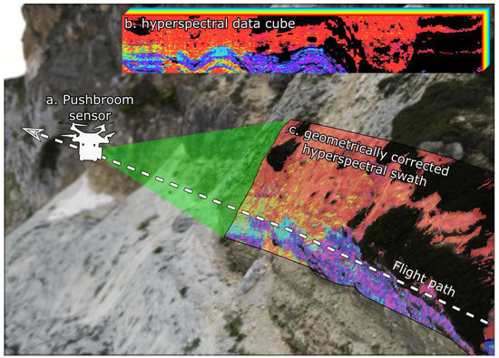
Figure 1.
Data acquisition procedure using a UAV-mounted pushbroom sensor. The sensor is mounted on a UAV, which moves over the target of interest (a) and captures light from within a thin scanline (green) to progressively construct a hyperspectral data cube (b). This data cube must then be geometrically corrected to a spatially accurate hyperspectral swath (c) that can be analysed or interpreted to map, e.g., mineralogy.
For frame-sensors, image matching and computer vision techniques can be used to co-register hyperspectral bands and so correct for geometric distortions [10,16,17]. Pushbroom sensors are more challenging; an inertial processing unit (IMU) and global positioning system (GPS) is needed to accurately quantify the movement of the sensor and remove distortions by back-projection (e.g., [15]). Despite these challenges, several authors have successfully used pushbroom VNIR sensors to collect extremely high-resolution (2–10 cm) data with reasonable levels of spatial accuracy (5–100 cm; [15,18,19,20]). All of these authors corrected distortions resulting from UAV movement using closed-source geometric corrections implemented in the PARGE software [21]. This approach applies a ray-tracing algorithm to locate the centre point of each hyperspectral pixel on a high-resolution digital elevation model (DEM) and then interpolates between these to fill gaps as necessary. Due to uncertainties in measuring sensor position and orientation using an inertial processing unit (IMU), most authors then warp the resulting hyperspectral orthomosaic to fit measured ground control points [21] or a high-resolution photogrammetric RGB orthomosaic [18,20].
Due to their reliance on raster datasets, this correction method performs poorly in topographically complex areas, which cannot be compressed into a 2.5D raster [15]. Areas of geological interest and good exposure, such as cliffs, quarries and mines, often include sub-vertical faces with multiple orientations, so cannot be projected onto a 2D grid (DEM/orthomosaic) without introducing projective distortions that significantly degrade data quality [10,22,23]. To mitigate these issues and facilitate the collection of geological data from potentially important but otherwise inaccessible outcrops, a rapidly increasing number of methods are being developed to fuse remotely sensed hyperspectral data with dense 3D point clouds to create hyperclouds [8,10,17,23,24] that objectively record outcrop geometry and composition.
In this contribution, we present (1) a novel and open-source python workflow for applying robust geometric and radiometric corrections to hyperspectral data, regardless of acquisition and target geometry, and (2) results from a demonstration survey conducted to map the distribution of dolomitic, calcitic and argillaceous carbonate lithologies exposed along cliffs near Passo Giau, Italy (Figure 2). This transect is large enough (>500 × 100 m) to be directly analogous to geological structures resolvable in subsurface seismic data.
2. Location
The study area is located on the south-eastern side of the Gusela del Nuvolau outcrop [25], north of Passo Giau in the central-eastern Italian Dolomites (Figure 2). This 600 m long and 300 m high cliff (Figure 3) exposes remnants of an exhumed Cassian carbonate platform of the Upper Ladinian to Lower Carnian age, including the transition from platform (Cassian Dolomite Formation) to basinal (San Cassiano Formation) facies [26]. The Cassian Dolomite is a greyish-white fine grained dolostone with sucrose texture that, due to the pervasive dolomitisation of the Cassian platform, preserves few original characteristics of the rock (e.g., original textures, fossils or sedimentary structures; [27]). The San Cassiano Formation comprises alternating marls and limestones with oolitic/bioclastic grainstone [26,27]. In general, the geometries of the Cassian platform and the San Cassiano Formation (Figure 3) suggest a north-east (NE) progradation of the slope deposits onto the basinal unit [25,28].
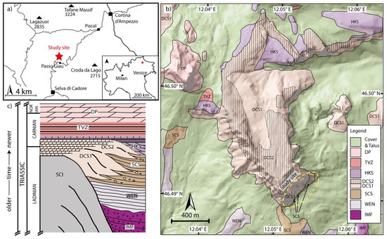
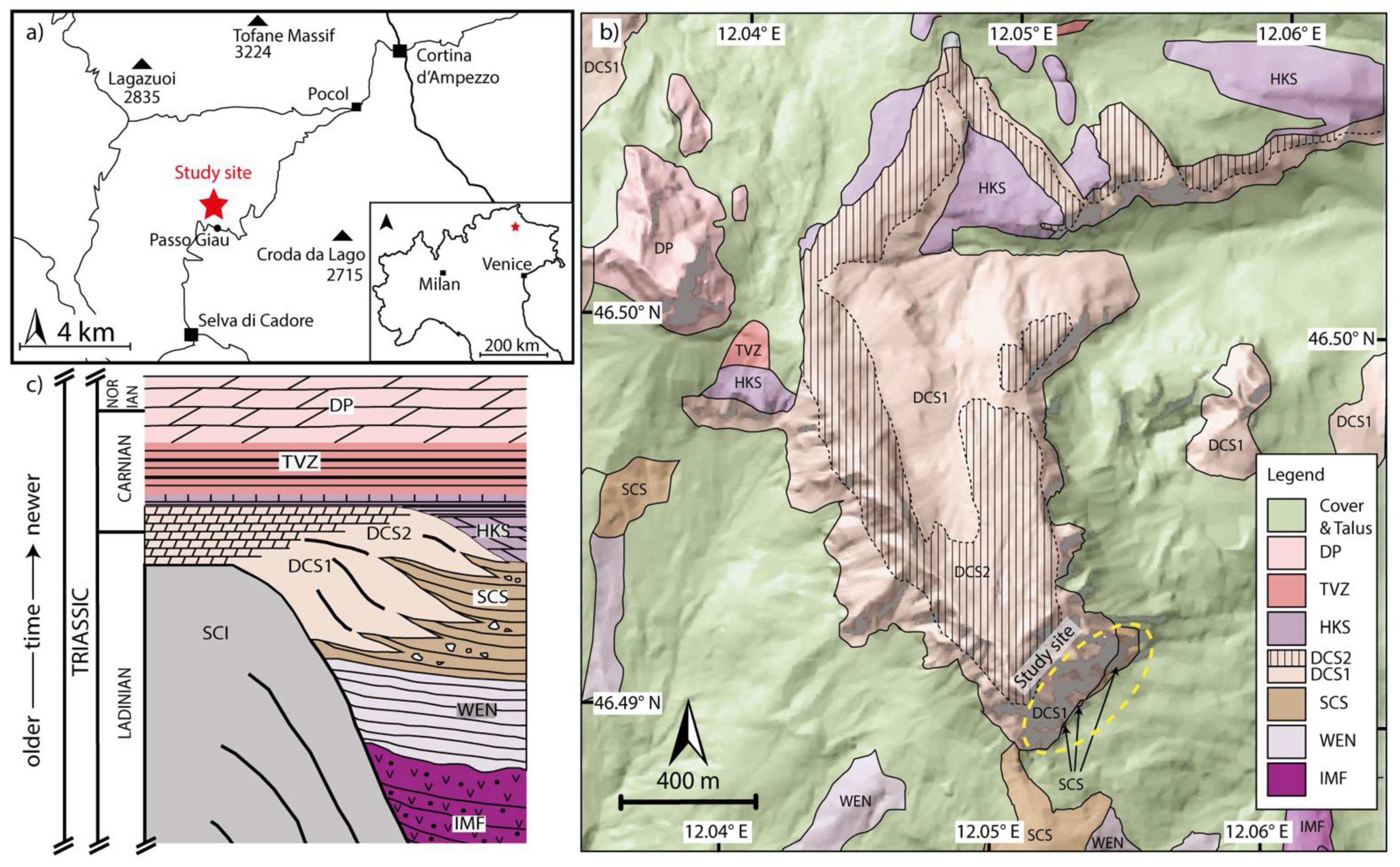
Figure 2.
Location map (a) of the study site and simplified geological map of the surrounding area (b; cf. [27]). The Gusela del Nuvolau outcrop is indicated by the yellow dashed oval. This exposes Middle/Upper Triassic stratigraphy (c) of the central-eastern Italian Dolomites [26]: DP, Dolomia Principale; TVZ, Travenanzes Formation (Fm.); HKS, Heiligkreutz Fm.; DCS, Cassian Dolomite Fm.; SCS, San Cassiano Fm.; WEN, Wengen Fm.; SCI, Sciliar Fm.; IMF, Mt. Fernazza Fm.

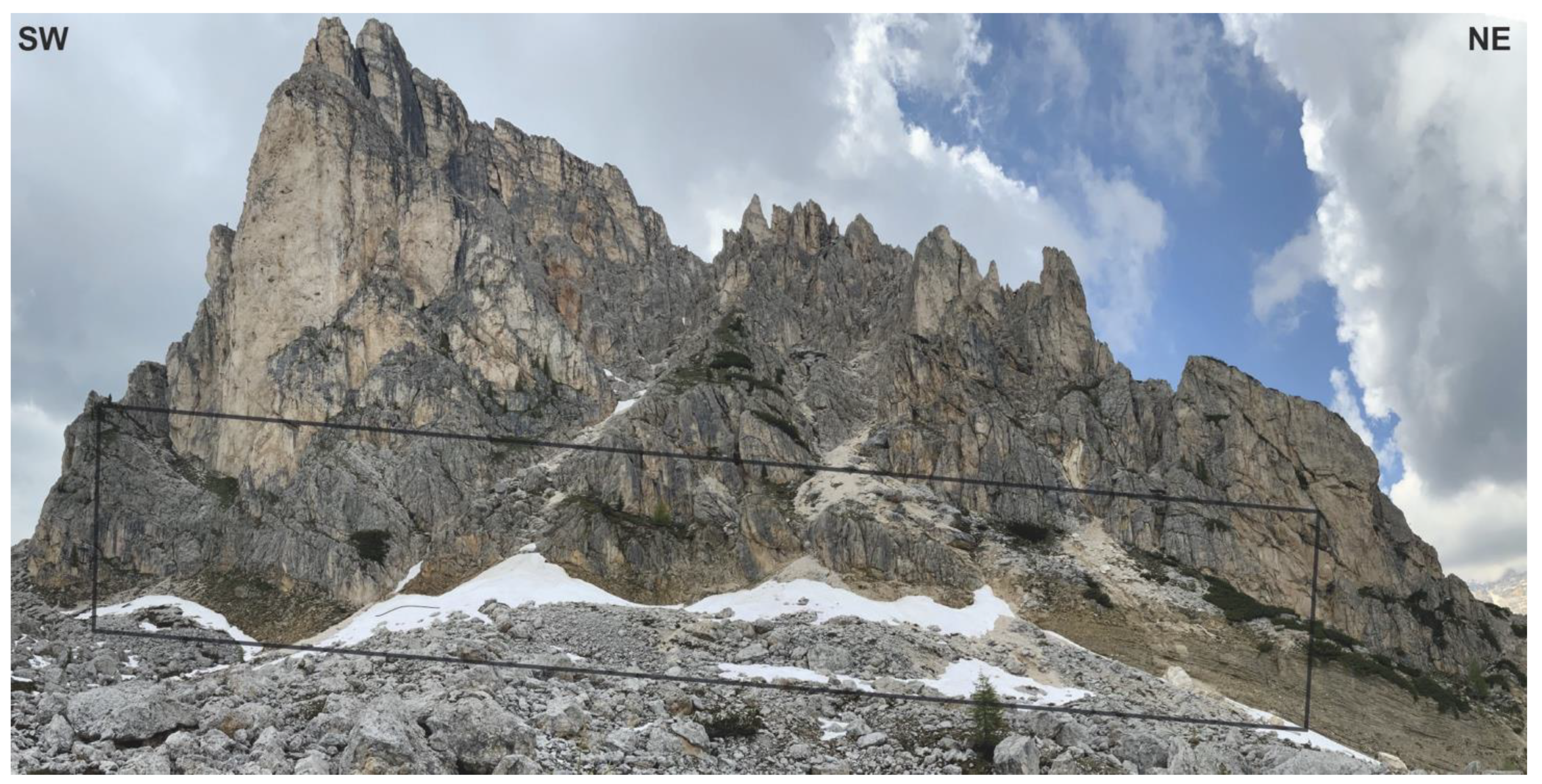
Figure 3.
Photograph of the study area (Gusela del Nuvolau cliff). The carbonate body contains dolomitic and calcitic units, but these cannot be distinguished using the naked eye. Cliff is 250–300 m high and 600 m long. The grey rectangle shows the approximate extent of the hyperspectral survey.
The outcrop is accessible today due to the Alpine orogenic event, during which the Dolomites underwent only mild tectonic deformation [29,30,31]. This allowed preservation of seismic scale depositional geometries of the Middle Triassic platform [25] at Gusela del Nuvolau (Figure 3).
Geological determination of lithofacies partitioning (i.e., quantification of spatial juxtaposition and proportions of geological rock types) are typically obscured by a combination of access limitations and subjective, non-reproducible interpretation by geologists. The primary objectives to deploy the UAV and VNIR-SWIR camera are to provide an accurate and objective method for mapping lithological and mineralogical variations (here calcite, dolomite and clay), which benefits the reconstruction of realistic and accurate models in the subsurface for the energy industry (geothermal, CO2 sequestration and hydrocarbons). The Passo Giau outcrop was selected as a technical test site to demonstrate the method’s potential, test correction procedures and validate the remotely sensed hyperspectral imagery.
3. Methods
3.1. Hyperspectral Data Acquisition
We used a HySpex Mjolnir VS-620 system (Table 1), which allows the concurrent acquisition of hyperspectral data in the VNIR range (400–1000 nm, HySpex Mjolnir V-1240 sensor with 1024 spatial pixels) and the SWIR range (970–2500 nm, HySpex Mjolnir S-620 sensor with 620 spatial pixels). These sensors operate as pushbroom scanners to create a spectral data cube by constant acquisition and movement along the target of interest (Figure 1).

Table 1.
Sensor parameters of the HySpex Mjolnir VS-620 combined hyperspectral imaging and photogrammetry system deployed in the study. Data from the V-1240 were spatially downsampled (binned) to match the S-620 sensor for this study.
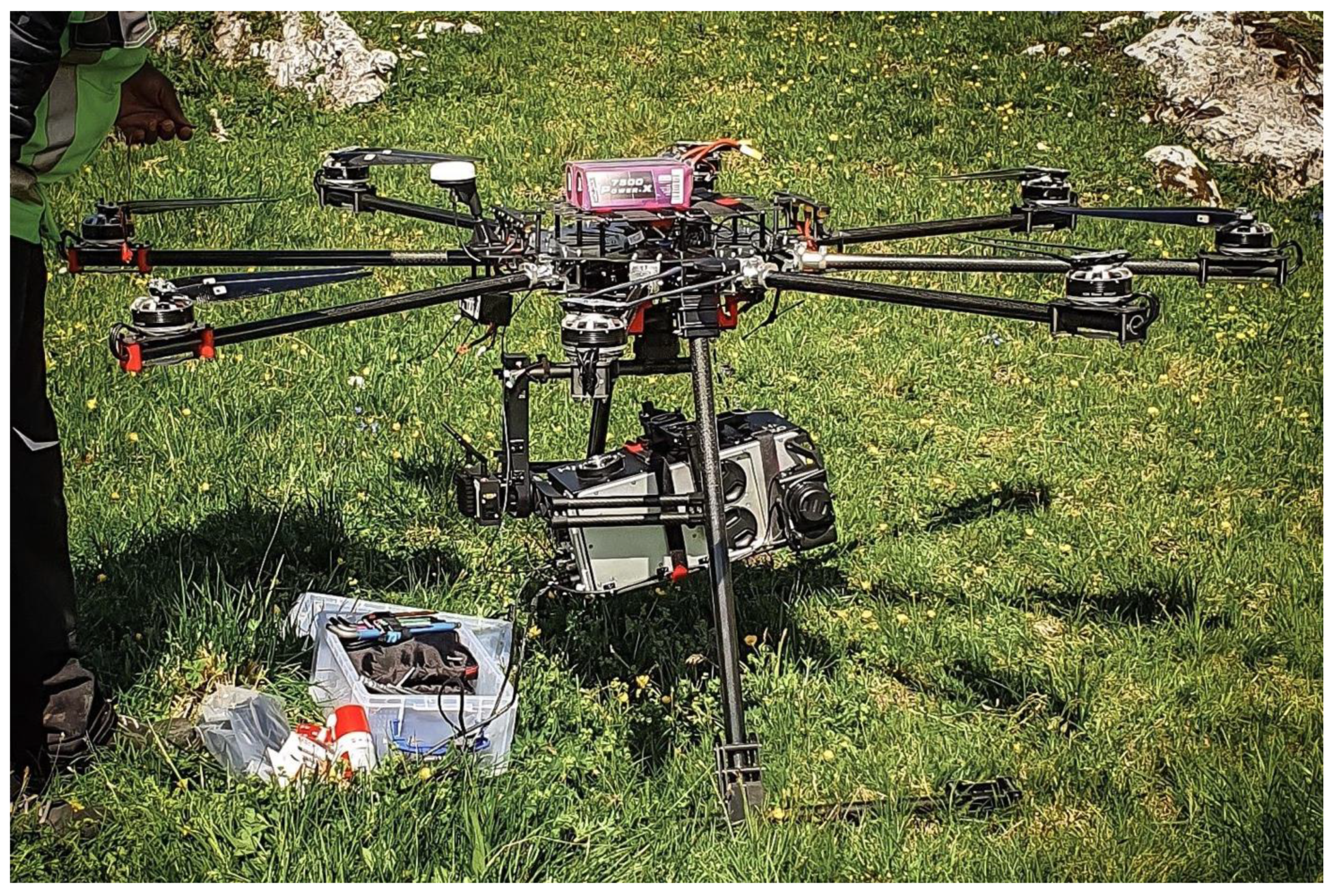
Unlike typical nadir-oriented sensor setups, we mounted the Mjolnir sideways in a Gremsy gStabi H16 XL gimbal so that the camera faced the cliff face and the scan line was sub-vertical. This setup was carried by a custom-built octocopter UAV (Figure 4) which, with the equipped payload of ~8 kg, can achieve flight times of 15–20 min under ideal conditions.
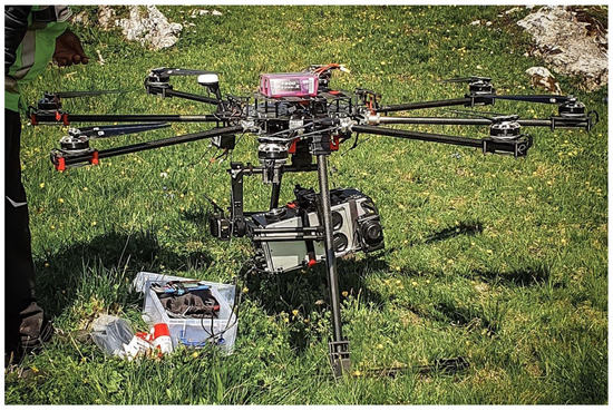
Figure 4.
Image of the UAV and Hyspex Mjolnir-VS mounted sideways in the Gremsy gStabi H16 XL gimbal. Lens caps for the three sensors (VS-1240, S-620 and Sony Alpha) can be seen on the right side of the camera.
In the current study, two swaths of hyperspectral data (hereafter referred to as Swath A and Swath B) were acquired by flying gently descending flight lines (parallel to bedding) at 140 (Swath A) and 90 m (Swath B) distance from the cliff (Figure 5). Due to generally sunny conditions, a frame rate of 50 fps and resulting integration times of 10 (VNIR) and 20 ms (SWIR) was sufficient to ensure adequate image exposure, and a velocity of ~2 m/sec chosen to give approximately square pixels. This configuration resulted in a theoretical ground sampling distance of 8 cm (Flight A) and 5 cm (Flight B) for the SWIR sensor (Table 1).
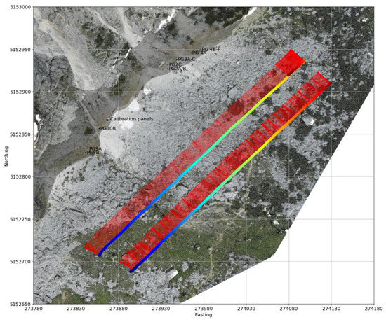
Figure 5.
Post processed flight paths for flight A and B draped over the photogrammetric model. Coloured points show the camera position at each frame (line of hyperspectral data), with blue at the start of each survey and red at the end. The closely spaced red vectors show the camera viewing direction at each of these positions. The transparent grey area shows the map-view extent of the surveyed section of cliff. The location of the Zenith calibration panels (Section 3.5) and ground-truth spectra (Section 3.7) are also overlain for reference.
High winds (~14 m/s) and poor GPS signal presented significant challenges during data acquisition, as pushbroom sensors require flight lines to be conducted in as smooth a fashion as possible. These were (partially) mitigated by orienting the scanner such that it faced the cliff while the UAV was flying forwards, as opposed to orienting the scanner in a forward-facing direction and flying the UAV sideways. This configuration was found to be more stable, because the UAV does not need to constantly manoeuvre to maintain a fixed heading. The gently descending flight lines also helped to stabilise the UAV.
3.2. Photogrammetry
The HySpex Mjolnir camera was also fitted with a co-aligned 24.2 megapixel mirrorless DSLR camera (Sony Alpha 6400) that captured an RGB image every 200 hyperspectral frames, resulting in 205 images with a horizontal overlap of ~80%. These images were supplemented by an additional 144 images captured using a DJI Spark and 132 images from a Parrot Anafi to ensure the entire outcrop was adequately covered, and then processed using Agisoft Metashape (v. 1.6.3 build 10732) to generate a sparse cloud containing 249,329 points using structure from motion (SfM). This sparse cloud was manually filtered to remove outliers and then georeferenced using 14 ground control points surveyed using a PPK GNSS rover (8 points; 3–5 cm accuracy) and Total Station (6 points; ~10 cm accuracy) before re-running the bundle adjustment to mitigate potential photogrammetric distortions. Finally, a dense cloud containing 99,141,154 points was created using the multi-view stereo technique implemented in Agisoft Metashape and exported to CloudCompare [32], where it was subsampled by removing closely spaced points until they had an average spacing of 5 cm, and clipped to the region of interest. Details of the photogrammetric reconstruction can be found in Supplementary Materials 1.
3.3. Geometric Corrections
As with all airborne pushbroom scanners, complex geometric distortions caused by changes in position and orientation of the camera during flight require correction before a usable image can be obtained. These corrections rely on precise position and orientation data recorded by an Applanix APX-20 inertial processing unit (IMU) mounted within the Hyspex Mjolnir camera to model and remove geometric distortions. However, established correction workflows (e.g., [11,15]) rely on 2.5D representations of scene geometry and so cannot correct highly oblique surveys covering e.g., cliffs or open-pit mines. For this reason we have developed and implemented a novel geometric correction procedure within the open-source hylite toolbox (cf. [10]).
First, as was previously described by [15], we processed the APX-20 data using Trimble’s PosPAC software to apply post processed kinematic (PPK) corrections to the GNSS position data and fuse this with accelerometer and orientation measurements from the IMU using the Applanix Inertial Navigation System (INS) fusion toolbox. Data from the onboard GNSS was corrected using a Trimble base station that we set up on site using a Zephyr 2 GNSS Antenna and R5 receiver. The position of our base station was determined using static measurement with an occupation time of 5 h and corrected using Trimble Business Centre and permanent base station data from Bolzano, Bozen, Cercivento, Rovereto, Padova and Venezia.
The cliffs obscured a significant part of the sky during data acquisition, meaning the onboard GNSS receiver only recorded data from 5–12 satellites during the flight, causing highly degraded GNSS solutions (PDOP < 4 for ~30% of the flight time). Because of this, we processed each flight line separately and manually removed the degraded sections. This lowered the overall quality of the processing, especially because it meant only one IMU calibration figure was available for each survey, creating discrepancies between the two flight lines. Each flight was processed twice using the INS fusion algorithm in POSPac; the first solution was used to identify the lever-arm between the GNSS receiver and the IMU, and the second to obtain the final smoothed best estimate (SBET) trajectory.
This trajectory was exported and processed using software provided by Hyspex (Hyspex Nav) to derive camera orientation and position measurements for the pixel-centres of each hyperspectral line (Figure 5). A boresight correction was also applied using HySpex Nav and values determined from ground control points surveyed during a calibration flight conducted by the sensor manufacturer.
We then used hylite [10] to project the photogrammetric point cloud onto the hyperspectral image using the measured position and orientation of the sensor during the acquisition of each line of hyperspectral pixels, and so built a sparse mapping matrix (M) that relates points in the scene to pixels in each swath. M has dimensions such that each row corresponds to a point in the point cloud and each column the (flattened) index of a hyperspectral pixel. Mij thus represents the visibility of point i (with position ui) in pixel j given the camera position vector c and orientation matrix R at the start (n) and end (n + 1) of the hyperspectral frame. Note that unlike conventional frame sensors, pushbroom acquisition modes often image the same point multiple times (due to rotation of the sensor during acquisition), so M represents a many to many mapping between points and pixels.
For pushbroom sensors, a point can be considered to be visible from pixel j if it crossed the sensor scan line during the exposure of this pixel, resulting in a change in sign (sgn) of the dot product between the camera motion vector and relative point position vector (in camera coordinates), satisfying:
This will be true only if the pixel crossed the sensor plane between frames n and n + 1. Points outside the sensor field of view are then culled (based on a perspective projection and focal length f), so that points are only considered visible if they satisfy both Equation (1) and:
where either m = n or m = n + 1 (cf. [33] for an overview of the mathematics behind perspective projection).
Constructing M for large clouds (10–100 million points) and hyperspectral swaths (>1000 s of lines) would require prohibitively expensive computations, as Equations (1) and (2) need to be evaluated for every point and every line of pixels. Our algorithm reduces the number of required computations by dividing each hyperspectral image into 200 pixel wide chunks and, for each chunk, considering only points that cross the sensor plane between its first and last line, and are within the cross-track field of view. This form of frustum culling (a commonly applied technique for rapid 3-D rendering; [33]) significantly reduces the computations required by projecting only a small subset of the total point cloud onto each line of pixels, by assuming the camera position and orientation vary smoothly over time (a requirement for collecting usable data).
To facilitate the identification and removal of occluded points (that map onto the sensor after a perspective projection but were not visible due to a light-blocking object in the foreground), the inverse of the distance between each point-pixel pair were stored as the elements of the mapping matrix M. This allows efficient querying of point-pixel depths (by computing the argmax of M along its columns) and the construction of a depth buffer [33] that can be used to identify and remove elements in M that result from occluded points.
Different normalisations or filtering can then be applied to M to derive a normalised mapping matrix, denoted Mf, which can be multiplied by a vector of pixel spectra (Ps) or point attributes (Va) to derive back-projected per-point point spectra (Vs) or a projected image of point attributes (Pa):
The normalisation method will determine how many to many relationships between points and pixels will be handled. If Mf is calculated by normalising M such that its columns sum to one, then the spectra in all of the pixels that a point is visible from will be averaged (weighted by their proximity to the sensor). Alternatively, the number of points contained in each pixel (which is proportional to the on-ground pixel size, or footprint) can be calculated by summing the columns of M and used to derive a filtered Mf that maps the spectra from the closest (smallest footprint) pixel directly to each point (with no averaging), so that maximum spatial resolution is retained.
Code for constructing M and performing these filtering operations to rapidly transfer data between a SfM-MVS point clouds and pushbroom hyperspectral imagery has been implemented in python as part of the open-source hylite package and is available at https://github.com/samthiele/hylite (accessed on 16 December 2021).
3.4. Boresight Optimisation
Despite the accuracy of the Applanix IMU under optimal conditions, a combination of GPS error, IMU orientation uncertainty, and the boresight between the IMU and each hyperspectral sensor, resulted in a relatively large offset (1–2 m/10–20 pixels) between projected hyperspectral pixels and their actual location on the point cloud (identified using RGB colours from the SfM-MVS). These errors were not ameliorated by applying a standard boresight calibration using values estimated using SfM during the earlier calibration flight (cf. [15]), probably because they result from rotations of the local coordinate system induced by poor GPS signal during the survey and IMU calibration figure (cf. Section 3.3), rather than the physical sensor boresight. This unacceptably large error was reduced by developing a novel boresight optimisation algorithm that finds the boresight values which result in the highest correlation between projected RGB colours and equivalent colours in the SfM-MVS point cloud.
First, we assume that the combined IMU alignment errors can be approximated by a single rigid body rotation between the IMU and the SfM-MVS point cloud coordinate systems. Position errors most likely also result in a lever-arm offset, but this constant offset will have less effect on projected pixel location than orientation error (which increases proportionally to the sensor–target distance).
An optimal boresight adjustment was then found to correct this rotation (IMU misalignment) for each flight line, by repeatedly projecting the red, green and blue bands of each of the VNIR images onto a sub-sampled point cloud and maximising the correlation with point colours derived from the SfM-MVS model. This optimisation was achieved using the iterative least-squares algorithm implemented in SciPy (scipy.optimise.minimize; [34]).
Following this procedure, we were able to co-register the two hyperspectral swaths to within ~1 pixel of each other, and ~2 pixels of the SfM-MVS point cloud (based on a visual assessment of the projected point colours; Figure 6). A quantitative assessment of the reprojection error was not possible, as surveyed ground control points could not be placed on the cliffs. The projection-mapping matrix calculated using the boresight values was then saved for each flight for subsequent use during radiometric correction (Section 3.5) and fusion of the swaths (Section 3.6).
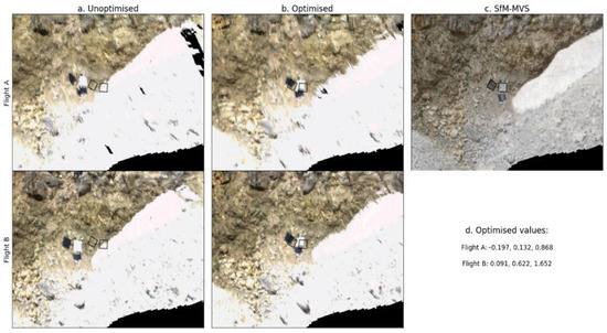
Figure 6.
Geometrically corrected true-colour hyperspectral datasets before (a) and after (b) boresight optimisation for each flight. Outlines of the 1 m2 grey and black calibration panels as mapped on the SfM-MVS point cloud (c) are overlain for reference. While there is significant room for improvement, coregistration error dropped from ~2.5 m before optimisation to ~0.2 m afterwards. Interestingly the optimal boresight values (roll, pitch, yaw in degrees) are substantially different between the two flights (d), even though these were conducted within an hour of each other. This suggests that they represent ‘virtual’ boresight values that correct for a misalignment between the global coordinate system and the IMU coordinate system caused by poor GPS signal during IMU calibration, rather than the real sensor boresight.
3.5. Radiometric Corrections
The hyperspectral data for each flight were preprocessed using dedicated software provided by HySpex (HyspexRad) to convert raw digital numbers into radiance and correct for smile and keystone distortions. Calibration spectra from two Zenith calibration panels (R = 5% and 50%) placed at the base of the cliff in each scene (cf. Figure 5) were then extracted by back-projection onto a subset point cloud containing only the panels. Additionally, indirect illumination was quantified by averaging pixels of a shaded Spectralon R90 panel (R = 90%) that was placed in front of the camera following each survey (after the UAV had landed).
Following the method of [35], these spectra were used to characterise the downwelling sunlight, skylight and path radiance in each scene. The measured radiance (r) of each panel with known reflectance spectra R can be described by the approximately Lambertian reflection of a mixture of diffuse skylight and sunlight [35]:
where I and S are the incident sunlight (direct illumination) and skylight (indirect illumination) spectra, respectively; a is the fraction of visible sky from the panel, θ is the angle between the panel normal and downwelling sunlight and P is the path radiance. We find the three unknowns in this equation (S, I and P) by solving the following linear system:
where A, B and C correspond to each of the three panels used (5%, 55% and the (shaded) 90% panel, respectively). The panels’ sky view factor (a) and incidence angle (θ) were calculated using the SfM-MVS model, as described in the following paragraph. Note that the inclusion of a fully shaded panel (such that for this panel I is known to be 0) ensures proper characterisation of approximately omnidirectional skylight (cf. [35]).
These three illumination spectra (Figure 7c,d) allowed us to model and correct for the influence of atmospheric and topographic effects. As described in detail by [35], incident and viewing angles for each pixel were calculated by projecting the 3-D point cloud onto each hyperspectral image (cf. Equation (4)) and computing an Oren-Nayar [36] bidirectional reflectance distribution function (BRDF) that simulates the fraction α of sunlight reflected towards the camera from each pixel. Sky view factors (a) were calculated for each point using the PCV plugin [37] in CloudCompare, and projected from the point cloud onto each pixel in the hyperspectral image. This allowed per-pixel reflectance (R) to be estimated from measured radiance (r) using the following equation [35]:
where the numerator represents the at-target reflected radiance, and the denominator the combined direct and indirect illumination across the scene.
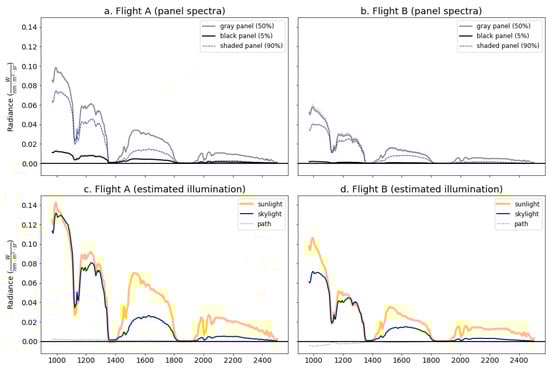
Figure 7.
Measured calibration panel spectra (a,b) for each flight and derived illumination source spectra (c,d). These spectra were used to model and correct for illumination effects (atmospheric and topographic) separately in each flight. Note that the path radiance is essentially negligible, as expected due to the short sensor–target distance, but that skylight accounts for 25% to 50% of the total illumination during both flights.
3.6. Fusion and Minimum Wavelength Mapping
Due to the differing survey distances (cf. Figure 5), the swath from Flight A covered a wider extent than Flight B, but at lower resolution. Thus, after applying the radiometric and geometric corrections described in Section 3.4 and Section 3.5, they were fused to derive a combined dataset with optimal spatial coverage and resolution. The spectra from each swath were projected onto two separate hyperclouds using a filtered mapping matrix Mf that back-projects the smallest-footprint pixel onto each point in the SfM-MVS cloud (cf. Section 3.3). Then, the per-point spectra from each swath were averaged using a weighting factor proportional to each pixel’s ground-sampling distance, such that the two surveys were averaged to combine their extent and (slightly) reduce spectral noise, but without significantly compromising spatial resolution.
Finally, a hull-correction from 2100–2500 nm was applied to this merged hypercloud to emphasise absorption features related to clay and mica minerals in the shales (~2200 nm), calcite (~2345 nm) and dolomite (~2325 nm) and create the false-colour composite presented in Section 4. Minimum wavelength mapping of absorption feature position and depth (cf. [38,39,40,41]) was then performed using the multi-gaussian absorption feature-fitting algorithm implemented in hylite. This was used to simultaneously fit the three main mineralogical absorption features (AlOH, FeOH and CO3) expected in the range 2150–2360 nm, and thus allow discrimination between the different minerals at Passo Giau.
3.7. Collection of Validation Spectra
Point spectra measurements were conducted using a portable spectrometer to provide ground truth data for validating the remotely sensed spectra. Ten sampling sites were selected based on an on-site evaluation of the geology and stratigraphy, access limitations and to ensure spatial coverage of the extent of the outcrop. Ten measurements were collected at each of these sites, covering the range of dominant facies or micro-facies (as interpreted by the geologist), using a FieldSpec spectrometer equipped with a contact probe that allowed measurements of the reflectance spectra from areas of ~1 cm2. These sampling sites were then marked using spray-on chalk such that they could be easily identified in the photogrammetric model of the area. Of these sites, 5 overlapped with the extent of the UAV survey and could be identified in the photogrammetric point cloud, allowing equivalent spectra to be sampled from within ±1 m of the spray-on chalk markers and within the relevant microfacies (as identified based on field observations and interpretation of the photogrammetric model).
4. Results
The geometric correction and boresight optimisation routine described in Section 3.3 and Section 3.4 allowed successful correction and georeferencing of the raw hyperspectral swaths (Figure 8), despite collection under adverse conditions (significant wind and poor GPS signal) to produce a geometrically and radiometrically corrected hypercloud. Jupyter notebooks showing the application of these methods are available in the Supplementary Material.
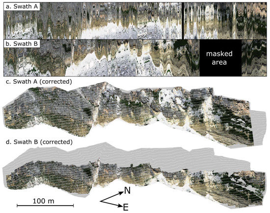
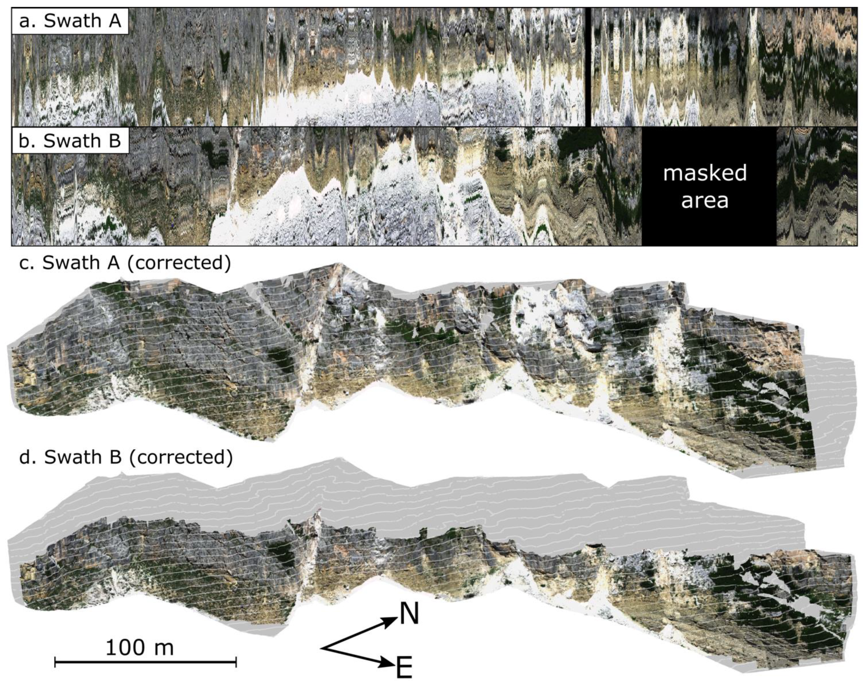
Figure 8.
True colour uncorrected (a,b) and geometrically corrected (c,d) visualisations of each hyperspectral swaths. Although spatial accuracy is limited to ~2 pixels (Figure 5), the extensive geometric distortions in the original images have been almost entirely corrected. The 3-m spaced horizontal contours are overlain in white for reference. Areas in the original images occluded by the leg of the drone have been masked to prevent projection onto the point-cloud. Note that the duplication of pixels in the raw hyperspectral swaths means that this did not leave gaps in the geometrically corrected results.
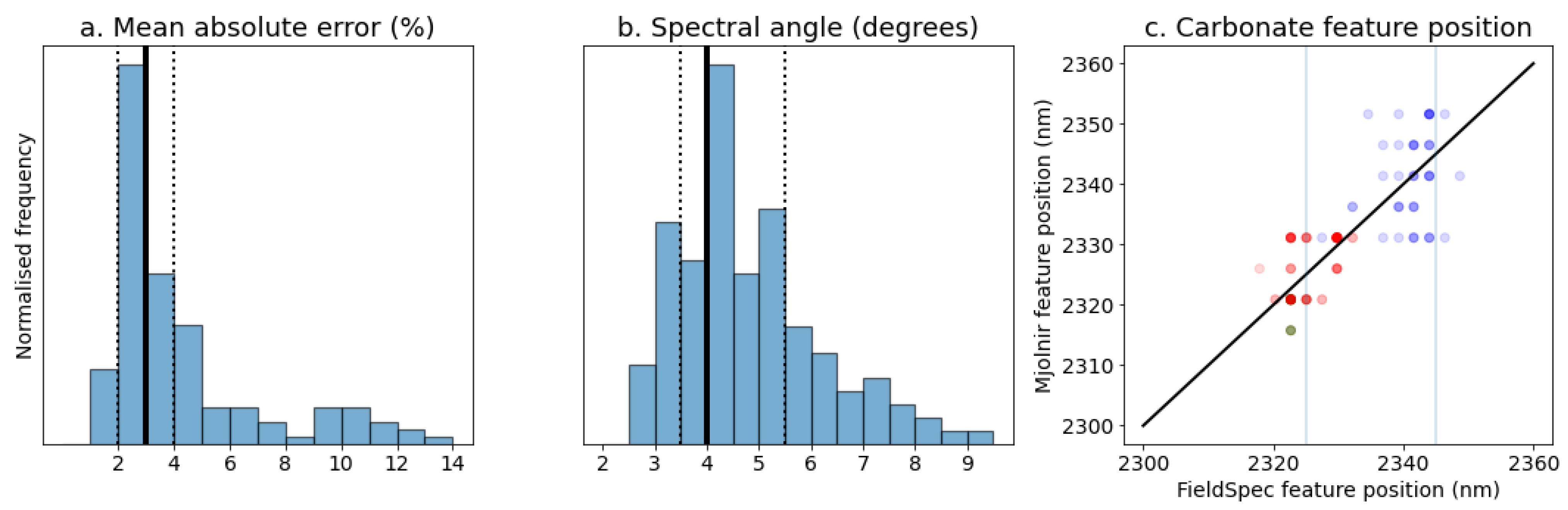
The resulting point-spectra closely match those measured in situ using the FieldSpec (Figure 9). The Mjolnir and FieldSpec spectra were compared by calculating the mean average error (MAE; sensitive to spectra shape and magnitude) and spectral angle (SA; sensitive to spectra shape only) between the Mjolnir and closest FieldSpec spectra at each of the reference sites (Figure 10). These suggest that the majority of the remotely sensed Mjolnir spectra are accurate to 2–4% (MAE) and 3.5–5.5° (SA). Considering the significant challenges associated with remotely sensing accurate reflectance spectra, we consider these errors to be acceptable.
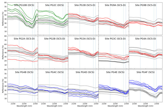
Figure 9.
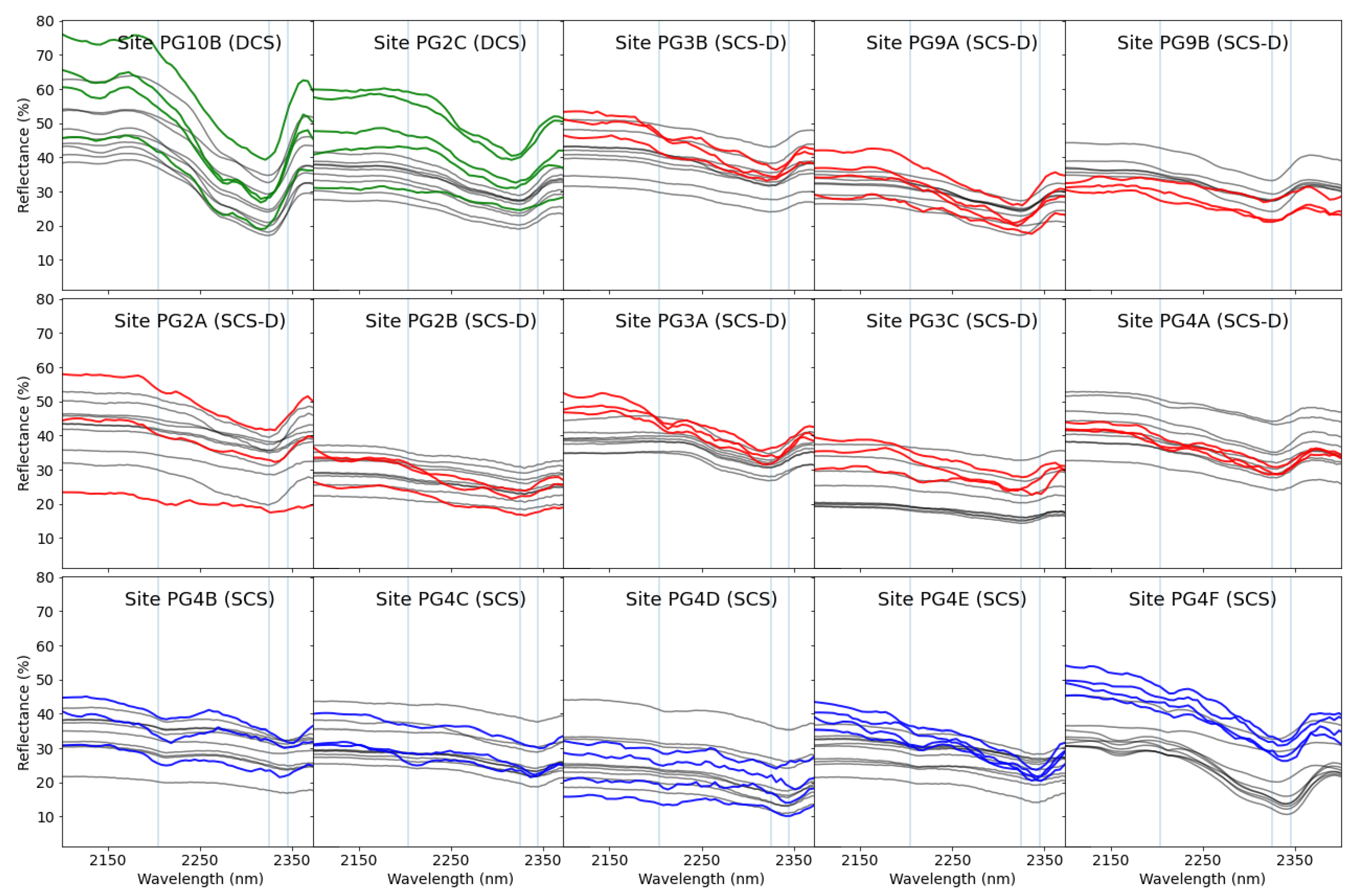
Comparison of corrected HySpex Mjolnir spectra and ground truth FieldSpec measurements (plotted in grey) from the Cassian Dolomite Formation (DCS; green), dolomitised San Cassiano Formation (SCS-D; red), and calcitic San Cassiano Formation (SCS; blue). The location of these validation sites is plotted in Figure 4 and Figure 11. Note that these measurements were used to check the spectral accuracy of the UAV data, not to validate a classification or lithological map of the outcrop; so lithological unit labels provided above are for reference only. Blue vertical lines show the expected positions of the AlOH, dolomitic CO3 and calcitic CO3 absorption features mapped in Figure 11 and Figure 12.
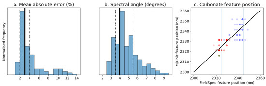
Figure 10.
Quantitative error metrics showing the mean absolute error (a) and spectral angle (b) between the HySpex Mjolnir and corresponding FieldSpec measurements. Vertical black line shows the median error and vertical dotted lines the 25th and 75th percentiles. A comparison of the carbonate absorption position measured using the different instruments is shown in (c), and shows that the ~20 nm shift in absorption feature position between calcite and dolomite can be resolved in both datasets, allowing calcitic lithotypes to be distinguished from dolomitic ones (point colour corresponds to the different stratigraphic units; cf. Figure 9). Vertical blue lines show the expected position for dolomite (2325 nm) and calcite (2345 nm).
Figure 9 and Figure 10 also show that the Mjolnir and FieldSpec spectra consistently identify variations in the position and depth of the AlOH and CO3 absorption features (at ~2200 and 2320–2345 nm, respectively). These subtle differences were be used to map the dominant mineralogy across the outcrop, and so discriminate the fine-grained dolostone of the Cassian Dolomite Formation (DCS; Figure 9) from the interbedded micritic limestone and marls of the San Cassiano Formation (SCS; Figure 9), and their dolomite equivalents (SCS-D; Figure 9). SCS and SCS-D both show an AlOH feature indicating the presence of clay minerals, while the position of the CO3 feature distinguishes calcitic SCS (2345 nm) from dolomitic SCS-D and DCS (2325 nm).
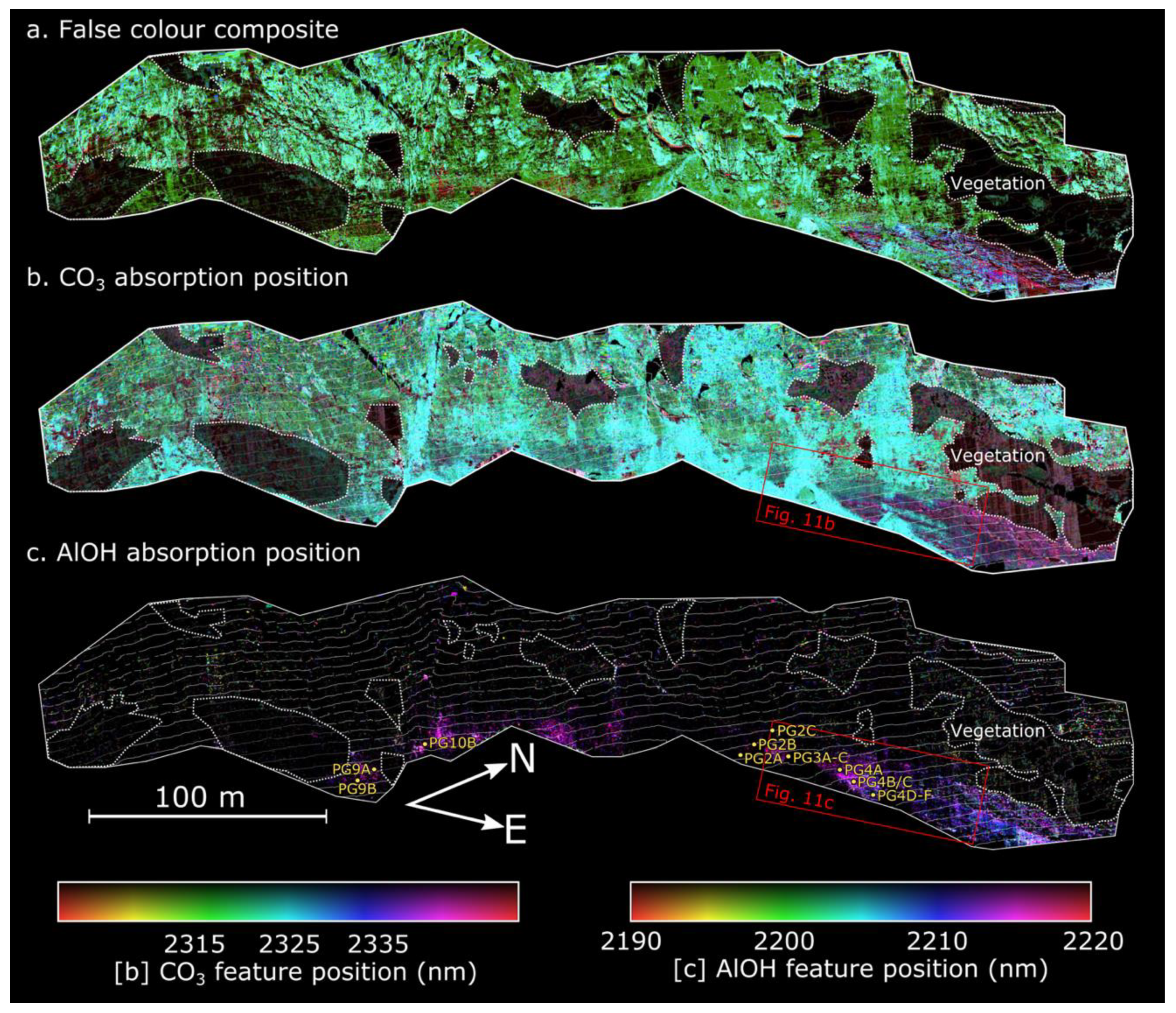
The false colour visualisation (Figure 11a) created using the absorption depth at 2200, 2320 and 2340 nm highlights these differences, clearly distinguishing dolostone (green) from limestone (blue), as well as shale-rich argillites (purple to red). Similarly, the minimum wavelength map shows variations in the position of the CaCO3 absorption feature from 2320 nm (dolomite) to 2340 nm (calcite), providing a visualisation of the calcite to dolomite ratio (Figure 11b). The calcitic limestone (2340–2345 nm) can be clearly distinguished from overlying dolomites (2315–2325 nm), and correlates with argillites (San Cassiano Fm) identified based on their distinct texture (fine laminations) in the photogrammetric model and abundant clay or mica minerals identified by mapping the depth of the 2200 nm AlOH absorption feature (Figure 11c).
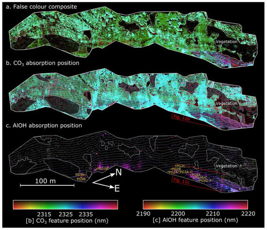
Figure 11.
False-colour visualisation of the merged and radiometrically corrected hypercloud (a) and minimum wavelength maps showing the distribution of calcitic (blue) and dolomitic (green) carbonates (b) and clay/mica minerals (purple; c). The location of the validation spectra shown in Figure 9 are overlain on (c) in yellow for reference.
Interestingly, some of this limestone has been dolomitised to a distance of ~2–5 m along its top contact (Figure 12), an observation that would likely have been missed if the unit was mapped using only traditional methods. A geoscience interpretation of these results is beyond the scope of this current work, but we present some preliminary interpretations in the following section (Section 5). The false colour visualisations and minimum wavelength map results can downloaded from https://tinyurl.com/nuvolau (accessed on 16 December 2021).
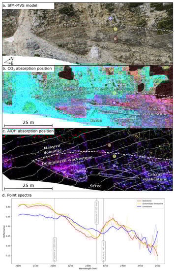
Figure 12.
Close-up of the dolostone-limestone contact (dashed white line) showing the stratigraphically crosscutting transition zone containing dolomitised limestone in the true-colour SfM-MVS model (a), and carbonate (b) and AlOH (c) absorption feature minimum wavelength maps. Note that the image has been rotated to make bedding sub-horizontal; thin white lines show 3-m spaced horizontal contour lines. Example reflectance spectra (d) sampled from the coloured circles in (a–c) are plotted for reference. These spectra (dotted lines) were smoothed (solid lines) using a Savitzky–Golay filter with a window size of 7 and polynomial order of 2, to reduce noise and highlight the clear shift in absorption position from 2345 nm (calcite) to 2325 nm (dolomite). Refer to Figure 11 for the colour scales used in (b,c).

5. Discussion
Our results highlight the significant potential of UAV-compatible SWIR hyperspectral cameras for creating detailed, accurate and objective geological maps in inaccessible terrain. As shown in Figure 9, Figure 10 and Figure 11, the remotely mapped SWIR spectra are accurate and can distinguish the lithologies and mineral alteration (dolomitisation) at a scale and resolution that would be difficult with ground-based sensors or field mapping. While care must be taken to fully understand potential weathering effects [42,43], these data significantly supplement the high resolution geometric and textural information captured using conventional digital outcrop mapping techniques, and specifically contribute to provide a detailed map of mineralogy across the slope to basin transition at Gusela de Nuvolau. Potential applications of this approach are far broader than mapping carbonate mineralogy in reservoir analogues, and include, e.g., mapping clays, mica and chlorite associated with hydrothermal alteration around mineral deposits or volcanic edifices for minerals exploration or geohazard assessment.
A few geological studies have employed UAV hyperspectral SWIR cameras (e.g., [14]), but we suggest that significant potential for the development and innovative application of both methods remains. We hope that our novel processing approach helps to realise this potential, by (1) facilitating accurate corrections in areas of steep terrain (e.g., cliffs or open pit mines) and (2) retaining true 3-D information by avoiding the need to project data into a 2-D orthomosaic. The former is significant as areas of exceptional geological exposure are rarely flat, while the latter avoids gridding and reprojection artefacts associated with DEM-based workflows (cf. [23]), as real pixel footprints are retained in M, and also results in point cloud data suited for digital outcrop analysis (e.g., LIME, CloudCompare, VRGS; [32,44,45]) or 3-D modelling.
To demonstrate this, we used VRGS [45] to perform a preliminary interpretation of the hyperspectral mineral mapping results and associated SfM-MVS point cloud (Figure 13). This synthesises the mineral-mapping results with high resolution textural information captured by the SfM-MVS model and regional knowledge to help better constrain the stratigraphic nature of the slope to basin relationship (e.g., slope breccia downlapping on basin wedge or interfingering), as well as the spatial reach of the dolomitisation fluids from coarse slope sediments to basinal, thin bedded, fine-grained limestone intervals alternating with shales and marls (Figure 13). Part of the dolomitising fluids are interpreted here to have circulated throughout faults and connected fractures (Figure 13), laterally invading porous and permeable rock volumes. Adjacent non-porous and impermeable basinal facies acted as a barrier to dolomitising fluids, preserving the associated rock type from dolomitisation. Dolomitisation processes are complex and multiphase in the Dolomites region, and are not in the scope of this study. Instead, this contribution proves the reliability of the developed technology and workflow, opening opportunities to acquire similar, unbiased and accurate, geometrical and mineralogical information along vertical outcrops, with major implications for the evaluation of subsurface analogues for geothermal, CO2 sequestration and conventional hydrocarbon exploration and production.
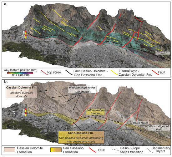
Figure 13.
Digital outcrop interpretation of the Gusela del Nuvolau cliff based on the SfM-MVS model and hyperspectral survey data. The minimum wavelength map (cf. Figure 11 and Figure 12) has been overlain in (a) as a reference. This clearly shows the gradational and stratigraphically crosscutting dolomitisation of the otherwise calcitic San Cassiano Formation (b), and that the Cassian Dolomite Formation has been completely dolomitised.
However, as with any remote sensing technology employing UAVs, data acquisition is particularly sensitive to field conditions (e.g., weather and GPS signals). The high winds and poor GPS reception we experienced during data acquisition emphasise the need for robust processing solutions that can accurately correct data from an erratically moving platform. Our novel geometric correction and boresight optimisation routines are a step in this direction, and allowed us to extract accurate data in spite of the adverse conditions, but there remains significant room for improvement. Tools for planning automated UAV surveys that use non-nadir camera angles (due to topographic complexity) are also lacking, especially if high-resolution topographic information is unavailable. Small-scale commercial solutions are beginning to emerge from the engineering inspection industry (Skydio; www.skydio.com, accessed on 16 December 2021), but these currently cannot be employed for high-payload drones.
Finally, we suggest that good quality analysis and control (QAQC) procedures that can be applied while in the field to ensure sufficient data quality are needed. Some progress has been made on applying geometric corrections in real-time [46], but more needs to be done to make these solutions available, robust and field-ready. Appropriate field QAQC is essential for many geological studies, as field locations are often inaccessible and visiting multiple times is impractical or prohibitively expensive. Real-time processing capabilities also allow adaptation of survey plans and acquisition parameters when areas of interest are identified, and potentially validated or ground-truthed while onsite. By implementing our method in the open-source hylite toolbox we hope to facilitate advances in these directions to realise the potential of rapidly developing UAV hyperspectral imaging technologies.
6. Conclusions
We provide an open-source toolbox for the accurate correction of non-nadir pushbroom hyperspectral data. Our robust algorithm allows the processing of VNIR and SWIR data acquired obliquely and targeting outcrops with complex geometries, such as cliffs or mines. In a first step, this algorithm was developed for the Hyspex NEO Mjolnir, but we expect users to be able to use our tools to process data from any pushbroom sensor, provided a detailed photogrammetric outcrop model is also available. The procedure is included in the open-source hylite package (https://github.com/samthiele/hylite, accessed on 16 December 2021), and the authors welcome further contributions. We demonstrated the potential of this toolbox using data collected in conditions representative of operational acquisitions. Despite non-optimal weather and GPS reception, distortions and related artefacts could be successfully corrected to derive a coherent and spectrally accurate dataset. This contribution opens the door to new UAV hyperspectral acquisition types and supports the development of UAV-based imaging in Earth sciences.
Supplementary Materials
The following are available online at https://www.mdpi.com/article/10.3390/rs14010005/s1, S1: Agisoft Metashape processing report, N1: IMU Visualisation notebook, N2a: Flight A geometric corrections notebook, N2b: Flight B geometric corrections notebook, N3a: Flight A illumination corrections notebook, N3b: Fight B illumination corrections notebook, N4: Data fusion notebook, N5: Minimum wavelength mapping notebook
Author Contributions
Conceptualisation by R.G., J.K., S.T.T., E.D. and S.L.; methodology, S.T.T., Z.B. and S.L.; software, S.T.T., Z.B. and Y.M.; validation, S.T.T., N.M., A.B., E.D. and J.K.; writing—original draft preparation, S.T.T., S.L., Z.B., A.B. and N.M.; writing—review and editing, S.T.T., S.L., A.B., R.G., E.D. and J.K.; project administration, R.G. and J.K.; funding acquisition, R.G. and J.K. All authors have read and agreed to the published version of the manuscript.
Funding
The authors would like to acknowledge funding from TotalEnergies, The European Social Fund (ESF) and the State of Saxony.
Data Availability Statement
Data presented in this study are available at https://doi.org/10.6084/m9.figshare.17126321.v1, accessed on 16 December 2021.
Conflicts of Interest
The authors declare no conflict of interest.
References
- Bemis, S.; Micklethwaite, S.; Turner, D.; James, M.R.; Akciz, S.; Thiele, S.T.; Bangash, H.A. Ground-based and UAV-Based photogrammetry: A multi-scale, high-resolution mapping tool for structural geology and paleoseismology. J. Struct. Geol. 2014, 69, 163–178. [Google Scholar] [CrossRef]
- Dering, G.M.; Micklethwaite, S.; Thiele, S.T.; Vollgger, S.A.; Cruden, A.R. Review of drones, photogrammetry and emerging sensor technology for the study of dykes: Best practises and future potential. J. Volcanol. Geotherm. Res. 2019, 373, 148–166. [Google Scholar] [CrossRef]
- Janiszewski, M.; Uotinen, L.; Merkel, J.; Leveinen, J.; Rinne, M. Virtual Reality Learning Environments for Rock Engineering, Geology and Mining Education. In Proceedings of the 54th U.S. Rock Mechanics/Geomechanics Symposium (ARMA-2020-1101), Golden, CO, USA, 28 June–1 July 2020. [Google Scholar]
- Nesbit, P.; Durkin, P.R.; Hugenholtz, C.H.; Hubbard, S.; Kucharczyk, M. 3-D stratigraphic mapping using a digital outcrop model derived from UAV images and structure-from-motion photogrammetry. Geosphere 2018, 14, 2469–2486. [Google Scholar] [CrossRef] [Green Version]
- Marques, A.; Horota, R.K.; de Souza, E.M.; Kupssinskü, L.; Rossa, P.; Aires, A.S.; Bachi, L.; Veronez, M.R.; Gonzaga, L.; Cazarin, C.L. Virtual and digital outcrops in the petroleum industry: A systematic review. Earth-Sci. Rev. 2020, 208, 103260. [Google Scholar] [CrossRef]
- Laukamp, C.; Rodger, A.; LeGras, M.; Lampinen, H.; Lau, I.; Pejcic, B.; Stromberg, J.; Francis, N.; Ramanaidou, E. Mineral Physicochemistry Underlying Feature-Based Extraction of Mineral Abundance and Composition from Shortwave, Mid and Thermal Infrared Reflectance Spectra. Minerals 2021, 11, 347. [Google Scholar] [CrossRef]
- Kurz, T.H.; Buckley, S.J.; Howell, J.A. Close-range hyperspectral imaging for geological field studies: Workflow and methods. Int. J. Remote Sens. 2013, 34, 1798–1822. [Google Scholar] [CrossRef]
- Kurz, T.H.; Buckley, S.J.; Howell, J.A.; Schneider, D. Integration of panoramic hyperspectral imaging with terrestrial lidar data. Photogramm. Rec. 2011, 26, 212–228. [Google Scholar] [CrossRef]
- Lorenz, S.; Salehi, S.; Kirsch, M.; Zimmermann, R.; Unger, G.; Vest Sørensen, E.; Gloaguen, R. Radiometric Correction and 3D Integration of Long-Range Ground-Based Hyperspectral Imagery for Mineral Exploration of Vertical Outcrops. Remote Sens. 2018, 10, 176. [Google Scholar] [CrossRef] [Green Version]
- Thiele, S.T.; Lorenz, S.; Kirsch, M.; Acosta, I.C.C.; Tusa, L.; Herrmann, E.; Möckel, R.; Gloaguen, R. Multi-scale, multi-sensor data integration for automated 3-D geological mapping. Ore Geol. Rev. 2021, 136, 104252. [Google Scholar] [CrossRef]
- Aasen, H.; Honkavaara, E.; Lucieer, A.; Zarco-Tejada, P.J. Quantitative Remote Sensing at Ultra-High Resolution with UAV Spectroscopy: A Review of Sensor Technology, Measurement Procedures, and Data Correction Workflows. Remote Sens. 2018, 10, 1091. [Google Scholar] [CrossRef] [Green Version]
- Kim, J.; Chi, J.; Masjedi, A.; Flatt, J.E.; Crawford, M.M.; Habib, A.F.; Lee, J.; Kim, H. High-resolution hyperspectral imagery from pushbroom scanners on unmanned aerial systems. Geosci. Data J. 2021. [Google Scholar] [CrossRef]
- Goldstein, N.; Wiggins, R.; Woodman, P.; Saleh, M.; Nakanishi, K.; Fox, M.E.; Tannian, B.E.; Ziph-Schatzberg, L.; Soletski, P. Compact visible to extended-SWIR hyperspectral sensor for unmanned aircraft systems (UAS). In Proceedings of the Algorithms and Technologies for Multispectral, Hyperspectral, and Ultraspectral Imagery XXIV, Bellingham, WA, USA, 17–19 April 2018; Volume 10644, p. 106441G. [Google Scholar]
- Barton, I.F.; Gabriel, M.J.; Lyons-Baral, J.; Barton, M.D.; Duplessis, L.; Roberts, C. Extending geometallurgy to the mine scale with hyperspectral imaging: A pilot study using drone- and ground-based scanning. Min. Met. Explor. 2021, 38, 799–818. [Google Scholar] [CrossRef]
- Arroyo-Mora, J.; Kalacska, M.; Inamdar, D.; Soffer, R.; Lucanus, O.; Gorman, J.; Naprstek, T.; Schaaf, E.; Ifimov, G.; Elmer, K.; et al. Implementation of a UAV–Hyperspectral Pushbroom Imager for Ecological Monitoring. Drones 2019, 3, 12. [Google Scholar] [CrossRef] [Green Version]
- Booysen, R.; Jackisch, R.; Lorenz, S.; Zimmermann, R.; Kirsch, M.; Nex, P.A.M.; Gloaguen, R. Detection of REEs with lightweight UAV-based hyperspectral imaging. Sci. Rep. 2020, 10, 17450. [Google Scholar] [CrossRef] [PubMed]
- Kirsch, M.; Lorenz, S.; Zimmermann, R.; Tusa, L.; Möckel, R.; Hödl, P.; Booysen, R.; Khodadadzadeh, M.; Gloaguen, R. Integration of Terrestrial and Drone-Borne Hyperspectral and Photogrammetric Sensing Methods for Exploration Mapping and Mining Monitoring. Remote Sens. 2018, 10, 1366. [Google Scholar] [CrossRef] [Green Version]
- JuanManuel, J.R.; Padua, L.; Hruska, J.; Feito, F.R.; Sousa, J.J. An Efficient Method for Generating UAV-Based Hyperspectral Mosaics Using Push-Broom Sensors. IEEE J. Sel. Top. Appl. Earth Obs. Remote Sens. 2021, 14, 6515–6531. [Google Scholar] [CrossRef]
- Turner, D.; Lucieer, A.; McCabe, M.; Parkes, S.; Clarke, I. Pushbroom Hyperspectral Imaging from an Unmanned Aircraft System (UAS)—Geometric Processingworkflow and Accu-racy Assessment. ISPRS Int. Arch. Photogramm. Remote Sens. Spat. Inf. Sci. 2017, XLII-2/W6, 379–384. [Google Scholar] [CrossRef] [Green Version]
- Angel, Y.; Turner, D.; Parkes, S.; Malbeteau, Y.; Lucieer, A.; McCabe, M.F. Automated Georectification and Mosaicking of UAV-Based Hyperspectral Imagery from Push-Broom Sensors. Remote Sens. 2020, 12, 34. [Google Scholar] [CrossRef] [Green Version]
- Schlaepfer, D.; Schaepman, M.E.; Itten, K.I. PARGE: Parametric geocoding based on GCP-calibrated auxiliary data. SPIE’s Int. Symp. Opt. Sci. Eng. Instrum. 1998, 3438, 334–344. [Google Scholar] [CrossRef]
- Ghamisi, P.; Shahi, K.R.; Duan, P.; Rasti, B.; Lorenz, S.; Booysen, R.; Thiele, S.; Contreras, I.C.; Kirsch, M.; Gloaguen, R. The Potential of Machine Learning for a More Responsible Sourcing of Critical Raw Materials. IEEE J. Sel. Top. Appl. Earth Obs. Remote Sens. 2021, 14, 8971–8988. [Google Scholar] [CrossRef]
- Inamdar, D.; Kalacska, M.; Arroyo-Mora, J.P.; Leblanc, G. The Directly-Georeferenced Hyperspectral Point Cloud: Preserving the Integrity of Hyperspectral Imaging Data. Front. Remote Sens. 2021, 2, 9. [Google Scholar] [CrossRef]
- Buckley, S.; Kurz, T.H.; Howell, J.A.; Schneider, D. Terrestrial lidar and hyperspectral data fusion products for geological outcrop analysis. Comput. Geosci. 2013, 54, 249–258. [Google Scholar] [CrossRef]
- Bosellini, A. Progradation geometries of carbonate platforms: Examples from the Triassic of the Dolomites, northern Italy. Sedimentology 1984, 31, 1–24. [Google Scholar] [CrossRef]
- Neri, C.; Gianolla, P.; Furlanis, S.; Caputo, R.; Bosellini, A. Note Illustrative Della Carta Geologica d’Italia. In Foglio Cortina D’ampezzo 029; ISPRA: Rome, Italy, 2007. [Google Scholar]
- Inama, R.; Menegoni, N.; Perotti, C. Syndepositional fractures and architecture of the lastoni di formin carbonate platform: Insights from virtual outcrop models and field studies. Mar. Pet. Geol. 2020, 121, 104606. [Google Scholar] [CrossRef]
- Blendinger, W.; Blendinger, E. Windward-leeward effects on Triassic carbonate bank margin facies of the Dolomites, northern Italy. Sediment. Geol. 1989, 64, 143–166. [Google Scholar] [CrossRef]
- Bosellini, A.; Neri, C. The Sella Platform. Dolomieu Conference on Carbonate Platforms and Dolomitization; Guidebook Excursion B; KARO-Druck: Ortisei, Italy, 1991. [Google Scholar]
- Cadrobbi, L.; Nobile, G.; Lutterotti, G. Studio Di Supporto Alla Stesura Del Piano Regolatore Generale Del Comune Di Canazei, Studio Associato Di Geologia Applicata; Canazei, Italy, 1995; Volume 1955-1. [Google Scholar]
- Mollema, P.N.; Antonellini, M. Development of strike-slip faults in the dolomites of the Sella Group, Northern Italy. J. Struct. Geol. 1999, 21, 273–292. [Google Scholar] [CrossRef]
- Girardeau-Montaut, D. CloudCompare. 2020. Available online: https://cloudcompare.org/ (accessed on 16 December 2021).
- Akenine-Moller, T.; Haines, E.; Hoffman, N. Real-Time Rendering; AK Peters/crc Press: Natick, MA, USA, 2019; ISBN 1-315-36545-6. [Google Scholar]
- Virtanen, P.; Gommers, R.; Oliphant, T.E.; Haberland, M.; Reddy, T.; Cournapeau, D.; Burovski, E.; Peterson, P.; Weckesser, W.; Bright, J.; et al. SciPy 1.0: Fundamental algorithms for scientific computing in Python. Nat. Methods 2020, 17, 261–272. [Google Scholar] [CrossRef] [PubMed] [Green Version]
- Thiele, S.T.; Lorenz, S.; Kirsch, M.; Gloaguen, R. A Novel and Open-Source Illumination Correction for Hyperspectral Digital Outcrop Models. IEEE Trans. Geosci. Remote Sens. 2021, 14, 1–12. [Google Scholar] [CrossRef]
- Oren, M.; Nayar, S.K. Seeing beyond Lambert’s law. In Proceedings of the Computer Vision—ECCV ’94; Springer: Berlin/Heidelberg, Germany, 1994; pp. 269–280. [Google Scholar]
- Berthaume, M.A.; Winchester, J.; Kupczik, K. Ambient occlusion and PCV (portion de ciel visible): A new dental topographic metric and proxy of morphological wear resistance. PLoS ONE 2019, 14, e0215436. [Google Scholar] [CrossRef]
- Huguenin, R.L.; Jones, J.L. Intelligent information extraction from reflectance spectra: Absorption band positions. J. Geophys. Res. Space Phys. 1986, 91, 9585–9598. [Google Scholar] [CrossRef]
- Van der Meer, F. Analysis of spectral absorption features in hyperspectral imagery. Int. J. Appl. Earth Obs. Geoinf. 2004, 5, 55–68. [Google Scholar] [CrossRef]
- Van Ruitenbeek, F.; Bakker, W.H.; van der Werff, H.; Zegers, T.E.; Oosthoek, J.H.; Omer, Z.A.; Marsh, S.; van der Meer, F.D. Mapping the wavelength position of deepest absorption features to explore mineral diversity in hyperspectral images. Planet. Space Sci. 2014, 101, 108–117. [Google Scholar] [CrossRef]
- Sunshine, J.; Pieters, C.M.; Pratt, S.F. Deconvolution of mineral absorption bands: An improved approach. J. Geophys. Res. Space Phys. 1990, 95, 6955–6966. [Google Scholar] [CrossRef] [Green Version]
- Beckert, J.; Vandeginste, V.; McKean, T.J.; Alroichdi, A.; John, C.M. Ground-based hyperspectral imaging as a tool to identify different carbonate phases in natural cliffs. Int. J. Remote Sens. 2018, 39, 4088–4114. [Google Scholar] [CrossRef] [Green Version]
- Kurz, T.H.; San Miguel, G.; Dubucq, D.; Kenter, J.; Miegebielle, V.; Buckley, S.J. Quantitative Mapping of Dolomitization Using Close-Range Hyperspectral Imaging: Kimmeridgian Carbonate Ramp (Alacón, NE Spain). Geosphere 2022, in press. [Google Scholar]
- Buckley, S.J.; Ringdal, K.; Naumann, N.; Dolva, B.; Kurz, T.H.; Howell, J.A.; Dewez, T.J. LIME: Software for 3-D visualization, interpretation, and communication of virtual geoscience models. Geosphere 2019, 15, 222–235. [Google Scholar] [CrossRef]
- Hodgetts, D.; Gawthorpe, R.L.; Wilson, P.; Rarity, F. Integrating Digital and Traditional Field Techniques Using Virtual Reality Geological Studio (VRGS). In Proceedings of the 69th EAGE Conference and Exhibition Incorporating SPE EUROPEC 2007; EAGE Publications BV: Utrecht, The Netherlands, 2007; p. cp-27-00300. [Google Scholar]
- Koirala, P.; Løke, T.; Baarstad, I.; Fridman, A.; Hernandez, J. Real-time hyperspectral image processing for UAV applications, using HySpex Mjolnir-1024. In Proceedings of the Algorithms and Technologies for Multispectral, Hyperspectral, and Ultraspectral Imagery XXIII; SPIE: Bellingham, WA, USA; Washington, DC, USA, 2017; Volume 10198, p. 1019807. [Google Scholar]


Publisher’s Note: MDPI stays neutral with regard to jurisdictional claims in published maps and institutional affiliations. |
© 2021 by the authors. Licensee MDPI, Basel, Switzerland. This article is an open access article distributed under the terms and conditions of the Creative Commons Attribution (CC BY) license (https://creativecommons.org/licenses/by/4.0/).