LPIN: A Lightweight Progressive Inpainting Network for Improving the Robustness of Remote Sensing Images Scene Classification

Abstract

At present, the classification accuracy of high-resolution Remote Sensing Image Scene Classification (RSISC) has reached a quite high level on standard datasets. However, when coming to practical application, the intrinsic noise of satellite sensors and the disturbance of atmospheric environment often degrade real Remote Sensing (RS) images. It introduces defects to them, which affects the performance and reduces the robustness of RSISC methods. Moreover, due to the restriction of memory and power consumption, the methods also need a small number of parameters and fast computing speed to be implemented on small portable systems such as unmanned aerial vehicles. In this paper, a Lightweight Progressive Inpainting Network (LPIN) and a novel combined approach of LPIN and the existing RSISC methods are proposed to improve the robustness of RSISC tasks and satisfy the requirement of methods on portable systems. The defects in real RS images are inpainted by LPIN to provide a purified input for classification. With the combined approach, the classification accuracy on RS images with defects can be improved to the original level of those without defects. The LPIN is designed on the consideration of lightweight model. Measures are adopted to ensure a high gradient transmission efficiency while reducing the number of network parameters. Multiple loss functions are used to get reasonable and realistic inpainting results. Extensive tests of image inpainting of LPIN and classification tests with the combined approach on NWPU-RESISC45, UC Merced Land-Use and AID datasets are carried out which indicate that the LPIN achieves a state-of-the-art inpainting quality with less parameters and a faster inpainting speed. Furthermore, the combined approach keeps the comparable classification accuracy level on RS images with defects as that without defects, which will improve the robustness of high-resolution RSISC tasks.

1. Introduction

Remote Sensing (RS) images are widely used in earth science, agriculture, military reconnaissance, disaster rescue and many other fields. To fully understand and utilize the rich information of the earth surface contained in RS images, the task of RS images scene classification (RSISC) has become a research hotspot. Most existing RSISC methods [1] can be roughly divided into two categories according to their approaches to feature designing and extracting. One is the traditional machine learning-based methods with hand-crafted features, such as models based on Bag of Visual Words (BoVW) [2], Randomized Spatial Partition (RSP) [3], Hierarchical Coding Vector (HCV) [4] and Fisher vectors (FVs) [5]. As deep learning technology has been proved to have excellent performance in computer vision and pattern recognition [6,7], the classification methods based on Convolutional Neural Network (CNN) [8,9,10,11,12,13,14,15,16,17,18,19] have been widely investigated for they can learn and extract image features automatically. Hu et al. [9] and Du et al. [10] used a pretrained CNN to extract image features. Yin et al. [11] defined three types of fusion-based models for RSISC and gave typical fusion methods. Li et al. [12] proposed a hybrid architecture of a pre-trained model combined with an unsupervised encoding method. Wang et al. [13] adopted an attention module and constructed an end-to-end network. Li et al. [14], Jiang et al. [15], and Zhang et al. [16] used Capsule Network (CapsNet) in their model which can preserve the spatial information of RS images. To date, the RSISC tasks have achieved a quite high-level accuracy on standard datasets. For instance, the overall accuracy (OA) is 94.87% [16] on the NWPU-RESISC45 dataset [20] and 96.05% [16] on the Aerial Image Dataset (AID) [21], both with a training ratio of only 20%. Moreover, the RS image classifications using the red-green-blue band of EuroSAT dataset [22] achieves an accuracy of 99.17% via deep transfer learning [23].

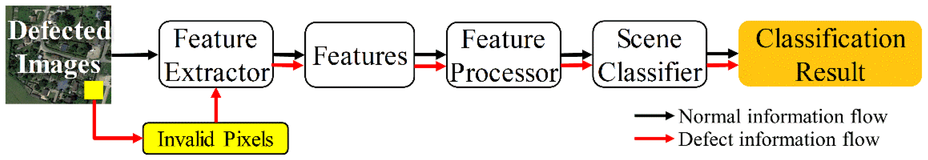
1.1. The Dilemma of Existing RSISC Methods

As reviewed above, the existing RSISC methods have performed well on standard RS image datasets, but cannot achieve a similar accuracy on real RS images, which usually have defects due to satellite sensors failures and atmospheric environment disturbances. Three typical defects exist in real RS images: (1) Periodic stripes. On 31 May 2003, the off problem of Landsat-7 Enhanced Thematic Mapper Plus (ETM+) Scan-Line Corrector (SLC) resulted in a stripe shape pixel loss in the images acquired since then. (2) Random noises. The electromagnetic interference between the satellite optical sensors and the load devices often generates random noises and leads to dead pixels in RS images. (3) Thick clouds. Thirty-five percent of the earth surface is covered by clouds [24], which makes it difficult to obtain pure RS images without clouds. In summary, the defects in real RS images will inevitably introduce invalid pixel interferences to RSISC tasks.

Experimental results in this paper show that the classification accuracy of a well performed model on the standard dataset may decrease by 68.05% at most when dealing with the defected RS images. The existing RSISC tasks take the defected RS images as the input and the invalid pixels directly participate in feature extracting as shown in Figure 1. These invalid pixels induce a defect information flow during the feature processing and might lead to the misclassification of scene classifier and the decrease of classification accuracy. Therefore, we believe that the existing RSISC tasks face a dilemma of accurate classification on real RS images with defects. The task of improving the robustness of RSISC methods and maintaining their classification accuracy on real RS images with defects is crucial for practical application of RSISC and is also the research emphasis of this paper.

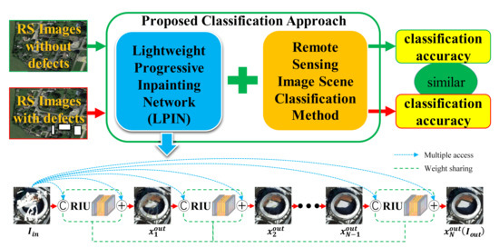
1.2. The Approach to Overcoming this Dilemma

A variety of methods have been proposed to reduce the interference of defects in the defected images. For example, Li et al. [25] replaced several layers in the model with discrete wavelet transform. Duan et al. [26] designed image features that are insensitive to defects. Chen et al. [27] proposed a method to learn the statistical characteristics of defects and used image filters to separate the defects. Chen et al. [28] also adopted a spectral-spatial preprocessing algorithm to improve the performance of the hyperspectral RS image classification. However, these methods are mainly designed for enhancing the anti-defect capability of their models instead of eliminating defects. Various modules are adopted in the models to decrease interference of the defects, which leads to an increase in the complexity and training time of the model.

In addition, to apply the inpainting network on small portable systems such as RS unmanned aerial vehicles (UAV) for practical application of RSISC tasks, the models must be lightweight due to the restriction of memory and power consumption, which we believe is also one of the current challenges dealing with the defect RS images and needs to be paid extra attention to.

At present, few studies on improving the robustness of RSISC from the perspective of purifying the input images and lightweight design have been reported. Thus, to solve the dilemma fundamentally, we propose a Lightweight Progressive Inpainting Network (LPIN) based on the lightweight design, and a novel approach to purifying the front-end input RS images as shown in Figure 2 instead of improving the anti-defect ability of the back-end classification methods.

Different from the commonly used image preprocessing methods, such as image filtering, the proposed LPIN focuses on the image reconstruction to generate a completely new RS image and cut off the defect information flow introduced by invalid pixels. The LPIN has a light model weight and a fast computing speed which ensures it is suitable for the practical application of RSISC tasks. Then, it is combined with existing RSISC methods to extract purified features and improve the classification accuracy and the robustness of RSISC tasks. Besides, the proposed approach also has a wide applicability and can be adopted to multiple back-end classification methods.

1.3. Related Works of Image Inpainting

The image inpainting technology is used to reconstruct the images with undesired regions, it involves a branch of image reconstructions and has been widely applied in computer vision [29], such as human face repairing, mosaic removal, watermark removal, cultural heritage image restoration and so on. For RS images inpainting, patch matching based on probability and statistics theories are the most widely used methods. They aim at searching and matching suitable patches in valid regions and copy them to the corresponding defect regions [30,31,32,33]. Zheng et al. [34] inpainted the hyperspectral RS images with Nonlocal Second-order Regularization (NSR) and used semi-patch to accelerate nearest neighbor searching. Zhuang et al. [35] proposed a Fast Hyperspectral Denoising (FastHyDe) model and a Fast Hyperspectral Inpainting (FastHyIn) model to deal with defects in hyperspectral RS images. Li et al. [36] used Patch Matching-based Multitemporal Group Sparse Representation (PM-MTGSR) with auxiliary images to inpaint the defect region caused by thick cloud occlusion and sensor faults. Lin et al. [37] used the temporal correlation of RS images to create patch clusters in the temporal and spatial layers, and searched and matched the missing information from the clusters to inpaint the cloud-contaminated images. These methods can inpaint the defects in RS images, but if there are no suitable patches in the valid regions or the defect regions to be inpainted have complex structures, the inpainting often gives unsatisfactory results.

Compared with the patch-based methods, the deep learning-based methods can achieve much better inpainting performance because they can learn from the image content and style automatically and comprehend the image globally. Pathak et al. [38] proposed a Context Encoder (CE) model, which proved the feasibility of CNN for image inpainting. Since then, various architectures and modules have been developed to generate more reasonable and realistic inpainting results. However, in the practical use of RSISC tasks on small portable systems, the inpainting network needs to have less parameters and a lightweight structure due to the restriction of memory and power consumption. However, in the field of image inpainting, researchers mainly focused on designing new modules or architectures and neglected the lightweight of networks.

For example, to maintain consistency of local texture and global content, Iizuka et al. proposed a Generative Adversarial Networks (GAN) [39] based model Global and Local Consistent Image Completion (GLCIC) [40] with a local discriminator and a global discriminator. To extract distant contextual information for the image missing part of an image, Yu et al. [41] released a coarse-to-fine inpainting network DeepFill based on Wasserstein GAN (WGAN) [42]. To extract valid multi scale features, Liu et al. [43] carried out a Partial Convolution (PCONV) layer with U-net [44] architecture. To avoid treating all image pixels as legal ones, Yu et al. [45] proposed a method called DeepFill v2 using a gated convolution to replace the vanilla convolution in the network. To generate structural information of different scales for a reasonable structured image, Li et al. [46] adopted two Progressive Reconstructions of a Visual Structure (PRVS) layer in the encoder-decoder network. To avoid excessive smoothness and blurring, Nazeri et al. [47] proposed the EdgeConnect method which first generates an edge map and then learns the prior knowledge from the edge map to obtain the result. To ensure the semantic relevance and context continuity of the edges of missing part, Liu et al. [48] adopted a Coherent Semantic Attention (CSA) layer to the generator of GAN. To infer the defects region progressively, Li et al. [49] used a Recurrent Feature Reasoning (RFR) module. To generate a variety of reasonable inpainting results, Zhao et al. [50] came up with Unsupervised Cross-Space Translation GAN(UCTGAN). In terms of RS image inpainting, Dong et al. [51] proposed a model based on Deep Convolutional GAN (DCGAN) [52]. To inpaint the RS Sea Surface Temperature (SST) images. Zhang et al. [53] used a space-time-spectral framework based on CNN to inpaint periodic stripes and thick clouds in satellite RS images. Wong et al. [54] came up with an adaptive spectral feature extraction method to inpaint hyperspectral images using spectral features and spatial information.

As reviewed above, these researchers did not pay attention to the inpainting task from the perspective of lightweight design and also did not care about the complexity of the models and the inpainting time consumption.

Table 1. The size of pretrained model weight of different inpainting models.

Inpainting Method	GLCIC [40]	DeepFill [41]	PCONV [43]	DeepFill v2 [45]	PRVS [46]	Edge-Connect [47]	RFR [49]	PGN [55]	Proposed LPIN
Pretrained Model Weight (MB)	23.2	130.8	412.5	176.4	666.7	38.1	374.8	3132.8	1.2

shows the pretrained weight size of several inpainting models mentioned above. We can see that their models often have large weights which are not suitable for portable systems and thus cannot be directly applied to the practical application of RS image inpainting.

Unlike the existing inpainting methods, the proposed network LPIN is based on the innovative consideration of lightweight inpainting for RS images. As far as we know, this is the first time that an inpainting network is designed from a lightweight perspective. To fully realize a lightweight design, we first disassemble the complex inpainting task into simple tasks by applying a multi-stage progressive architecture, which makes the inpainting task easier for each substage. Afterwards, we adopt the weight sharing strategy among different stages to reduce the network parameters. Then, we enhance the information transmission by adopting a residual architecture and a multi-access of the input images to provide feature reuse in forward propagation and reduce gradients diffusion in backward propagation. Finally, we improve the inpainting performance by restricting the network with multiple loss functions. All these measures work together to give a lightweight but effective inpainting network. According to our experiments, the proposed lightweight network can achieve a state-of-the-art inpainting performance without complex modules and architectures.

1.4. Contribution

Our contributions are summarized as follows:

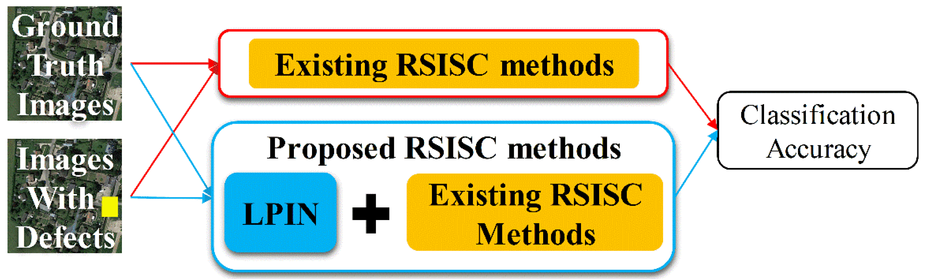
• A novel approach to improving the robustness of RSISC tasks is proposed, which is the combination of an image inpainting network and an existing RSISC method. Unlike the commonly used image preprocessing methods, the approach focuses on the image reconstruction to generate a completely new RS image. To our knowledge, this is the first attempt that image inpainting method has been applied to improve the robustness of RSISC tasks.
• An inpainting network LPIN is proposed on the novel consideration of lightweight design. Compared with the existing inpainting models, the LPIN has a model weight of only 1.2 MB, which is much smaller than other models and is more suitable for practical application of RSISC tasks when implementing it on small portable systems. In spite of the small model weight, the LPIN still remains a state-of-the-art inpainting performance due to the progressive inpainting strategy, residual architecture and the multi-access of input images, which deepen the LPIN and guarantee a high feature and gradient transmission efficiency.
• The proposed approach has a wide applicability and can be adopted to various RSISC methods to improve their classification accuracies on images with defects. The results of extensive experiments show that the proposed approach on RS images with defects generally achieves a classification accuracy of more than 94% (maximum 99.9%) of that on the images without defects. This proves that it can greatly improve the robustness of RSISC tasks.

2. Materials and Methods

A well performed image inpainting network is essential for improving the robustness of RSISC tasks. Combined with this inpainting network, existing classification methods can achieve satisfactory results on the images with defects. In this section, we focus on architecture of the inpainting network LPIN. A basic Residual Inpainting Unit (RIU) is first proposed, with which the defect parts of RS images are preliminarily inpainted. The progressive architecture of the LPIN is then discussed in detail, from which the final inpainting results are obtained. Finally, various loss functions are used to generate more reasonable and realistic results. The overall inpainting architecture of the proposed approach is shown in Figure 3.

2.1. Basic Residual Inpainting Unit

The proposed RIU is a basic inpainting block with a residual architecture, as shown in Figure 3a. It inpaints the defects and generates a preliminarily result. The input $x^{in}$ of RIU concatenates with the real image with defected image $I_{in}$ to form a 6-channel feature, which is processed through two convolution layers, four Residual Blocks (ResBlocks) and one convolution layer in succession to produce a residual result $x^{res}$. The final output of RIU $x^{out}$ is obtained by a pixel-wise addition of $x^{res}$ and $I_{in}$. All convolution layers in RIU have 3 × 3 filters.

The features in ResBlocks $x$ are updated as follows:

$$x=\sigma \left(Res\left(x\right)+x\right)$$

(1)

where $Res$ is the ResBlock and $\sigma$ is the activation function ReLU. The ResBlock creates shortcuts in RIU, i.e., extra path, which makes the transmission of image features and gradients more efficient. The shortcuts ensure a deep network and prevent it from underfitting and gradient diffusion. Firstly, only a part of the feature information is extracted by convolution layer during the forward propagation, and thus, the deeper the network is, the more the information loss is, which causes underfitting. The shortcuts solve this problem by passing the features of the former block to the subsequent blocks to provide an extra information for them. Besides, gradients in deep network are prone to diffuse during backward propagation. With the shortcuts, the later blocks transfer not only the gradients to the former block, but also the gradients before derivation. This means the gradients of each block are amplified, thus reducing the probability of gradient diffusion.

Furthermore, small filter convolution is adopted in the RIU to reduce the number of network parameters. Although large filter convolution gives a better perception of image features, it widens the network and increases its parameter number, which will restrict the depth of a network. According to reference [56], a combination of several small filter convolution layers is equal to that of a large filter convolution layer in the performance of perceiving images while reducing the parameter number. Besides, as the defect regions in RS image are scattered and each single region is relatively small, a small filter convolution is more flexible.

2.2. Progressive Networks

A progressive multi-stage framework is adopted to form a deep network and achieve a better performance. As shown in Figure 3b, the proposed LPIN is composed of several RIUs, which take the output of one as the input for another. With the LPIN, the inpainting task is split into several simpler sub-tasks, and each sub-task inpaints part of the defects progressively. The i-th RIU takes the output of (i − 1)-th RIU $x_{i-1}^{out}$ as its input $x_i^{in}$, which means that the prior knowledge of the (i − 1)-th RIU is transmitted to the i-th RIU. This makes it easier to inpaint the defects for the subsequent RIUs. Multiple RIUs directly increase the depth of LPIN while not increasing its width due to the small filter convolution layer used.

Multiple accesses of the input image $I_{in}$ as shown in the blue dashed lines in Figure 3b are adopted to each RIU to guarantee enough depth for the LPIN. The input of the i-th RIU is a concatenation of $I_{in}$ and its own input $x_i^{in}$, which takes full advantage of the valid feature in $I_{in}$. Meanwhile, the output of the i-th RIU is a pixel-wise addition of $I_{in}$ and its own residual output $x_i^{res}$, with which the RIU forms a larger scale of residual structure. With these multiple accesses, LPIN establishes extra paths. The features and gradients can be directly passed to the top/bottom layers during forward and backward propagation, and the LPIN can become deeper by adding more RIUs while reducing the risk of gradient diffusion.

Weight sharing is another way to guarantee enough depth for the LPIN as the green dashed boxes in Figure 3b show. The more RIUs are adopted in LPIN, the longer the gradient propagation chain is, which might lead to over-fitting and gradient explosion or diffusion during backward propagation. In our network, each RIU shares their weights in a way that parameters are updated after each iteration in the training process and then synchronized to each RIU at the same time. The weight sharing strategy ensures a deeper but lightweight model while reducing the number of parameters, and preventing over-fitting and gradient explosion or diffusion.

2.3. Loss Functions

In addition to the progressive architecture of the LPIN, multiple loss functions are also adopted to achieve reasonable and realistic results as shown in Figure 3c. The mathematical symbols are defined as the following: $I_0$ is the Ground Truth (GT) image without defects, $I_{in}$ is the input image with defects, and $M$ is a binary mask with which $I_{in}$ is simulated by a Hadamard product of $I_0$, i.e., $I_{in}=M⨀I_0$. In this section, four types of loss functions are proposed to restrict the inpainted images both on the pixel and semantic level as follows:

2.3.1. Reconstruction Loss

Reconstruction loss is used to measure the direct similarity between the inpainted image $I_{out}$ and the corresponding GT image $I_0$. It is calculated with the negative Structural Similarity (SSIM) [57]. Unlike the commonly used Mean Square Error (MSE), SSIM can comprehensively measure the different in brightness, contrast and structure of two images instead of comparing them pixel by pixel. The SSIM of two images $x$ and $y$ can be calculated as:

$$SSIM\left(x,y\right)=\frac{\left(2{\mu }_x{\mu }_y+C_1\right)\left(2{\sigma }_{xy}+C_2\right)}{\left(2{\mu }_x{\mu }_y+C_1\right)\left({\sigma }_x^2+{\sigma }_y^2+C_2\right)}$$

(2)

where ${\mu }_x$, ${\mu }_y$, ${\sigma }_x^2$, ${\sigma }_y^2$ and ${\sigma }_{xy}$ are the mean of $x$, the mean of $y$, the variance of $x$, the variance of $y$, and the covariance of $x$ and $y$, respectively. $C_1$ and $C_2$ are two constants. The more similar $x$ and $y$ are, the larger SSIM value is, and thus we use negative SSIM value as the loss function. The reconstruction losses for the defect region and valid region are calculated respectively and can be formulated as:

$$L_{def}=-SSIM\left(I_0^{def},I_{out}^{def}\right)$$

(3)

$$L_{val}=-SSIM\left(I_0^{val},I_{out}^{val}\right)$$

(4)

$$L_{rec}={\lambda }_{def}·L_{def}+{\lambda }_{val}·L_{val}$$

(5)

where $I_0^{def}$, $I_{out}^{def}$, $I_0^{val}$ and $I_{out}^{val}$ are the defect region of $I_0$, the defect region of $I_{out}$, the valid region of $I_0$, and the valid region of $I_{out}$, respectively. ${\lambda }_{def}$ and ${\lambda }_{val}$ are the loss function weights of $L_{def}$ and $L_{val}$.

2.3.2. Content Loss

Content loss, also known as perceptual loss [58], is a high-level semantic loss, which is extracted by a CNN and sets restrictions on the content difference of two images. In this work, due to the simple network architecture and good performance of image classification, we adopt Visual Geometry Group (VGG) network [56] with a pretrained weights on ImageNet [59] as the high-level semantic feature extractor as shown in the black dashed box in Figure 3c. The high-level features of inpainted image $I_{out}$ and GT image $I_0$ are extracted from the conv1_2, conv2_2, and conv 3_3 layer of VGG16 and then compared through a smooth L1 function $S_{L_1}$ as the content loss $L_{cnt}^{out}$, which is formulated as:

$$S_{L_1}\left(x,y\right)=\left\{\begin{array}{c}0.5{\left(x-y\right)}^2, if \left|x-y\right|<1\\ \left|x-y\right|-0.5, otherwise\end{array}\right.$$

(6)

$$L_{cnt}^{out}={\displaystyle \sum }_i^3\frac{1}{h_i{w}_i{c}_i}{S}_{L_1}\left[{\varphi }_i\left(I_{out}\right),{\varphi }_i\left(I_0\right)\right]$$

(7)

where ${\varphi }_i$ is the i-th feature extractor of VGG16, $h$, $w$ and $c$ are the corresponding height, width and channel of the extracted feature. In addition, we also calculate a content loss $L_{cnt}^{comp}$ between a composed output $I_{comp}$ and GT image $I_0$ to maintain the consistency of defect region border which is described as:

$$I_{comp}=M⨀I_{out}+\left(1-M\right)⨀I_{in}$$

(8)

$$L_{cnt}^{comp}={\displaystyle \sum }_i^3\frac{1}{h_i{w}_i{c}_i}{S}_{L_1}\left[{\varphi }_i\left(I_{comp}\right),{\varphi }_i\left(I_0\right)\right]$$

(9)

The total content loss is:

$$L_{cnt}=L_{cnt}^{out}+L_{cnt}^{comp}$$

(10)

2.3.3. Style Loss

Style loss [60] is another a high-level semantic loss used to describe the style similarity of two images. It can eliminate checkerboard artifacts [47] and is insensitive to the pixel position. The style loss of the output image $L_{style}^{out}$ and the composed image $L_{style}^{comp}$ are calculated by a Gram matrix $G$, which is the covariance matrix of an image feature $F$ with the position insensitivity:

$$G\left(F\right)=F_{hw}·F_{wh}^T$$

(11)

where $h$ and $w$ denote the height and width of a feature. The style loss is calculated as:

$$L_{style}^{out}={\displaystyle \sum }_i^3\frac{1}{h_i{w}_i{c}_i}{S}_{L_1}\left\{G\left[{\varphi }_i\left(I_{out}\right)\right],G\left[{\varphi }_i\left(I_0\right)\right]\right\}$$

(12)

$$L_{style}^{comp}={\displaystyle \sum }_i^3\frac{1}{h_i{w}_i{c}_i}{S}_{L_1}\left\{G\left[{\varphi }_i\left(I_{comp}\right)\right],G\left[{\varphi }_i\left(I_0\right)\right]\right\}$$

(13)

$$L_{style}=L_{style}^{out}+L_{style}^{comp}$$

(14)

2.3.4. Total Variation Loss

Total Variation (TV) loss is a pixel-level regular term loss and does not participate in the training process. It restrains the adjacent pixels of the output image to reduce the noise and improve the spatial smoothness. The TV loss is calculated as:

$$L_{tv}=\frac{1}{hwc}{\displaystyle \sum }_{i,j}\left\{S_{L_1}\left(I_{out}^{\left(i+1,j\right)},I_{out}^{\left(i,j\right)}\right)+S_{L_1}\left(I_{out}^{\left(i,j+1\right)},I_{out}^{\left(i,j\right)}\right)\right\}$$

(15)

where, $i$ and $j$ are pixel coordinates of height and width.

In summary, the total loss function is:

$$L_{total}=L_{rec}+{\lambda }_{cnt}·L_{cnt}+{\lambda }_{style}·L_{style}+{\lambda }_{tv}·L_{tv}$$

(16)

where ${\lambda }_{cnt}$, ${\lambda }_{style}$, and ${\lambda }_{tv}$ are the weight of $L_{cnt}$, $L_{style}$, and $L_{tv}$, respectively.

3. Results

In this section, the experiment procedures are explained in detail. The datasets for training and testing the network is first described and the training process is then demonstrated. The hyper-parameter setting is discussed afterwards. Finally, the experiment result of image inpainting and scene classification are carried out.

3.1. Datasets

3.1.1. RS Image Datasets

Three representative RS image datasets for RSISC tasks are used to test the inpainting performance of LPIN and classification ability of the proposed approach: the most challenging NWPU-RESISC45 [20], the most widely used UC Merced Land-Use [2] and the most complex AID [21].

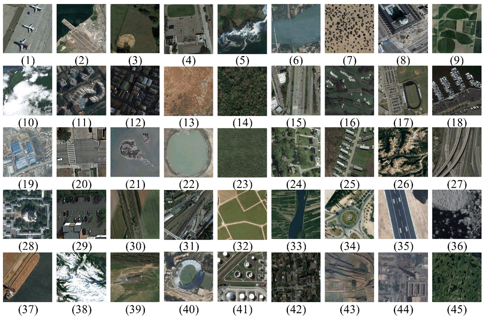
• NWPU-RESISC45 dataset was released by Northwestern Polytechnical University in 2017 and is the largest and most challenging dataset for RSISC task. It contains 31,500 images extracted from Google Earth with a fixed size of 256 × 256 and has 45 scene categories with 700 images in each category The 45 categories are airplane, airport, baseball diamond, basketball court, beach, bridge, chaparral, church, circular farmland, cloud, commercial area, dense residential, desert, forest, freeway, golf course, ground track field, harbor, industrial area, intersection, island, lake, meadow, medium residential, mobile home park, mountain, overpass, palace, parking lot, railway, railway station, rectangular farmland, river, roundabout, runway, sea ice, ship, snowberg, sparse residential, stadium, storage tank, tennis court, terrace, thermal power station, and wetland. Some examples images from the NWPU-RESISC45 dataset are shown in Figure 4.

• UC Merced Land-Use dataset was released by University of California, Merced in 2010 and is the most widely used dataset for RSISC tasks. It contains 2100 RS images of 256 × 256 pixels extracted from USGS National Map Urban Area Imagery collection and has 21 categories with 100 images per category. The 21 categories are agricultural, airplane, baseball diamond, beach, buildings, chaparral, dense residential, forest, freeway, golf course, harbor, intersection, medium residential, mobile home park, overpass, parking lot, river, runway, sparse residential, storage tanks and tennis court. Some example images from the UC Merced Land-Use dataset are shown in Figure 5.

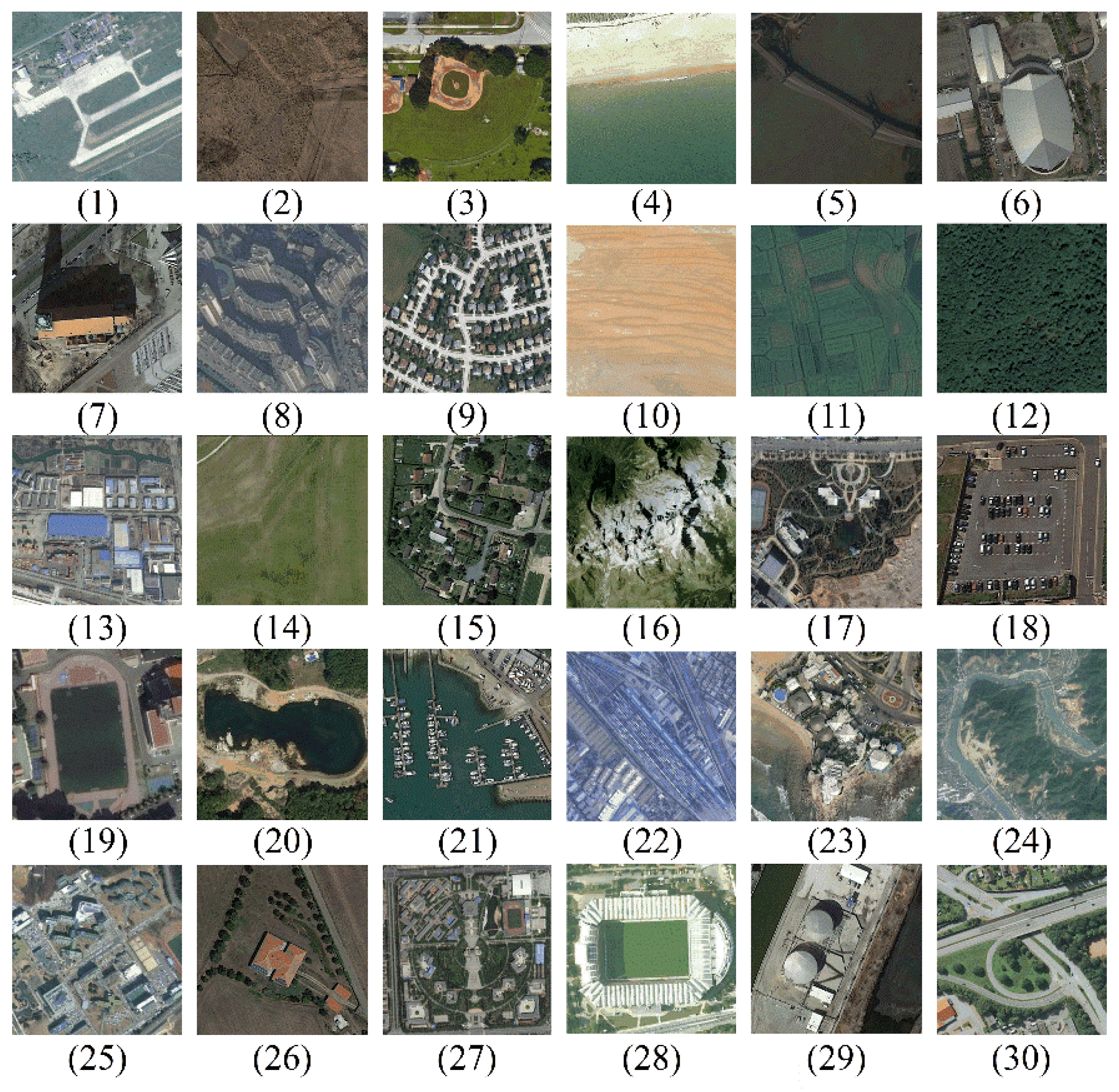
• AID dataset was released by Wuhan University in 2017 and is one of the most complex datasets for RSISC tasks due to the images being extracted from different sensors and their pixel resolution varying from 8 m to 0.5 m. It contains 10,000 RS images of 600 × 600 pixels extracted from Google Earth imagery and has 30 scene categories with about 220 to 400 images per category. The 30 categories are airport, bareland, baseball field, beach, bridge, center, church, commercial, dense residential, desert, farmland, forest, industrial, meadow, medium residential, mountain, parking, park, playground, pond, port, railway station, resort, river, school, sparse residential, square, stadium, storage tanks and viaduct. Some example images from the AID dataset are shown in Figure 6.

3.1.2. Mask Datasets

A RS image with defects is simulated through a Hadamard product of a binary mask and a GT image. The masks of periodical stripes and random noises are randomly generated with Python. The masks of thick cloud are extracted from the NVIDIA Irregular Mask dataset [43]. All the three mask datasets have 2000 images with a 20~30% hole-to-image area ratio. Some example images from the three mask datasets are shown in Figure 7.

3.2. Training Details

3.2.1. Environments

The experiments are carried out on two NVIDIA RTX Titian 24G GPUs with Ubuntu 18.04, Pytorch 1.6.0 and CUDA 10.1. The LPIN is optimized by ADAM optimizer with a learning rate of 0.002. All training images are cropped and resized to 3 × 256 × 256 pixels. The Pytorch DistributedDataParallel API for multi-GPU training and the NVIDIA Apex tool for mixed precision are used to accelerate the training process.

3.2.2. Training Flow

The NWPU-RSISC45 dataset is randomly divided into two parts: 20% for training (6300 images) and the remaining 80% for testing (25,200 images), which means the training ratio is 20%. The training data is then augmented six times by rotating them by 90°, 180°, 270° and flipping them horizontally and vertically, i.e., we use 37,800 images for training. In the training phase, LPIN samples minibatch images $I_0$ from the augmented training dataset and normalize them using the mean and standard deviation of ImageNet. Then, LPIN samples minibatch binary masks $M$ from the mask dataset and perform a Hadamard product of $I_0$ and $M$ to get the RS images with defects, namely the input images $I_{in}$. The RIU of each stage inpaints the defects progressively and the final RIU outputs the inpainting result of LPIN $I_{out}$. Finally, the loss functions are used to restrict the value of $I_{out}$ on a pixel and semantic level. The detailed inpainting training flow is formally presented in Algorithm 1.

Algorithm 1. The training process of LPIN.

$1: I_{in}$ is the input of LPIN,

$2: I_{out}\hspace{1em}$ is the output of LPIN,

$3: f_i$ is the i-th RIU,

$4: x_i^{in}$ is the input of the i-th RIU,

$5: x_i^{res}$ is the residual output of the i-th RIU,

$6: x_i^{out}$ is the output of the i-th RIU.7: for number of max epochs do:

$8: \mathrm{sample} \mathrm{minibatch} \mathrm{of} \mathrm{k} \mathrm{images} \mathrm{from} \mathrm{training} \mathrm{dataset}: I_0=\left\{I_0^1,I_0^2,I_0^3\cdots I_0^k\right\}$

$9: \mathrm{sample} \mathrm{minibatch} \mathrm{of} \mathrm{k} 256\times 256 \mathrm{binary} \mathrm{masks}: M=\left\{M^1,M^2,M^3\cdots M^k\right\}$

$10: \mathrm{generate} \mathrm{input} \mathrm{images}: I_{in}=M⨀I_0$

$11: \mathrm{calculate} \mathrm{the} \mathrm{input} \mathrm{of} \mathrm{first} \mathrm{RIU}: x_0^{in}=concat\left(I_{in},I_{in}\right)$

12:        for number N of phases do:

$13:\hspace{1em}\hspace{1em}{x}_i^{res}=f_i\left(x_i^{in}\right)$

$14:\hspace{1em}\hspace{1em}{x}_i^{out}=x_i^{res}+I_{in}$

$15:\hspace{1em}\hspace{1em}{x}_{i+1}^{in}=cat\left(x_i^{out},I_{in}\right)$

16:        end for

$17: \mathrm{calculate} \mathrm{the} \mathrm{out} \mathrm{of} \mathrm{last} \mathrm{RIU}: I_{out}=x_N^{out}$

18: calculate loss functions.

19: update parameters using ADAM optimizer.

20: end for

Meanwhile, we choose six existing RSISC methods and train them on the same training dataset. Then, the GT images and the images with defects are sent to each RSISC method, as well as the proposed methods which combine the LPIN with RSISC methods to test their classification accuracy, as shown in Figure 8.

3.3. Hyper-Parameters Tuning

3.3.1. Weight Value of Loss Term

$L_{def}$, $L_{val}$, $L_{cnt}$, and $L_{style}$ are used to train the network separately and their values roughly converge to the following numbers: 3 × 10⁻², 1 × 10⁻⁴, 2, and 7 × 10⁻⁵, respectively, as shown in Figure 9. The $L_{tv}$ is not involved in the training, and its rough value is calculated at the start of training, being 2 × 10⁻¹. In order to prevent certain loss from having more impact on the training process than the others, each loss value is scaled to the same order of magnitude by multiplying their weights. Thus, the weight values are preliminary set as: ${\lambda }_{def}=0.6$, ${\lambda }_{val}=160$, ${\lambda }_{cnt}=0.01$, ${\lambda }_{style}=280$, and ${\lambda }_{tv}=0.08$. For the reconstruction loss, considering that the defect regions are expected to have a better inpainting performance than that of the valid regions, we properly increase the number of ${\lambda }_{hole}$ and decrease the number of ${\lambda }_{valid}$. Then we randomly select 450 images from the NWPU-RSISC45 dataset with 10 images per category and conduct a random searching test on them. The final weights are acquired from the test as follows: ${\lambda }_{def}=20$, ${\lambda }_{val}=10$, ${\lambda }_{cnt}=0.05$, ${\lambda }_{style}=100$ and ${\lambda }_{tv}=0.1$.

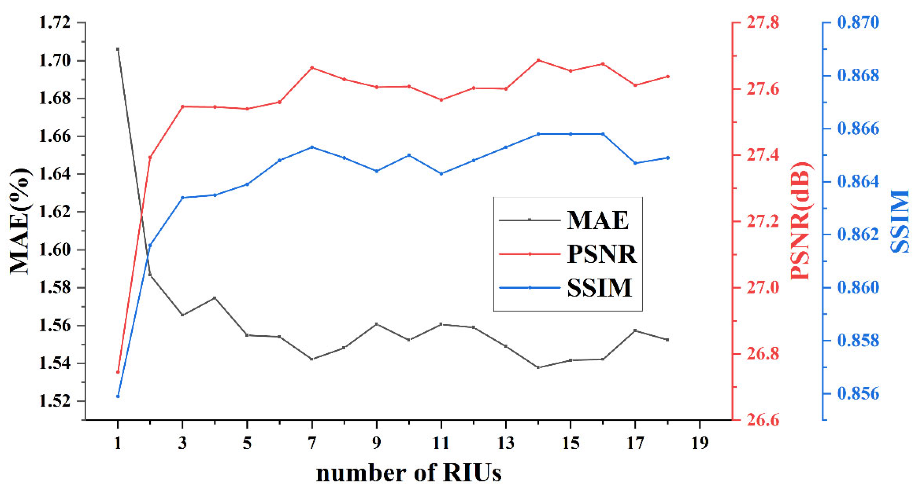
3.3.2. Number of RIUs in LPIN

Too few RIUs may lead to insufficient inpainting capability, while too many RIUs may cause network redundancy and do not improve the performance. Therefore, the number of RIUs need to be determined properly before training. To find the optimal number, tests on LPIN with different RIU numbers are conducted. The Mean Absolute Error (MAE), Peak Signal-to-Noise Ratio (PSNR), and SSIM are used to evaluate the inpainting performance. Among them, the SSIM index has been described in Section 2.3.1. MAE (also known as L1 error) is an index to compare the L1 distance of two images $x$ and $y$, formulated as:

$$MAE\left(x,y\right)=\frac{1}{N}{\displaystyle \sum }_{i=1}^N\left|x^{\left(i\right)}-y^{\left(i\right)}\right|$$

(17)

where $i$ is the pixel value in each image. The lower MAE is, the more similar two images are.

PSNR is one of the most widely used image evaluation indexes, which is calculated as:

$$PSNR\left(x,y\right)=10{\log }_{10}\frac{MA{X}_I^2}{MSE\left(x,y\right)}$$

(18)

where $MSE\left(x,y\right)$ is the L2 distance of $x$ and $y$, $MA{X}_I$ is the maximum pixel value of an image, which is 255 for images in this paper. The larger PSNR is, the more realistic the inpainted image is.

The tests are carried out on multiple LPINs with RIU number changing from one to eighteen. Each test runs for 20 epochs and the inpainting results are show in Figure 10. We can see that the inpainting performance improves at first, but hardly gets better after 8 RIUs. The LPIN with 8 RIUs performs a little inferior to the LPIN with 7 RIUs which reaches its bottleneck. Thus, we set the number of RIU as 7 in the following experiments.

3.4. Image Inpainting Results

We compare our LPIN with 4 state-of-the-art semantic inpainting models: PGN [55], PCONV [43], PRVS [46] and RFR [49]. Each model is trained on the NWPU-RESISC45 dataset under the same condition and inpaints 3 types of defects in RS images: periodic stripes, random noises, and thick clouds (stripes, noises, and clouds for short, respectively).

3.4.1. Model Complexity Analysis

The complexity of the model and parameter is measured by Floating Point Operations (FLOPs) and Bytes. The FLOPs indicates the time consumption of training a model and shows the time complexity of a model. If the FLOPs is too high, the model cannot converge quickly. The Bytes is the number of the parameters and shows the space complexity of a model. The larger the Bytes is, the more data is needed to train a model, which means that the model goes into overfitting easily during training.

The complexity, the model weight and the inpainting speed of our LPIN are compared with other inpainting models and the results are shown in

Table 2. Model Weight and Inpainting Speed of Different Models.

Method	PGN [55]	PCONV [43]	PRVS [46]	RFR [49]	LPIN (Ours)
FLOPs (G)	77.64	18.95	19.71	206.11	6.23
Bytes (M)	249.39	51.55	22.38	30.59	0.095
Model Weight (MB)	3132.8	412.5	666.7	374.8	1.2
Inpainting Speed (fps)	24.89	66.75	22.47	15.75	67.29

. The model complexity is calculated by the Pytorch Torchstat API. We can see that due to the lightweight design, i.e., the multi-stage network of LPIN, the concise architecture of RIU, and the weight sharing strategy, the proposed LPIN has the least model complexity, number of parameters and model weight as well as the fastest inpainting speed.

3.4.2. Quantitative Results

MAE, PSNR and SSIM indexes are used for quantitative comparison as shown in

Table 3. Quantitative inpainting results of different methods.

Method	Stripe Defects			Noise Defects			Cloud Defects
	$\mathbf{M}\mathbf{A}{\mathbf{E}}^{-}(\%)$	$\mathbf{P}\mathbf{S}\mathbf{N}{\mathbf{R}}^{+}\left(\mathbf{dB}\right)$	$\mathbf{S}\mathbf{S}\mathbf{I}{\mathbf{M}}^{+}$	$\mathbf{M}\mathbf{A}{\mathbf{E}}^{-}(\%)$	$\mathbf{P}\mathbf{S}\mathbf{N}{\mathbf{R}}^{+}\left(\mathbf{dB}\right)$	$\mathbf{S}\mathbf{S}\mathbf{I}{\mathbf{M}}^{+}$	$\mathbf{M}\mathbf{A}{\mathbf{E}}^{-}(\%)$	$\mathbf{P}\mathbf{S}\mathbf{N}{\mathbf{R}}^{+}\left(\mathbf{dB}\right)$	$\mathbf{S}\mathbf{S}\mathbf{I}{\mathbf{M}}^{+}$
PCGN [55]	1.737	29.082	0.921	2.548	27.066	0.812	1.873	28.320	0.875
PCONV [43]	1.483	27.621	0.874	2.709	23.555	0.665	1.484	28.092	0.873
PRVS [46]	1.404	28.306	0.883	1.375	28.302	0.882	1.380	28.267	0.882
RFR [49]	1.461	28.897	0.851	1.588	26.794	0.877	1.386	28.421	0.883
LPIN (ours)	0.722	33.849	0.967	0.646	33.282	0.951	1.384	28.432	0.884

$-$ lower is better. $+$ Higher is better.

. As can be seen, the LPIN has a good performance on stripes and noises inpainting and achieves a much better result than the other inpainting models. Its inpainting results for clouds are, however, slightly inferior to the former two. This is because that the LPIN is a lightweight network and has the advantage of inpainting the structured defects rather than the defects with large holes.

3.4.3. Qualitative Comparisons

The inpainting results of three types of defects are shown in Figure 11. The details in the blue box on each image are magnified and shown in the red box. We can see from the figure that despite the small parameter weight, the LPIN achieves a good visual inpainting performance on images with defects. Although the LPIN is inferior to PRVS in MAE for the thick cloud inpainting, there is no significant visual difference.

3.5. Scene Classification Results

The previous section has proven effectiveness of the LPIN in inpainting three types of defects. In this section, scene classification tests are carried out to verify the robustness improvement of the RSISC tasks with the proposed method. The GT images and the corresponding images with defects are sent to six existing RSISC methods and the proposed combined methods respectively to test the classification accuracy. Considering that most RSISC methods are not publicly available, we choose three classical CNN classification networks: VGG16 [56], ResNet50 [61], and Inception V3 [62] and train them on the dataset using the pre-trained weights on ImageNet. In addition, we also use three other models published by our team: HCV + FV [4], ADFF [12], and F²BRBM [16]. The tests are conducted on the NWPU-RESISC45 dataset with a training ratio of 20%, and the final results are calculated by the mean and standard deviation of 10 random repeated experiments.

3.5.1. Classification Accuracy Results

Three measurements are used to evaluate the classification accuracy and robustness improvement of RSISC as follows: (1) Overall accuracy (OA), which is defined as the ratio of the number of correctly classified images to the total number of images. (2) Defect-to-GT Ratio (D2GR), which is a robustness index and represents the ratio of the OA of images with defects to the OA of GT images. The more robust a RSISC method is, the higher D2GR is. (3) Confusion matrix, also known as the error matrix, is used to visualize the classification results of specific categories. In an ideal confusion matrix, all classification results are distributed only on the diagonal. The OA and D2GR of six existing RSISC methods and the corresponding combined methods with LPIN are shown in

Table 4. OA (%) and DR (%) of Six Classifiers and Corresponding Combined Methods with LPIN on NWPU-RSISC45 Dataset.

Method	GT OA	Stripe Defects		Noise Defects		Cloud Defects
		OA	D2GR	OA	D2GR	OA	D2GR
HCV + FV [4]	82.36 ± 0.17	32.48 ± 0.43	39.44	39.15 ± 0.27	47.54	50.12 ± 0.44	60.85
HCV + FV + LPIN		82.15 ± 0.23	99.77	80.94 ± 0.14	98.30	79.42 ± 0.34	96.45
ADFF [12]	88.82 ± 0.22	43.17 ± 0.57	48.60	53.80 ± 0.38	60.57	49.74 ± 0.39	56.00
ADFF + LPIN		88.23 ± 0.25	99.37	87.35 ± 0.28	98.37	83.63 ± 0.34	94.19
VGG16 [56]	87.66 ± 0.37	28.01 ± 0.53	31.95	28.53 ± 0.41	32.55	39.50 ± 0.55	45.06
VGG16 + LPIN		87.21 ± 0.39	99.61	86.05 ± 0.36	98.29	82.82 ± 0.41	94.60
ResNet50 [61]	90.12 ± 0.14	36.80 ± 0.51	40.83	48.17 ± 0.53	53.45	50.45 ± 0.61	55.98
ResNet50+LPIN		89.98±0.44	99.85	89.66 ± 0.49	99.50	87.75 ± 0.51	97.38
Inception V3 [62]	93.42 ± 0.39	42.17 ± 0.69	45.14	56.61 ± 0.87	60.60	52.99 ± 0.75	56.72
Inception V3 + LPIN		93.30 ± 0.51	99.90	92.99 ± 0.62	99.57	88.45 ± 0.62	94.71
F2BRBM [16]	94.72 ± 0.38	44.16 ± 0.45	46.62	43.36 ± 0.32	45.78	60.80 ± 0.41	64.19
F2BRBM + LPIN		93.77 ± 0.37	99.00	94.43 ± 0.38	99.69	89.92 ± 0.38	94.93

. We can see that the OA of original RSISC methods decrease dramatically on the images with defects, while the proposed methods still have a good performance. Specifically speaking, they generally achieve an D2GR of around 99% for periodic stripe defects and random noise defects and around 95% for thick cloud defects, which proves a great improvement on the robustness of RSISC.

The confusion matrix of original F²BRBM on GT images is shown in Figure 12, and that of original F²BRBM and the corresponding combined method F²BRBM + LPIN on images with defects are show in Figure 13. It can be seen from the left column in Figure 13 that defects of all 3 types cause a large number of confusing items for the original F²BRBM. This is due to the defects cutting off the continuous semantic information of RS images and F²BRBM only being able to classify images depending on the backgrounds. As Figure 14 shows, some defects images from two different categories have much similar backgrounds which subsequently causes misclassification. For example, 25.9% of the airport images with stripe defects are classified to railway stations, 69.4% of the circular farmland images with noise defects are classified to rectangular farmlands and 39.2% of the desert images with cloud defects are classified to lakes.

The LPIN eliminates the semantic irrelevant defects, generates pixels that has contextual semantic information, improves semantic coherence, provides more information for F2BRBM, and thus increases the classification accuracy. According to the right column of Figure 13, the classification accuracy of airports with stripe defects, circular farmlands with noise defects and deserts with cloud defects increase to 91.4%, 97.0% and 97.7%, respectively. It is also worth noting that the LPIN would not bring additional semantic information, therefore, the accuracy of categories that are apt to be misclassified originally is not improved too much. For example, the original F²BRBM has a 15.2% probability of misclassifying palaces into churches on the GT images, and the combined method still has a 15.7% misclassifying probability on the images with stripe defects.

3.5.2. OA Comparison of Different Inpainting Models

The OA results on images with defects of the original F²BRBM combined with different inpainting models are shown in

Table 5. OA Comparison of F2BRBM Combined with Different Inpainting Models on Images with Defects.

Method	Stripes Defects	Noises Defects	Clouds Defects
F2BRBM + PGN [55]	93.06 ± 0.22	85.43 ± 0.20	86.49 ± 0.19
F2BRBM + PCONV [43]	79.84 ± 0.89	60.60 ± 1.25	89.01 ± 0.15
F2BRBM + PRVS [46]	92.93 ± 0.18	92.81 ± 0.43	89.99 ± 0.34
F2BRBM + RFR [49]	66.43 ± 1.05	74.23 ± 0.92	90.19 ± 0.27
F2BRBM + LPIN (ours)	93.77 ± 0.23	94.43 ± 0.15	89.92 ± 0.25

and Figure 15. We can see that the LPIN performs better than the other inpainting models on images with stripe and noise defects, but sightly inferior to PRVS and RFR on images with cloud defects. The LPIN strengthens the utilization of image contextual information through residual architecture and the multiple accesses of the input images. Stripe and noise defects are small and scattered. They cut off continuous semantic information but retain the global content and local contextual information. Therefore, LPIN performs well when processing images with small and scattered defects. In contrast, the cloud defects are relatively large and concentrated defects. The images with cloud defects lose contextual information and the inpainting model needs to have a more comprehensive understanding of the local semantic information to classify them correctly. Therefore, the inpainting performance of LPIN for images with large and concentrated defects is not as good as the one for images with stripe and noise defects, and the improvement of classification accuracy is not as obvious as the other two.

4. Discussion

4.1. Generalization Ability Results of Different Datasets

The LPIN trained on NWPU-RSISC45 dataset are directly applied to UC Merced land-use dataset and AID dataset to test the generalization ability of the proposed method. The inpainting results are shown in

Table 6. Quantitative Inpainting Results of UC Merced Land-use Dataset and AID Dataset.

Dataset	Stripes Defects		Noises Defects			Clouds Defects
	$\mathbf{M}\mathbf{A}{\mathbf{E}}^{-}$ (%)	$$\begin{gathered} \mathbf{P}\mathbf{S}\mathbf{N}{\mathbf{R}}^{+} \\ \left(\mathbf{dB}\right) \end{gathered}$$	$\mathbf{S}\mathbf{S}\mathbf{I}{\mathbf{M}}^{+}$	$$\begin{gathered} \mathbf{M}\mathbf{A}{\mathbf{E}}^{-} \\ (\%) \end{gathered}$$	$$\begin{gathered} \mathbf{P}\mathbf{S}\mathbf{N}{\mathbf{R}}^{+} \\ \left(\mathbf{dB}\right) \end{gathered}$$	$\mathbf{S}\mathbf{S}\mathbf{I}{\mathbf{M}}^{+}$	$$\begin{gathered} \mathbf{M}\mathbf{A}{\mathbf{E}}^{-} \\ (\%) \end{gathered}$$	$$\begin{gathered} \mathbf{P}\mathbf{S}\mathbf{N}{\mathbf{R}}^{+} \\ \left(\mathbf{dB}\right) \end{gathered}$$	$\mathbf{S}\mathbf{S}\mathbf{I}{\mathbf{M}}^{+}$
UC Merced Land-Use	0.776	33.589	0.964	0.880	30.958	0.911	1.616	27.049	0.885
AID	0.711	34.062	0.965	0.666	33.122	0.942	1.395	28.419	0.889

$-$ lower is better. $+$ Higher is better.

and Figure 16. The OA and D2GR of F²BRBM and the corresponding combined method F²BRBM + LPIN on these two datasets are calculated as shown in

Table 7. OA (%) and ROR (%) of F2BRBM and F2BRBM + LPIN on UC Merced Land-use Dataset and AID Dataset.

Dataset	Method	GT OA	Stripe Defects		Noise Defects		Cloud Defects
			OA	D2GR	OA	D2GR	OA	D2GR
UC Merced Land-Use	F2BRBM	97.23 ± 0.03	48.76 ± 0.26	50.15	70.71 ± 0.32	72.72	72.63 ± 0.28	74.70
	F2BRBM + LPIN		96.56 ± 0.14	99.31	94.39 ± 0.12	97.08	93.24 ± 0.09	95.90
AID	F2BRBM	96.05 ± 0.02	44.34 ± 0.12	46.16	35.08 ± 0.27	36.52	60.88 ± 0.30	60.38
	F2BRBM + LPIN		94.05 ± 0.22	97.92	91.76 ± 0.19	95.53	89.23 ± 0.42	93.00

and Figure 17.

We can see that the LPIN still has a good inpainting performance, and the combined method with LPIN can correct most misclassified items. It can reach a high level of D2GR on different datasets with defects, and significantly increase the robustness of RSISC, which proves a good generalization ability of the proposed method.

4.2. Image Inpainting Ablation Studies

In this section, several ablation tests of the network architecture and the loss functions are carried out to analyze their influence on inpainted image quality. Each test is trained on NWPU RSISC-45 dataset for 20 epochs.

4.2.1. Network Architecture: With vs. without LSTM

The multi-stage network LPIN can be regarded as a time series structure. Due to the good performance of Long Short-Term Memory (LSTM) [63] on time series prediction [7], we adopt LSTM in LPIN and try to strengthen the inner connection between different RIU stages. The results are shown as

Table 8. Inpainting Quality Comparison of LPIN with or without LSTM.

Network Architecture		With LSTM	Without LSTM
Stripe defects	${MAE}^{-}$(%)	2.786	1.015
	${PSNR}^{+}$(dB)	22.048	31.193
	${SSIM}^{+}$	0.785	0.935
Noise defects	${MAE}^{-}$(%)	2.774	2.330
	${PSNR}^{+}$(dB)	23.131	24.690
	${SSIM}^{+}$	0.664	0.715
Cloud defects	${MAE}^{-}$(%)	2.908	1.630
	${PSNR}^{+}$(dB)	21.751	26.885
	${SSIM}^{+}$	0.825	0.875

$-$ lower is better. $+$ Higher is better.

, from which we can see that the inpainted image quality for LPIN with LSTM is worse than that for LPIN without LSTM.

Although LSTM provides extra transmission of image features among RIUs, it increases the network weights. As a result, the number of its parameters exceeds that of the LPIN main body, which lowers the parameter gradient updating efficiency of image inpainting.

4.2.2. Reconstruction Loss: L1 vs. Negative SSIM

L1 and negative SSIM are two commonly used reconstruction losses for constraining two images. The results of LPIN with L1 or with negative SSIM are shown in

Table 9. Inpainting Quality Comparison of Different Reconstruction Loss.

Reconstruction Loss		L1 Loss	Negative SSIM Loss
Stripe defects	${MAE}^{-}$(%)	1.400	1.015
	${PSNR}^{+}$(dB)	28.989	31.193
	${SSIM}^{+}$	0.887	0.935
Noise defects	${MAE}^{-}$(%)	2.780	2.330
	${PSNR}^{+}$(dB)	23.329	24.690
	${SSIM}^{+}$	0.656	0.715
Cloud defects	${MAE}^{-}$(%)	1.664	1.630
	${PSNR}^{+}$(dB)	27.053	26.885
	${SSIM}^{+}$	0.867	0.875

$-$ lower is better. $+$ Higher is better.

. We can see that LPIN with negative SSIM loss achieves better inpainting quality. The L1 loss constrains two images pixel by pixel, therefore, if two images only have a slight difference in brightness, their L1 distance might be very large. The negative SSIM overcomes this drawback by measuring the differences in brightness, contrast and structure of two images, which makes it a more effective reconstruction loss function.

4.2.3. Feature Extractor: ResNet50 vs. VGG16

VGG16 and ResNet50 are two well-performed feature extractors [23]. Different features extracted from them are used to calculate the content and style loss and compare the inpainting results, which are shown in

Table 10. Inpainting Quality Comparison of ResNet50 and VGG16 Extractor.

Feature Extractor		ResNet50	VGG16
Stripe defects	${MAE}^{-}$(%)	1.356	1.357
	${PSNR}^{+}$(dB)	30.978	30.912
	${SSIM}^{+}$	0.903	0.910
Noise defects	${MAE}^{-}$(%)	2.403	2.418
	${PSNR}^{+}$(dB)	24.715	24.841
	${SSIM}^{+}$	0.767	0.761
Cloud defects	${MAE}^{-}$(%)	1.710	1.671
	${PSNR}^{+}$(dB)	26.554	26.715
	${SSIM}^{+}$	0.852	0.849

$-$ lower is better. $+$ Higher is better.

. It can be seen that there is little difference between the two extractors in inpainting quality. We believe that ResNet50 pays more attention to the low-level features, which are extracted from the last few layers of the network and are useless for LPIN, since our network needs the high-level semantic features, which are extracted from the first several layers. Besides, VGG16 has a simpler structure and smaller convolution filter for the first several layers than ResNet50. As a result, we choose VGG16 as our feature extractor.

4.2.4. Feature Extractor Layer: Maxpooling vs. Convolution

The convolution layer and the maxpooling layer of VGG16 can both extract image features. A test on two different layers is carried out and the results are shown in

Table 11. Inpainting Quality Comparison of Different Extractor Layers.

Feature Extractor Layer		Maxpooling	Convolution
Stripe defects	${MAE}^{-}$(%)	1.063	1.015
	${PSNR}^{+}$(dB)	30.834	31.193
	${SSIM}^{+}$	0.930	0.935
Noise defects	${MAE}^{-}$(%)	2.987	2.330
	${PSNR}^{+}$(dB)	22.748	24.690
	${SSIM}^{+}$	0.636	0.715
Cloud defects	${MAE}^{-}$(%)	1.654	1.630
	${PSNR}^{+}$(dB)	26.453	26.885
	${SSIM}^{+}$	0.875	0.875

$-$ lower is better. $+$ Higher is better.

. It can be seen that the convolution layer gives a slightly better inpainting result. We speculate that partial pixels of the feature are discarded when passing through the maxpooling layer. Therefore, some effective information cannot be transmitted to the extractor. As a result, we choose the convolution layers to extract image features.

4.3. Inpainting Results of Images with Hybrid Defecs

It is not always the case that only one type of defect exists on real RS images. Sometimes several types of defects appear on an image at the same time. Therefore, a test of images with a combined defects is also conducted. The quantitative image inpainting results are shown in

Table 12. Inpainting Quality on NWPU-RSISC45 Dataset with Combined Defects.

Defect Type	$\mathbf{M}\mathbf{A}{\mathbf{E}}^{-}(\%)$	$\mathbf{P}\mathbf{S}\mathbf{N}{\mathbf{R}}^{+}\left(\mathbf{dB}\right)$	$\mathbf{S}\mathbf{S}\mathbf{I}{\mathbf{M}}^{+}$
Stripes + noises	1.255	30.824	0.928
Stripes + clouds	2.014	26.883	0.855
Noises + clouds	1.927	26.847	0.846
Stripes + noises + clouds	2.456	26.075	0.822

$-$ lower is better. $+$ Higher is better.

and qualitative visual results are shown in Figure 18.

The OA and D2GR of F²BRBM method and the corresponding combined method F²BRBM+LPIN on NWPU-RSISC45 dataset with combined defects are shown in

Table 13. OA (%) and D2GR (%) of F2BRBM and F2BRBM+LPIN on NWPU-RSISC45 Dataset with Combined Defects.

Defect Type	Methods	GT OA	OA	D2GR
Stripes + Noises	F2BRBM	94.72 ± 0.38	30.17 ± 0.44	31.85
	F2BRBM + LPIN		93.97 ± 0.28	99.21
Stripes + clouds	F2BRBM		19.18 ± 0.82	20.25
	F2BRBM + LPIN		87.66 ± 0.52	92.55
Noises + clouds	F2BRBM		19.75 ± 0.76	20.85
	F2BRBM + LPIN		87.16 ± 0.35	92.02
Stripes + noises + clouds	F2BRBM		9.67 ± 0.68	10.21
	F2BRBM + LPIN		84.99 ± 0.48	89.73

. We can see that the OA of original F²BRBM decreases dramatically to only around 9%, but the proposed combined method still has a D2GR of around 90%, which proves its great robustness. The corresponding confusion matrixes of these two methods on images with defects of all 3 types are shown in Figure 19.

As Figure 19a shows, many defect RS images are misclassified mainly into three categories: chaparral, harbor and parking lot, which all have scattered features, i.e., the scattered trees in a chaparral, the scattered ships in a harbor and the scattered vehicles in a parking lot. As Figure 20a shows, we believe that the combination of three defects added many scatted patches to the RS images and makes them visually similar to the three misclassified categories. Therefore, the misclassification mainly happens in these three categories. According to the confusion matrix of Figure 19a, 51.5% of the church images are classified into parking lots, 48.7% of the beach images are classified into harbors, and 68.9% of the wetland images are classified into chaparrals. However, with the help of the LPIN, the scattered disturbed patches are inpainted and the classification accuracy are improved correspondingly as Figure 20b shows. According to Figure 19b, the classification accuracy of churches, beaches and wetlands is 80.1%, 96.1% and 82.5%, respectively.

5. Conclusions

In this paper, a progressive lightweight inpainting network named LPIN is proposed to provide a purified input for the RSISC method. Compared with other state-of-the-art inpainting networks, the LPIN can achieve a better inpainting performance with a simpler structure, a lighter weight of only 1.2 MB and a faster inpainting speed of 67.29 fps, which makes it possible to implant to small portable devices. The LPIN is then combined with the existing RSISC method to form a combined classification approach, which can effectively improve the classification accuracy of the existing classification methods on images with defects. It keeps the comparable classification accuracy level on RS images with defects as that without defects, thus improving the robustness of high-resolution RSISC tasks. Experimental results on different datasets prove that the proposed method also has a good generalization ability.

There are mainly three limitations in our work. Firstly, the RS images of a fixed region can be captured by satellites multiple times and thus they not only have spatial information but also temporal information. However, we focus on single RS image inpainting and only use its spatial information in this work. Secondly, it takes lots of effort to acquire the RS images with defects from satellites, therefore we only train and test our LPIN on the standard datasets. Finally, as the image inpainting network needs to acquire the global semantic and local contextual information of an image, the LPIN requires larger datasets and more training iterations compared with other types of networks such as image classification.

In our following work, we plan to carry out image inpainting research using the history RS images with temporal information, obtain real RS images from satellites, adopt more deep learning regularization techniques in the training process—such as early stopping [23] which we believe can reduce overfitting—and enhance the generalization ability of our model and further lower the time consumption.

References

1. Cheng, G.; Xie, X.; Han, J.; Guo, L.; Xia, G.S. Remote Sensing Image Scene Classification Meets Deep Learning: Challenges, Methods, Benchmarks, and Opportunities. IEEE J. Sel. Topics Appl. Earth Observ. Remote Sens. 2020, 13, 3735–3756. [Google Scholar] [CrossRef]
2. Yang, Y.; Newsam, S. Bag-of-visual-words and spatial extensions for land-use classification. In Proceedings of the 18th SIGSPATIAL International Conference on Advances in Geographic Information Systems, San Jose, CA, USA, 3–5 November 2010; pp. 270–279. [Google Scholar]
3. Jiang, Y.; Yuan, J.; Yu, G. Randomized spatial partition for scene recognition. In Proceedings of the European Conference on Computer Vision (ECCV), Florence, Italy, 7–13 October 2012; pp. 730–743. [Google Scholar]
4. Wu, H.; Liu, B.; Su, W.; Zhang, W.; Sun, J. Hierarchical coding vectors for scene level land-use classification. Remote Sens. 2016, 8, 436. [Google Scholar] [CrossRef] [Green Version]
5. Wu, H.; Liu, B.; Su, W.; Zhang, W.; Sun, J. Deep filter banks for land-use scene classification. IEEE Geosci. Remote Sens. Lett. 2016, 13, 1895–1899. [Google Scholar] [CrossRef]
6. Mustaqeem; Kwon, S. Att-net: Enhanced emotion recognition system using lightweight self-attention module. Appl. Soft Comput. 2021, 102, 107101. [Google Scholar] [CrossRef]
7. Muhammad, K.; Mustaqeem; Ullah, A.; Imran, A.S.; Sajjad, M.; Kiran, M.S.; Sannino, G.; de Albuquerque, V.H.C. Human action recognition using attention based LSTM network with dilated cnn features. Future Gener. Comput. Syst. 2021, 125, 820–830. [Google Scholar] [CrossRef]
8. Lee, H.; Kwon, H. Contextual deep CNN based hyperspectral classification. In Proceedings of the 2016 IEEE International Geoscience and Remote Sensing Symposium (IGARSS), Beijing, China, 10–15 July 2016; pp. 3322–3325. [Google Scholar]
9. Hu, F.; Xia, G.S.; Hu, J.; Zhang, L. Transferring deep convolutional neural networks for the scene classification of high-resolution remote sensing imagery. Remote Sens. 2015, 7, 14680–14707. [Google Scholar] [CrossRef] [Green Version]
10. Du, P.; Li, E.; Xia, J.; Samat, A.; Bai, X. Feature and model level fusion of pretrained CNN for remote sensing scene classification. IEEE J. Sel. Topics Appl. Earth Observ. Remote Sens. 2019, 12, 2600–2611. [Google Scholar] [CrossRef]
11. Yin, L.; Yang, P.; Mao, K.; Liu, Q. Remote Sensing Image Scene Classification Based on Fusion Method. J. Sens. 2021, 2021, 6659831. [Google Scholar] [CrossRef]
12. Li, B.; Su, W.; Wu, H.; Li, R.; Zhang, W.; Qin, W.; Zhang, S. Aggregated deep Fisher feature for VHR remote sensing scene classification. IEEE J. Sel. Top. Appl. Earth Obs. Remote Sens. 2019, 12, 3508–3523. [Google Scholar] [CrossRef]
13. Wang, Q.; Liu, S.; Chanussot, J.; Li, X. Scene classification with recurrent attention of VHR remote sensing images. IEEE Trans. Geosci. Remote Sens. 2019, 57, 1155–1167. [Google Scholar] [CrossRef]
14. Li, H.; Wang, W.; Pan, L.; Li, W.; Du, Q.; Tao, R. Robust capsule network based on maximum correntropy criterion for hyperspectral image classification. IEEE J. Sel. Topics Appl. Earth Observ. Remote Sens. 2020, 13, 738–751. [Google Scholar] [CrossRef]
15. Jiang, X.; Liu, W.; Zhang, Y.; Liu, J.; Li, S.; Lin, J. Spectral–spatial hyperspectral image classification using dual-channel capsule networks. IEEE Geosci. Remote Sens. Lett. 2021, 18, 1094–1098. [Google Scholar] [CrossRef]
16. Zhang, X.; An, W.; Sun, J.; Wu, H.; Zhang, W.; Du, Y. Best representation branch model for remote sensing image scene classification. IEEE J. Sel. Topics Appl. Earth Observ. Remote Sens. 2021, 14, 9768–9780. [Google Scholar] [CrossRef]
17. Hu, W.; Huang, Y.; Wei, L.; Zhang, F.; Li, F. Deep convolutional neural networks for hyperspectral image classification. J. Sens. 2015, 2015, 258619. [Google Scholar] [CrossRef] [Green Version]
18. Li, B.; Su, W.; Wu, H.; Li, R.; Zhang, W.; Qin, W.; Zhang, S.; Wei, J. Further exploring convolutional neural networks’ Potential for Land-Use Scene Classification. IEEE Geosci. Remote Sens. Lett. 2020, 17, 1687–1691. [Google Scholar] [CrossRef]
19. Li, B.; Guo, Y.; Yang, J.; Wang, L.; Wang, Y.; An, W. Gated recurrent multiattention network for VHR remote sensing image classification. IEEE Trans. Geosci. Remote Sens. 2021, 1–13. [Google Scholar] [CrossRef]
20. Cheng, G.; Han, J.; Lu, X. Remote sensing image scene classification: Benchmark and state of the art. Proc. IEEE 2017, 105, 1865–1883. [Google Scholar] [CrossRef] [Green Version]
21. Xia, G.; Hu, J.; Hu, F.; Shi, B.; Bai, X.; Zhong, Y.; Zhang, L.; Lu, X. AID: A benchmark data set for performance evaluation of aerial scene classification. IEEE Trans. Geosci. Remote Sens. 2017, 55, 3965–3981. [Google Scholar] [CrossRef] [Green Version]
22. Helber, P.; Bischke, B.; Dengel, A.; Borth, D. EuroSAT: A Novel Dataset and Deep Learning Benchmark for Land Use and Land Cover Classification. IEEE J. Sel. Top. Appl. Earth Observ. Remote Sens. 2019, 12, 2217–2226. [Google Scholar] [CrossRef] [Green Version]
23. Naushad, R.; Kaur, T.; Ghaderpour, E. Deep Transfer Learning for Land Use and Land Cover Classification: A Comparative Study. Sensors 2021, 21, 8083. [Google Scholar] [CrossRef]
24. Ju, J.; Roy, D.P. The availability of cloud-free Landsat ETM+ data over the conterminous United States and globally. Remote Sens. Environ. 2008, 112, 1196–1211. [Google Scholar] [CrossRef]
25. Li, Q.; Shen, L.; Guo, S.; Lai, Z. Wavelet integrated CNNs for noise-robust image classification. In Proceedings of the 2020 IEEE Conference on Computer Vision and Pattern Recognition (CVPR), Seattle, WA, USA, 13–19 June 2020; pp. 7245–7254. [Google Scholar]
26. Duan, P.; Kang, X.; Li, S.; Ghamisi, P. Noise-robust hyperspectral image classification via multi-scale total variation. IEEE J. Sel. Topics Appl. Earth Observ. Remote Sens. 2019, 12, 1948–1962. [Google Scholar] [CrossRef]
27. Chen, Y.; Das, M. An automated technique for image noise identification using a simple pattern classification approach. In Proceedings of the 50th Midwest Symposium on Circuits and Systems (MWSCAS), Montreal, QC, Canada, 5–8 August 2007; pp. 819–822. [Google Scholar]
28. Chen, C.; Li, W.; Tramel, E.W.; Cui, M.; Prasad, S.; Fowler, J.E. Spectral–spatial preprocessing using multihypothesis prediction for noise-robust hyperspectral image classification. IEEE J. Sel. Topics Appl. Earth Observ. Remote Sens. 2014, 7, 1047–1059. [Google Scholar] [CrossRef]
29. Elharrouss, O.; Almaadeed, N.; Al-Maadeed, S.; Akbari, Y. Image inpainting: A review. Neural Process. Lett. 2020, 51, 2007–2028. [Google Scholar] [CrossRef] [Green Version]
30. Ruzic, T.; Pizurica, A. Context-aware patch-based image inpainting using markov random field modeling. IEEE Trans. Image Process. 2015, 24, 444–456. [Google Scholar] [CrossRef]
31. Jin, K.H.; Ye, J.C. Annihilating filter-based low-rank hankel matrix approach for image inpainting. IEEE Trans. Image Process. 2015, 24, 3498–3511. [Google Scholar]
32. Barnes, C.; Shechtman, E.; Finkelstein, A.; Goldman, D.B. Patchmatch: A randomized correspondence algorithm for structural image editing. ACM Trans. Graph. 2009, 28, 24. [Google Scholar] [CrossRef]
33. Kawai, N.; Sato, T.; Yokoya, N. Dminished reality based on image inpainting considering background geometry. IEEE Trans. Vis. Comput. Graph. 2016, 22, 1236–1247. [Google Scholar] [CrossRef] [Green Version]
34. Zheng, J.; Jiang, J.; Xu, H.; Liu, Z.; Gao, F. Manifold-based nonlocal second-order regularization for hyperspectral image inpainting. IEEE J. Sel. Topics Appl. Earth Observ. Remote Sens. 2020, 14, 224–236. [Google Scholar] [CrossRef]
35. Zhuang, L.; Bioucas-Dias, J.M. Fast hyperspectral image denoising and inpainting based on low-rank and sparse representations. IEEE J. Sel. Topics Appl. Earth Observ. Remote Sens. 2018, 11, 730–742. [Google Scholar] [CrossRef]
36. Li, X.; Shen, H.; Li, H.; Zhang, L. Patch matching-based multitemporal group sparse representation for the missing information reconstruction of remote-sensing images. IEEE J. Sel. Topics Appl. Earth Observ. Remote Sens. 2016, 9, 3629–3641. [Google Scholar] [CrossRef]
37. Lin, C.; Lai, K.; Chen, Z.; Chen, J. Patch-based information reconstruction of cloud-contaminated multitemporal images. IEEE Trans. Geosci. Remote Sens. 2014, 52, 163–174. [Google Scholar] [CrossRef]
38. Pathak, D.; Krahenbuhl, P.; Donahue, J.; Darrell, T.; Efros, A.A. Context Encoders: Feature learning by inpainting. In Proceedings of the 2016 IEEE Conference on Computer Vision and Pattern Recognition (CVPR), Las Vegas, NV, USA, 26–30 June 2016; pp. 2536–2544. [Google Scholar]
39. Goodfellow, I.; Pouget-Abadie, J.; Mirza, M.; Xu, B.; Warde-Farley, D.; Ozair, S.; Courville, A.; Bengio, Y. Generative adversarial nets. In Proceedings of the advances in Neural Information Processing Systems (NeurIPS), Montreal, QC, Canada, 8–13 December 2014; pp. 2672–2680. [Google Scholar]
40. Iizuka, S.; Simo-Serra, E.; Ishikawa, H. Globally and locally consistent image completion. ACM Trans. Graph. 2017, 36, 107. [Google Scholar] [CrossRef]
41. Yu, J.; Lin, Z.; Yang, J.; Shen, X.; Huang, T.S. Generative image inpainting with contextual attention. In Proceedings of the 2018 IEEE Conference on Computer Vision and Pattern Recognition (CVPR), Salt Lake City, UT, USA, 18–23 June 2018; pp. 5505–5514. [Google Scholar]
42. Gulrajani, I.; Ahmed, F.; Arjovsky, M.; Dumoulin, V.; Courville, A.C. Improved training of wasserstein GANs. In Proceedings of the advances in Neural Information Processing Systems (NeurIPS), Long Beach, CA, USA, 4–9 December 2017; pp. 5767–5777. [Google Scholar]
43. Liu, G.; Reda, F.A.; Shih, K.J.; Wang, T.C.; Tao, A.; Catanzaro, B. Image inpainting for irregular holes using partial convolutions. In Proceedings of the European Conference on Computer Vision (ECCV), Munich, Germany, 8–14 September 2018; pp. 89–105. [Google Scholar]
44. Ronneberger, O.; Fischer, P.; Brox, T. U-Net: Convolutional networks for biomedical image segmentation. In Proceedings of the International Conference on Medical Image Computing and Computer-Assisted Intervention (MICCAI), Munich, Germany, 5–9 October 2015; pp. 234–241. [Google Scholar]
45. Yu, J.; Lin, Z.; Yang, J.; Shen, X.; Lu, X.; Huang, T. Free-Form Image Inpainting with Gated Convolution. In Proceedings of the 2019 IEEE International Conference on Computer Vision (ICCV), Seoul, Korea, 27 October–2 November 2019; pp. 4470–4479. [Google Scholar]
46. Li, J.; He, F.; Zhang, L.; Du, B.; Tao, D. Progressive reconstruction of visual structure for image inpainting. In Proceedings of the 2019 IEEE International Conference on Computer Vision (ICCV), Seoul, Korea, 27 October–2 November 2019; pp. 6721–6729. [Google Scholar]
47. Nazeri, K.; Ng, E.; Joseph, T.; Qureshi, F.; Ebrahimi, M. EdgeConnect: Structure guided image inpainting using edge prediction. In Proceedings of the 2019 IEEE International Conference on Computer Vision (ICCV), Seoul, Korea, 27 October–2 November 2019; pp. 3265–3274. [Google Scholar]
48. Liu, H.; Jiang, B.; Xiao, Y.; Yang, C. Coherent semantic attention for image inpainting. In Proceedings of the 2019 IEEE Conference on Computer Vision and Pattern Recognition (CVPR), Seoul, Korea, 15–20 June 2019; pp. 4169–4178. [Google Scholar]
49. Li, J.; Wang, N.; Zhang, L.; Du, B.; Tao, D. Recurrent feature reasoning for image inpainting. In Proceedings of the 202 IEEE Conference on Computer Vision and Pattern Recognition (CVPR), Seattle, WA, USA, 13–19 June 2020; pp. 7757–7765. [Google Scholar]
50. Zhao, L.; Mo, Q.; Lin, S.; Wang, Z.; Lu, D. UCTGAN: Diverse Image Inpainting Based on Unsupervised Cross-Space Translation. In Proceedings of the 2020 IEEE International Conference on Computer Vision (CVPR), Seattle, WA, USA, 13–19 June 2020; pp. 5740–5749. [Google Scholar]
51. Dong, J.; Yin, R.; Sun, X.; Li, Q.; Yang, Y.; Qin, X. Inpainting of remote sensing SST images with deep convolutional generative adversarial network. IEEE Geosci. Remote Sens. Lett. 2019, 16, 173–177. [Google Scholar] [CrossRef]
52. Radford, A.; Metz, L.; Chintala, S. Unsupervised representation learning with deep convolutional generative adversarial networks. arXiv 2015, arXiv:1511.06434. [Google Scholar]
53. Zhang, Q.; Yuan, Q.; Zeng, C.; Li, X.; Wei, Y. Missing data reconstruction in remote sensing image with a unified spatial–temporal–spectral deep convolutional neural network. IEEE Trans. Geosci. Remote Sens. 2018, 56, 4274–4288. [Google Scholar] [CrossRef] [Green Version]
54. Wong, R.; Zhang, Z.; Wang, Y.; Chen, F.; Zeng, D. HSI-IPNet: Hyperspectral imagery inpainting by deep learning with adaptive spectral extraction. IEEE J. Sel. Topics Appl. Earth Observ. Remote Sens. 2020, 13, 4369–4380. [Google Scholar] [CrossRef]
55. Zhang, H.; Hu, Z.; Luo, C.; Zuo, W.; Wang, M. Semantic image inpainting with progressive generative networks. In Proceedings of the 26th ACM International Conference on Multimedia (ACM MM), Seoul, Korea, 22–26 October 2018; pp. 1939–1947. [Google Scholar]
56. Simonyan, K.; Zisserman, A. Very deep convolutional networks for large-scale image recognition. arXiv 2015, arXiv:1409.1556. [Google Scholar]
57. Wang, Z.; Bovik, A.C.; Sheikh, H.R.; Simoncelli, E.P. Image quality assessment: From error visibility to structural similarity. IEEE Trans. Image Process 2004, 13, 600–612. [Google Scholar] [CrossRef] [Green Version]
58. Gatys, L.A.; Ecker, A.S.; Bethge, M. Image style transfer using convolutional neural networks. In Proceedings of the 2016 IEEE Conference on Computer Vision and Pattern Recognition (CVPR), Las Vegas, NV, USA, 26–30 June 2016; pp. 2414–2423. [Google Scholar]
59. Deng, J.; Dong, W.; Socher, R.; Li, L.; Li, K.; Fei-Fei, L. ImageNet: A large-scale hierarchical image database. In Proceedings of the 2009 IEEE Conference on Computer Vision and Pattern Recognition (CVPR), Miami, FL, USA, 20–25 June 2009; pp. 248–255. [Google Scholar]
60. Johnson, J.; Alahi, A.; Fei-Fei, L. Perceptual losses for real-time style transfer and super-resolution. In Proceedings of the European Conference on Computer Vision (ECCV), Amsterdam, The Netherlands, 8–16 October 2016; pp. 694–711. [Google Scholar]
61. He, K.; Zhang, X.; Ren, S.; Sun, J. Deep residual learning for image recognition. In Proceedings of the 2016 IEEE Conference on Computer Vision and Pattern Recognition (CVPR), Las Vegas, NV, USA, 26–30 June 2016; pp. 770–778. [Google Scholar]
62. Szegedy, C.; Vanhoucke, V.; Ioffe, S.; Shlens, J.; Wojna, Z. Rethinking the inception architecture for computer vision. In Proceedings of the 2016 IEEE Conference on Computer Vision and Pattern Recognition (CVPR), Las Vegas, NV, USA, 26–30 June 2016; pp. 2818–2826. [Google Scholar]
63. Hochreiter, S.; Schmidhuber, J. Long short-term memory. Neural Comput. 1997, 9, 1735–1780. [Google Scholar] [CrossRef]
Figure 1. Existing RSISC task procedure. The invalid pixels induce a defect information flow (red line) and may influence the classification result.
Remotesensing 14 00053 g001
Figure 2. New RSISC task procedure to solve the dilemma. The defect information flow introduced by invalid pixels is cut off by the inpainting network as the black X- shape shown, and the feature extractor can extract more purified features.
Remotesensing 14 00053 g002
Figure 3. Overall inpainting architecture of proposed approach. (a) is the basic residual inpainting unit (RIU) combined of four residual blocks and can generate a preliminary result. (b) is the framework of our LPIN consisted with several RIUs. (c) is the calculating process of the loss functions. I 0 is the real image without defects, I i n is the corresponding image with defects, x i n is the input of RIU, x r e s is a residual output, x i o u t is the output of the i-th RIU and x N o u t is the output of the last RIU, i.e., the final inpainting result I o u t .
Remotesensing 14 00053 g003
Figure 4. Example images of NWPU-RESISC45 dataset.
Remotesensing 14 00053 g004
Figure 5. Example images of UC Merced Land-Use dataset.
Remotesensing 14 00053 g005
Figure 6. Example images of AID dataset.
Remotesensing 14 00053 g006
Figure 7. Example images of 3 masks dataset. The first row is the mask image, and the second row is the corresponding defected images. (a) Example images of periodic stripes. (b) Example images of random noises. (c) Example images of thick clouds.
Remotesensing 14 00053 g007
Figure 8. Procedure of the classification accuracy test.
Remotesensing 14 00053 g008
Figure 9. Loss function curves when converge. (a) The reconstruction loss curve of the defects region. (b) The reconstruction loss curve of the valid region. (c) The content loss curve. (d) The style loss curve.
Remotesensing 14 00053 g009
Figure 10. Inpainting quality of different RIU numbers.
Remotesensing 14 00053 g010
Figure 11. Qualitative visual comparison of inpainting results. (a) Images with defects. (b) The inpainting results of PGN. (c) The inpainting results of PCONV. (d) The inpainting results of PRVS. (e) The inpainting results of RFR. (f) he inpainting results of the proposed LPIN. (g) The corresponding GT images.
Remotesensing 14 00053 g011
Figure 12. Confusion matrix of F2BRBM on the ground truth NWPU-RESISC45 dataset with a training ration 20%.
Remotesensing 14 00053 g012
Figure 13. Confusion matrixes of the original F2BRBM (a) and F2BRBM + LPIN (b) on NWPU-RESISC45 with different defects.
Remotesensing 14 00053 g013
Figure 14. Example of typical misclassifications. The backgrounds of the images in the first row and the second row are much similar.
Remotesensing 14 00053 g014
Figure 15. Visualized OA of F2BRBM on images inpainted by different models.
Remotesensing 14 00053 g015
Figure 16. Inpainting results of UC Merced land-use dataset and AID dataset.
Remotesensing 14 00053 g016
Figure 17. Confusion matrixes of the original F2BRBM (a) and F2BRBM + LPIN (b) on UC Merced land-use dataset and AID dataset with stripe defects.
Remotesensing 14 00053 g017
Figure 18. Inpainting result of combined defects. (a) Images with stripe and noise defects. (b) Images with stripe and cloud defects. (c) Images with noise and cloud defects. (d) Images with all these three kinds of defects.
Remotesensing 14 00053 g018
Figure 19. Confusion matrixes of the original F2BRBM (a) and F2BRBM + LPIN (b) on NWPU-RSISC45 with all three defects.
Remotesensing 14 00053 g019
Figure 20. The visualized explanation of the confusion matrix. (a) Defect images are misclassified mainly into three categories. (b) The inpainted images can be classified correctly.
Remotesensing 14 00053 g020