Abstract
Accurate estimation of gross primary productivity (GPP) is necessary to better understand the interaction of global terrestrial ecosystems with climate change and human activities. Light use efficiency (LUE)-based GPP models are widely used for retrieving several GPP products with various temporal and spatial resolutions. However, most LUE-based models assume a clear-sky condition, and the influence of diffuse radiation on GPP estimations has not been well considered. In this paper, a diffuse and direct (DDA) absorbed photosynthetically active radiation (APAR)-based method is proposed for better estimation of half-hourly GPP, which partitions APAR under diffuse and direct radiation conditions. Firstly, energy balance residual (EBR) FAPAR, moderate resolution imaging spectroradiometer (MODIS) leaf area index (LAI) (MCD15A2H) and clumping index (CI) products, as well as solar radiation records supplied by FLUXNET2015 were used to calculate diffuse and direct APAR at a half-hourly scale. Then, an eddy covariance-LUE (EC-LUE) model and meteorological observations from FLUXNET2015 data sets were used for obtaining corresponding LUE values. A co-variation relationship between LUE and diffuse fraction was observed, and the LUE was higher under more diffuse radiation conditions. Finally, the DDA-based method was tested using the half-hourly FLUXNET GPP and compared with half-hourly GPP calculated using total APAR (GPP_TA). The results indicated that the half-hourly GPP estimated using the DDA-based method (GPP_DDA) was more accurate, giving higher R2 values, lower RMSE and RMSE* values (R2 varied from 0.565 to 0.682, RMSE ranged from 3.219 to 12.405 and RMSE* were within the range of 2.785 to 8.395) than the GPP_TA (R2 varied from 0.558 to 0.653, RMSE ranged from 3.407 to 13.081 and RMSE* were within the range of 3.321 to 9.625) across FLUXNET sites within different vegetation types. This study explored the effects of partitioning the diffuse and direct APAR on half-hourly GPP estimations, which demonstrates a higher agreement with FLUXNET GPP than total APAR-based GPP.
1. Introduction
The gross primary productivity (GPP) of vegetation is considered the most critical component of terrestrial ecosystems; it quantifies the conversion efficiency of carbon dioxide (CO2) to vegetation biomass and acts as an indicator of the absorption ability of atmospheric CO2. GPP plays a key role in the estimation of the global carbon budget and sustainable development of terrestrial ecosystems [1,2,3]. Therefore, it is necessary to accurately estimate GPP to better understand the status of the terrestrial ecosystem as influenced by atmospheric conditions and human activities [4].
In recent years, several GPP models have been proposed for retrieving global and regional GPP data sets, including the process-based models and the data-driven models. Light use efficiency (LUE)-based models are widely used in the data-driven area, such as CASA [5], MOD17 algorithm [6], Vegetation Photosynthesis Model (VPM) [7,8], and EC-LUE [9]. In the LUE-based models, GPP is calculated as the product of absorbed photosynthetically active radiation (APAR) and actual LUE attenuating from several meteorological stressed scalars. However, most LUE-based models hypothesize a clear-sky condition, which leads to an overestimation of GPP for all-sky conditions [10]. The MODIS GPP algorithm (MOD17) is commonly used in various studies, while the uncertainties originated from the model inputs, containing actual LUE attenuating from the maximum LUE by meteorological scalars, APAR obtaining from flux observations and remote sensing products cannot be ignored [11,12,13,14,15,16,17,18,19,20]. Meanwhile, the calculation of GPP with a total incident radiation or a constant LUE value under a total-sky condition (both direct and diffuse conditions) often leads to an overestimation of GPP values absorbing the illumination without light saturation [21,22,23,24]. In addition, Propastin et al. [25] pointed out that the MOD17 product results in an underestimation caused by the bias of the MODIS FAPAR product and an overestimation under higher illuminative conditions.
Generally, GPP estimates under cloudy-sky conditions are commonly greater than clear-sky values. In addition, the existence of clouds may reduce the direct radiation while increasing the diffuse radiation. LUE displays a lower value for sunlit leaves because of the light saturation, while the shaded leaves receive little radiation under clear-sky conditions and absorb more diffuse radiation under cloudy-sky conditions [21,26,27]. As a result, LUE values for the whole canopy can be increased under cloudy-sky conditions [22,28,29]. Therefore, the bias derived from the diffuse radiation must be calibrated to accurately model LUE. On that basis, GPP can be estimated under different radiation conditions.
Therefore, in order to reduce the uncertainty of estimating GPP, the diffuse and direct lights in solar radiation must be partitioned to calculate the absorbed photosynthetically active radiation (APAR). In this paper, we partitioned the diffuse and direct APAR in the GPP estimation. The purpose of this paper is as follows: (i) to analyze the variations of GPP and LUE under diffuse radiation conditions in different temporal scales; (ii) to explore the effects of partitioning diffuse and direct APAR in the GPP estimation at half-hourly scales, and (iii) to validate and compare the proposed DDA method using FLUXNET GPP as well as the total APAR-based GPP.
2. Materials and Methods
2.1. FLUXNET Data
The FLUXNET data set [11,30] is available at http://fluxnet.fluxdata.org/, accessed on 6 November 2021, and it contains several ecosystem fluxes based on the eddy covariance method. The eddy covariance method is currently the standard method used by biometeorologists to measure fluxes of trace gases between ecosystems and the atmosphere. Fluxes are measured by computing the covariance between the vertical velocity and target scalar mixing ratios at each individual node (site). In this paper, data from FLUXNET2015 data sets were selected containing GPP (umol CO2/m2/s), incident shortwave radiation (SW_IN, W/m2), diffuse incident shortwave radiation (SW_DIF), air temperature (TA, °C), and vapor pressure deficit (VPD, hPa). The FLUXNET GPP was derived from the difference between ecosystem respiration (RECO) and net ecosystem CO2 change (NEE) measurements. The SW value was used to obtain PAR by multiplying it by a constant (0.48) [31]. Meteorology measurements of TA and VPD were used to calculate the light use efficiency (LUE)-constrained factor based on the EC-LUE model [32]. In total, FLUXNET sites containing diffuse radiation observations representing different vegetation types were selected in this study (Table 1) in order to develop a diffuse and direct APAR-based (DDA) GPP model.

Table 1.
FLUXNET site information used in this article.
2.2. EBR FAPAR Product
The fraction of absorbed photosynthetically active radiation (FAPAR) is a key variable in describing the exchange of energy, mass, and momentum fluxes between the surface and atmosphere in global agricultural and ecological models [33,34]. Most global FAPAR products, such as MCD15A2H, SeaWiFs, MERIS and Copernicus Global Land products [35,36,37,38], correspond to FAPAR under black-sky conditions at the satellite overpass time only. A method based on the energy balance residual (EBR) principle was used to retrieve the white-sky and black-sky FAPAR using the MODIS broadband VIS albedo (white-sky and black-sky) product (MCD43A3), the LAI product (MCD15A2H), and the clumping index (CI) product [39]. The EBR FAPAR product [39] can be downloaded freely from the National Earth System Science Data Center (http://www.geodata.cn/, accessed on 19 December 2021). The EBR FAPAR product provides an eight-day compositing period with a spatial resolution of 500 m. The validation results showed R2 values of 0.917 and 0.909 and RMSE values of 0.088 and 0.012, respectively, for black-sky and white-sky conditions corresponding to VALERI data sets [40].
2.3. LAI Product
The MCD15A2H product from MODIS collection V006 is an eight-day composited data set of the leaf area index (LAI) and the fraction of absorbed photosynthetically active radiation (FAPAR) with a spatial resolution of 500 m [41]. The MODIS LAI/FAPAR algorithm consists of a main look-up table (LUT)-based procedure that exploits the spectral information contained in the MODIS red and NIR bands, and a back-up algorithm that uses the empirical relationships between the NDVI and canopy LAI, and FAPAR [42]. In the main algorithm, the observed and modeled spectral directional reflectance at the red and NIR bands were compared for a suite of canopy structures and soil patterns, and the mean values of LAI and FAPAR were recorded as retrievals for each pixel [42].
2.4. Clumping Index Product
Clumping index (CI) is a critical canopy structural parameter characterizing the degree of the leaf grouping within a canopy. The CI value of vegetation canopy can be retrieved utilizing a linear relationship between the CI and the normalized difference between hotspot and dark spot (NDHD) angular index [43]. MODIS BRDF products were obtained using a hotspot-adjusted RossThick–LiSparse Reciprocal (RTLSR) model [44]. CI retrievals from the MODIS bidirectional reflectance distribution function (BRDF) products (MCD43A1 and MCD43A2) based on linear CI-NDHD equations proposed by Chen et al. [43] were proposed by Jiao et al. [44]. The main CI algorithm was designed to retrieve CIs in a closed interval (0.33, 1.00), and a back-up algorithm was designed to reprocess these outlier CI retrievals. Finally, a data set with a temporal resolution of eight days and spatial resolution of 500 m was obtained. The validated data sets indicated higher accuracy of R2 values of 0.80 and 0.72, RMSE values of 0.07 and 0.12, respectively, for the main algorithm and back-up algorithm [44].
2.5. EC-LUE Model
The EC-LUE model is used to calculate the potential LUE, which is reduced by non-optimal temperature or water stress [32]:
where Cs, Ts and Ws are the downward-regulation scalars attenuating the maximum LUE for the respective effects of atmospheric CO2 concentration, temperature, and moisture of different vegetation types. The three scalars vary between 0 and 1 with smaller values indicating a stronger negative impact. Min denotes the minimum value of Ts and Ws.
The effect of the atmospheric CO2 concentration on GPP is determined by the following equations [45,46]:
where is the CO2 compensation point in the absence of dark respiration (ppm), Ci is the leaf internal CO2 concentration, Ca is the atmospheric CO2 concentration, and is the ratio of leaf internal to atmospheric CO2 concentration, which can be estimated as follows [47,48]:
where is a parameter related to the carbon cost of water, which determines the sensitivity of VPD to ; K is the Michaelis–Menten coefficient of Rubisco; and is the viscosity of water relative to its value at 25 °C [49].
where P0 is the partial pressure of O2, and Kc and K0 are the Michaelis–Menten constants for CO2 and O2 [48]:
where Ta is the air temperature (unit: K) and R is the molar gas constant (8.314 J/mol/K).
Ts is estimated based on the equation developed for the Terrestrial Ecosystem Model (TEM) [50]:
where Tmin, Tmax and Topt are the minimum, maximum, and optimum air temperatures (8 °C) for photosynthetic activity, respectively. If the air temperature falls below Tmin or increases beyond Tmax, Ts is set to zero. In this study, Tmin and Tmax are set to 0 and 40 °C, respectively, while Topt is determined as 20.33 °C using nonlinear optimization [9].
The impact of moisture on photosynthesis (Ws) is defined as follows:
VPD0 is the half-saturation coefficient of the VPD constraint equation (k Pa), which varies with vegetation types (Table 2):
Table 2.
Model parameters used in EC-LUE for different vegetation types [51].
2.6. Diffuse and Direct APAR (DDA)-Based Method for Half-Hourly GPP Estimation
The diffuse and direct APAR (DDA)-based model was originally derived from the concept of radiation conversion efficiency [6,52], which further partitions diffuse and direct APAR in the half-hourly GPP estimation:
where APARdirect and APARdiffuse are the absorbed photosynthetically active radiation (APAR) under direct and diffuse sky conditions. is an enhancement factor for correcting the increase of LUE due to the clouds under diffuse sky conditions. Zhang et al. [10] found that slightly varied, ranging from 1.01 (crop) to 1.29 (wetland) across various vegetation types (Table 3).
Table 3.
The enhancement factor of the LUE under diffuse radiation conditions.
If the influence of diffuse light on LUE is not considered, half-hourly GPP can be determined using the EC-LUE model directly [53]:
where is the half-hourly GPP calculated which do not considered the diffuse lights, is the total APAR which concludes the diffuse and direct APAR.
APARdirect and APARdiffuse are partitioned using the EBR FAPAR product [39]:
where is the diffuse fraction derived from the ratio of FLUXNET2015 half-hourly observations of diffuse incoming shortwave radiation (SW_DIF, W/m2) and incoming shortwave radiation (SW_IN, W/m2), 0.48 is a constant used for transforming the incoming shortwave radiation to PAR [31], is the FAPAR value under direct sky conditions per 30 min within a day, which is calculated from the EBR FAPAR product:
where denotes the instantaneous FAPAR value at 10:30 a.m. with a temporal resolution of one day. A non-linear method of spline interpolation was used for interpolating the eight-day EBR FAPAR [39] to daily scales in order to match the FLUXNET meteorological data at half-hourly scale. is the canopy directional transmittance at different times within a day per 30 min, and is the transmittance at 10:30 a.m., which can be determined using the gap fraction model [54,55,56]:
where k is the leaf extinction coefficient, is the projection of unit foliage area on the plane perpendicular to the sun incident direction, LAI is the leaf area index, CI is the clumping index, and is the solar zenith angle (SZA) at different times within a day per 30 min, and is the SZA value at 10:30 a.m. Here, was set using a measured leaf inclination angle (LIA) dataset [57] matched with average leaf inclination angle (ALA) of different leaf inclination angle distribution functions (LADF) [58] for calculating G values towards different vegetation types in the selected FLUXNET sites (Table 4).
Table 4.
Leaf inclination angle distribution (LAD), leaf inclination angle distribution function (LADF), average leaf inclination angle (ALA) and matched vegetation types.
Then, according to the matched LADF, the G functions can be calculated as follows [59,60]:
where is solar zenith angle (SZA), is leaf inclination angle, is the leaf inclination angle distribution function and .
The leaf extinction coefficient at visible band is dominated by its chlorophyll content [61]. Under natural conditions, the chlorophyll content normally varies from 20 to 80 μg/cm2 according to the LOPEX’93 [62] and ANGERS [62] datasets. According to the simulations using PROSPECT-5 model [61,63], the leaf extinction coefficient varies from 0.79 to 0.94. However, no leaf chlorophyll content dataset was available for these FLUXNET sites, the leaf extinction coefficient (k) was given by a fixed value of 0.88 (the mean value with a chlorophyll content ranging from 20 and 80 μg/cm2) [39].
2.7. Validation Plan for GPP Estimated by the Diffuse and Direct APAR (DDA)-Based Method
Direct validation based on FLUXNET GPP variable (GPP_NT_ VUT_REF, GPP estimated from the nighttime partitioning method) in comparison with the total APAR-based GPP (GPP_TA), which do not consider the diffuse lights was conducted in this paper. Statistical metrics containing the determination coefficient (R2), root mean square error (RMSE), and a corrected RMSE (RMSE*) were calculated as follows:
where is the half-hourly GPP retrieved using either the DDA method or the total APAR-based method; is the half-hourly GPP observations derived from the FLUXNET2015; the over-bars denote the mean values of different GPP items; and n is the number of samples. Constant a and b are the slope and intercept of the linear function of the estimated GPP and observed GPP, a corrected RMSE value (RMSE*) used here is intended for removing the influence of the scale difference between satellite data and in-situ data as well as the systematic error of LUE-based model in order to accurately express the performance of partitioning of diffuse and direct APAR in GPP estimations.
In addition, a t test for the half-hourly GPP_DDA and GPP_TA was applied to evaluate the difference in partitioning the diffuse and direct APAR in the GPP estimation:
where and are the mean value of samples; and are the standard deviations of the samples; n and m are number of samples. The t test returns a p-value to denote the probability that the observed test statistic is as extreme as or more extreme than the observed value under the null hypothesis, which represents the discrepancy between different data sets. The significance level was set as 0.05.
3. Results
3.1. Temporal Variations of LUE at FLUXNET Sites
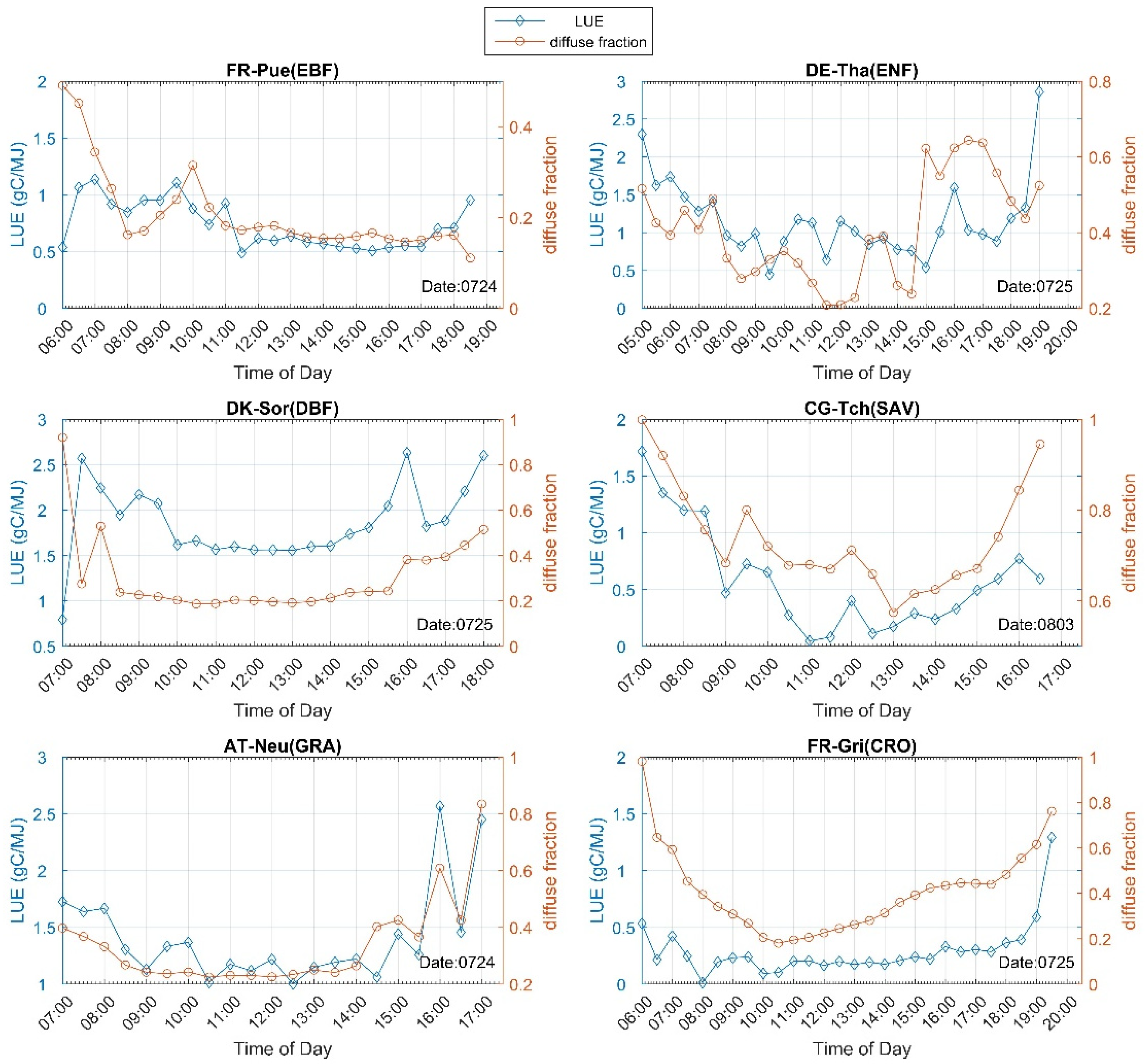
Daily variations of LUE and diffuse fraction were analyzed firstly to determine the relationship between LUE and diffuse radiation. Here, data from FLUXNET2015 and the EBR FAPAR product were used for deriving LUE values at a half-hourly scale. Data within the peak-growth seasons were selected for analysis. Figure 1 shows the variations of LUE and diffuse fraction at different times during a single day. Both LUE and diffuse fraction exhibited high values during sunrise and sunset times while lower values were observed around noontimes, which indicates a co-variation between LUE and diffuse fraction at a daily scale.
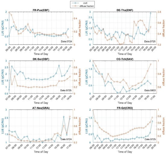
Figure 1.
Diurnal variations of LUE and diffuse fraction at FLUXNET sites.
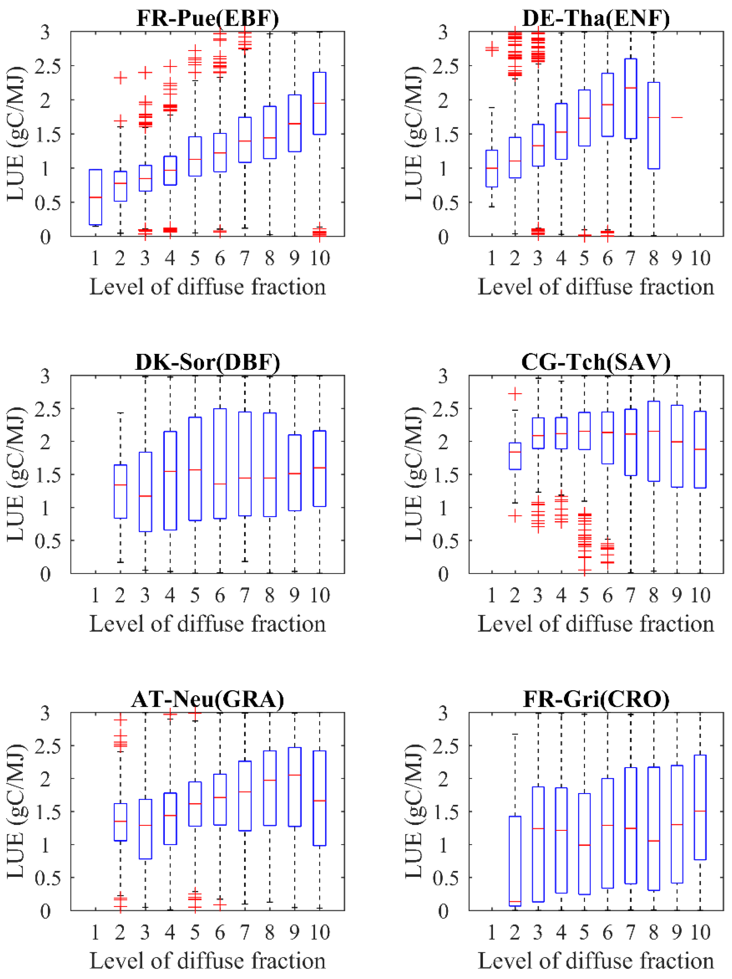
In addition, the relationship between LUE and diffuse fraction was examined across the FLUXNET sites within the whole year (Figure 2). For a better analysis, we firstly divided the diffuse fraction into ten levels from the lowest to the highest values (0.1 intervals). The results showed that LUE increased with increasing diffuse fraction for all vegetation types, which indicated the significant enhancement effect of diffuse radiation toward LUE [28,29].

Figure 2.
Temporal variations of LUE under different levels of diffuse radiation fraction at FLUXNET sites (The level of diffuse fraction denotes the values of diffuse fraction varying from 0 to 1 with 0.1 intervals).
3.2. Half-Hourly GPP Responses to Diffuse and Direct APAR at FLUXNET Sites
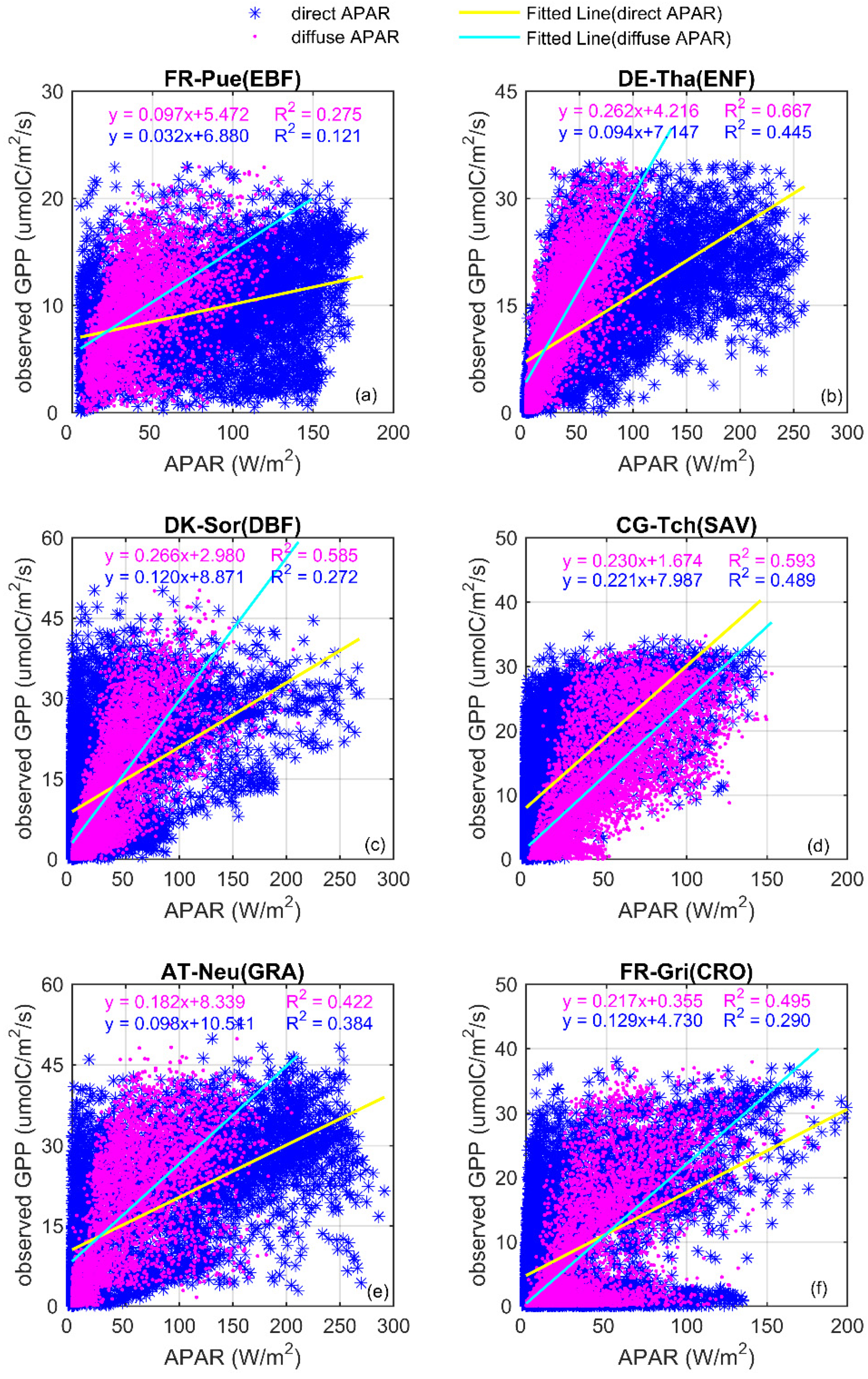
Figure 3 exhibits half-hourly FLUXNET GPP responses to diffuse and direct APAR at FLUXNET sites. The results in Figure 3 indicated a co-variation between GPP observations and APAR values under both diffuse and direct radiation conditions but with different rates, where GPP exhibited higher rates in diffuse radiation conditions. From the statistical results in Table 5, the slopes of the linear functions are extremely higher under diffuse radiation conditions (shown as magenta points, slopes varied from 0.097 to 0.266) than direct radiation conditions (shown as blue points, slopes varied from 0.032 to 0.221), which approximately three times the difference. Although the enhancement of R2 between the diffuse APAR and GPP than direct APAR was relatively small, obvious increase of slope values in the linear fitting functions (the variation coefficient of slope is up to 203.125% in the EBF site) can totally indicate a stronger response to GPP under diffuse radiation conditions. This was consistent with the results found by Zhou et al. [64]. Moreover, half-hourly GPP values were higher under diffuse light conditions than direct light conditions for the same amount of radiation, which further manifested the enhancement effect of LUE under diffuse radiation conditions [26,65].
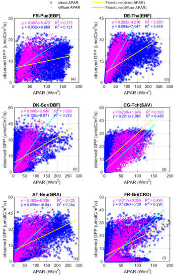
Figure 3.
GPP responses to diffuse and direct APAR at FLUXNET sites for different vegetation types: (a) EBF; (b) ENF; (c) DBF; (d) SAV; (e) GRA and (f) CRO. Observed GPP denotes half-hourly GPP derived from FLUXNET network.
Table 5.
The statistical metrics of the diffuse (left side) and direct APAR (right side) towards GPP.
3.3. Half-Hourly GPP Estimation by Diffuse and Direct APAR (DDA)-Based Method
In order to explore the effects of partitioning the diffuse and direct APAR on the half-hourly GPP estimation, site GPPs were collected from the FLUXNET2015 data sets. Meanwhile, the total APAR-based method was used as a comparison method. Figure 4 shows the validation of half-hourly GPP estimated by the diffuse and direct APAR-based model (GPP_DDA) and the total APAR-based GPP (GPP_TA) against the FLUXNET GPP (observed GPP) in six sites covering different vegetation types during the entire year. The results showed that GPP estimated using the DDA method presented higher R2 and lower RMSE values (R2 varied from 0.565 to 0.682, RMSE values were within the range of 3.219 to 12.405) against observed GPP than GPP_TA (R2 varied from 0.558 to 0.653, RMSE values ranged from 3.407 to 13.081), which indicated that the partition of diffuse and direct APAR in the GPP estimation can reduce the uncertainties when using big leaf models. In addition, a corrected RMSE value (see Section 2.7) was calculated for removing the scale difference between the satellite data and in-situ data as well as the systematic error of the big leaf-based model. Table 6 summarized the statistic metrics of DDA-based GPP and TA-based GPP with the observed GPP, concluding R2, RMSE, RMSE* and the variation coefficient of RMSE* values. From the result of the RMSE* values, obvious decrease of RMSE* values of the DDA-based GPP can be found in all vegetation types (the variation coefficient of RMSE* is varied between −11.224% and −23.015%). Moreover, a t test between these two models was used to indicate the difference between the DDA method and the total APAR-based method. The p-values were all less than 0.05 under a significance level of 0.05, which showed a significant difference in partitioning diffuse and direct APAR in the GPP estimation compared to the total APAR-based method.
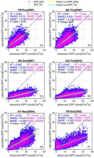
Figure 4.
Comparison of the calculated GPP and observed GPP for different vegetation types: (a) EBF; (b) ENF; (c) DBF; (d) SAV; (e) GRA, and (f) CRO (the label of “GPP_DDA” and “GPP_TA” denote the half-hourly GPP calculated using the DDA method and total APAR-based method; observed GPP are the half-hourly GPP derived from FLUXNET2015).
Table 6.
The statistic metrics of DDA-based GPP (left side) and TA-based GPP (right side) with observed GPP.
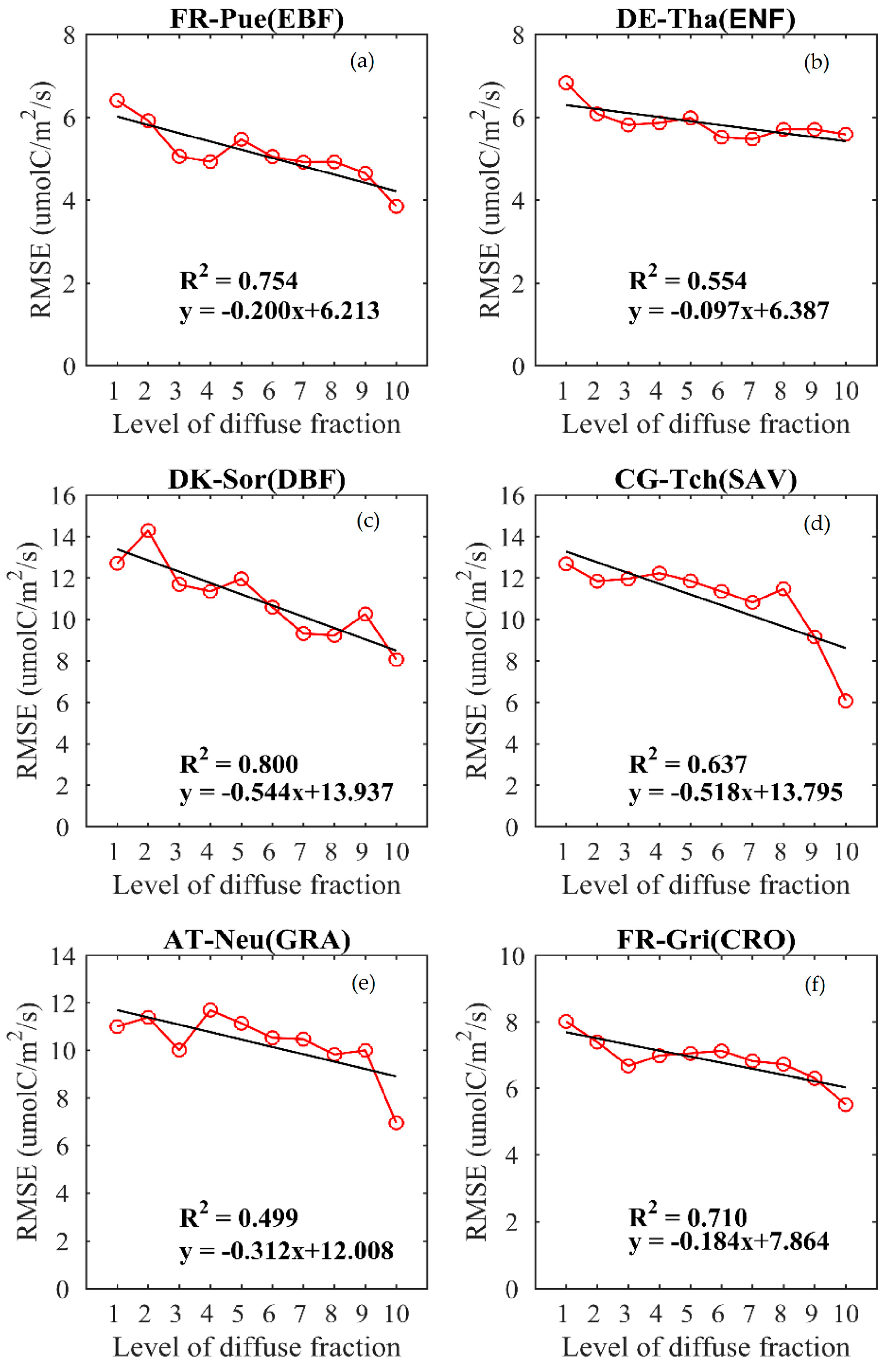
Besides, for a more intuitive validation of the DDA-based method, different levels of diffuse fraction are distinguished for calculating RMSE values between the DDA-based GPP and the observed GPP. Similarly to Figure 2, diffuse fraction was firstly divided in to ten groups, ranging from 0 to 1 with 0.1 intervals and the levels of diffuse fraction corresponds to 1 to 10 accordingly. Next, RMSE values between the DDA-based GPP and the observed GPP were calculated under different levels. Figure 5 shows the RMSE variation under different levels of diffuse fraction in different vegetation types over six FLUXNET sites. A significant decline of the RMSE values can be noticed with the increase of diffuse fraction owning averaged R2 values of 0.659, which indicated that the DDA-based method can well improve the accuracy of GPP estimation due to the influence of diffuse radiation and confirm the necessity of partitioning diffuse APAR on GPP estimations.
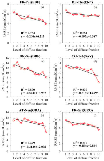
Figure 5.
RMSE variations between the DDA-based GPP and observed GPP under different levels of diffuse fraction in different vegetation types: (a) EBF; (b) ENF; (c) DBF; (d) SAV; (e) GRA, and (f) CRO (The level of diffuse fraction denotes the values of diffuse fraction varying from 0 to 1 with 0.1 intervals).
4. Discussion
4.1. Limitations of the Big Leaf Models
In Figure 4, higher R2 and lower RMSE values for the diffuse and direct APAR-based GPP compared to the FLUXNET GPP can be noticed, indicating that the partition of diffuse radiation in the GPP estimation is quite necessary. However, the enhancement of model performance was quite limited. The reason may be that the proposed diffuse and direct APAR-based (DDA) method was essentially a big leaf model, which treats the whole canopy as a big uniform leaf and does not separate the leaves into shaded and sunlit parts. Therefore, these simplifications may introduce systematic errors into the calculation of GPP [66,67,68]. Such big leaf model limitations might have significantly limited the effects of the partitioning by diffuse and direct APAR on the GPP estimation.
4.2. Uncertainties from LUE Simplifications
Due to of the lack of LUE observations under both direct and diffuse radiation conditions, LUE calculated from the EC-LUE model was assumed as LUE under clear-sky conditions, and obtained LUE values under diffuse radiation conditions afterwards multiplied the enhancement factor () [69]. This may certainly distort GPP estimations, but the point of this paper was to explore the effects of partitioning the direct and diffuse APAR in GPP estimations using big leaf models. Therefore, such simplification was reasonable here.
4.3. Scale Difference between Remote Sensing Data and In Situ Data
For model validation and comparison, FLUXNET GPP was used in this paper. From the scatter plots in Figure 4, scatters below the 1:1 line can be observed for DBF, SAV, GRA, and CRO sites, which indicates underestimations of both the direct and diffuse radiation (DDA) method and total APAR-based method. This may be a scale difference between the in situ data and remote sensing data. On the one hand, the in situ GPP data observed by FLUXNET was influenced by multiple factors, such as climate conditions (temperature, moisture, winds, etc.) and atmosphere conditions (clouds, aerosols, particles, etc.). On the other hand, the remote sensing data used in this paper included FAPAR and clumping index products, which represent the pixel information with a range of 500 m 500 m, while the in situ GPP data represent a single point. Furthermore, the vegetation types at FLUXNET sites were not actually totally homogenous, and the corresponding remote sensing pixels may not have represented the real value of the actual vegetation types. Therefore, the inconsistency in the in situ data and remote sensing data introduced uncertainties into model performance and validation results.
4.4. Uncertainties of the Remote Sensing Data
LAI, FAPAR, and CI satellite data were input to calculate the half-hourly FAPAR values across the FLUXNET sites in this paper. The quality of these inputs determined the accuracy of the GPP estimations. The MODIS LAI product (MCD15A2H), EBR FAPAR product, and CI product were used rather than measured data to drive the DDA model and the total APAR-based model. Such an application might have introduced uncertainties into the GPP estimations. In order to match the temporal scale of observations across the FLUXNET sites, a linear interpolation method was applied firstly for the EBR FAPAR product to obtain daily FAPAR and then to achieve half-hourly FAPAR records. Such an interpolation method might have introduced errors into the inputs of the GPP models. Additionally, LAI and CI data were used at temporal resolutions of eight days and a month, which might also have introduced errors into the GPP calculation at a half-hourly scale. In the future, high temporal and spatial resolution FAPAR, LAI and CI data should be used to constrain errors as well as for model construction and validation.
4.5. Contribution of Diffuse Radiation to GPP Estimations
The process of photosynthesis can be influenced by multiple environmental factors such as radiative conditions, vapor pressure deficit (VPD), and temperature [24,70]. The enhancement effect of LUE due to the diffuse radiation has been widely reported [24,28,29]. An approximate 110% enhancement of LUE under cloudy-sky days over clear-sky days was found by Choudhury [29]. Here, enhancement factors for different vegetation types derived from FLUXNET data by Zhang et al. [10] were used to correct LUE under diffuse radiation conditions.
Meanwhile, environmental factors such as VPD and major volcanic eruptions are also related to the diffuse radiation conditions [24,70]. Overall, the combined factors can enhance the photosynthesis under diffuse radiation conditions. Therefore, the partition of diffuse and direct radiation in GPP estimations is quite necessary.
5. Conclusions
In this paper, a diffuse and direct APAR-based (DDA) method is proposed to explore the effects of partitioning diffuse and direct APAR on half-hourly GPP estimations. The main conclusions are as follows:
- (1)
- LUE increased with increasing diffuse fraction for all vegetation types, which showed the enhancement effect of diffuse radiation on LUE. Moreover, a diurnal co-variation of LUE and diffuse fraction was observed for all vegetation types at FLUXNET sites, which further demonstrated the necessity of partitioning diffuse and direct APAR in half-hourly GPP estimations.
- (2)
- Half-hourly GPP increased with increasing diffuse and direct APAR but at different rates. Half-hourly GPP presented higher growth rates under diffuse conditions, with obvious increase of slope values (the variation coefficient of slope is up to 203.125%), which indicated the significant contribution of diffuse radiation to the process of vegetation photosynthesis.
- (3)
- Half-hourly GPP estimated using the DDA-based method showed higher R2, lower RMSE and RMSE* values (R2 varied from 0.565 to 0.682, RMSE ranged from 3.219 to 12.405 and RMSE* were within the range of 2.785 to 8.395) against the FLUXENET GPP than the GPP_TA (R2 varied from 0.558 to 0.653, RMSE ranged from 3.407 to 13.081 and RMSE* were within the range of 3.321 to 9.625), which suggested a better performance by partitioning the diffuse and direct APAR in half-hourly GPP estimations when using big leaf models.
Author Contributions
Conceptualization, S.C. and L.L.; methodology, S.C.; software, S.C.; validation, S.C. and X.L.; formal analysis, L.S.; investigation, S.C. and X.L.; resources, S.C. and L.L.; writing—original draft preparation, S.C.; writing—review and editing, S.C. and L.L.; supervision, L.L. and L.S.; funding acquisition, L.L. All authors have read and agreed to the published version of the manuscript.
Funding
This research was funded by the National Key Research and Development Program of China, grant number 2017YFA0603001 and National Natural Science Foundation of China, grant number 41825002.
Informed Consent Statement
Not applicable.
Acknowledgments
The authors gratefully acknowledge the CI products provided by Ziti Jiao at Beijing Normal University, the MODIS products obtained from the Land Products Land Processes Distributed Active Archive Center (LP DAAC), observations from FLUXNET2015 network and EC-LUE model proposed by Wenping Yuan at Sun Yat-sen University.
Conflicts of Interest
The authors declare no conflict of interest.
References
- Canadell, J.G.; Le Quéré, C.; Raupach, M.R.; Field, C.B.; Buitenhuis, E.T.; Ciais, P.; Conway, T.J.; Gillett, N.P.; Houghton, R.; Marland, G. Contributions to accelerating atmospheric CO2 growth from economic activity, carbon intensity, and efficiency of natural sinks. Proc. Natl. Acad. Sci. USA 2007, 104, 18866–18870. [Google Scholar] [CrossRef] [Green Version]
- Chen, J.M.; Mo, G.; Pisek, J.; Liu, J.; Deng, F.; Ishizawa, M.; Chan, D. Effects of foliage clumping on the estimation of global terrestrial gross primary productivity. Glob. Biogeochem. Cycles 2012, 26, 26. [Google Scholar] [CrossRef]
- Field, C.B.; Behrenfeld, M.J.; Randerson, J.T.; Falkowski, P. Primary production of the biosphere: Integrating terrestrial and oceanic components. Science 1998, 281, 237–240. [Google Scholar] [CrossRef] [Green Version]
- Field, C.B.; Barros, V.; Stocker, T.F.; Qin, D.; Dokken, D.J.; Ebi, K.L.; Midgley, P. Special Report of the Intergovernmental Panel on Climate Change; Intergovernmental Panel on Climate Change: Geneva, Switzerland, 2012. [Google Scholar]
- Potter, C.S.; Randerson, J.T.; Field, C.B.; Matson, P.A.; Vitousek, P.M.; Mooney, H.A.; Klooster, S.A. Terrestrial ecosystem production: A process model based on global satellite and surface data. Glob. Biogeochem. Cycles 1993, 7, 811–841. [Google Scholar] [CrossRef]
- Running, S.W.; Thornton, P.E.; Nemani, R.; Glassy, J.M. Global Terrestrial Gross and Net Primary Productivity from the Earth Observing System; Springer: New York, NY, USA, 2000. [Google Scholar]
- Xiao, X.; Hollinger, D.; Aber, J.; Goltz, M.; Davidson, E.A.; Zhang, Q.; Moore, B., III. Satellite-based modeling of gross primary production in an evergreen needleleaf forest. Remote Sens. Environ. 2004, 89, 519–534. [Google Scholar] [CrossRef]
- Xiao, X.; Zhang, Q.; Braswell, B.; Urbanski, S.; Boles, S.; Wofsy, S.; Moore, B., III; Ojima, D. Modeling gross primary production of temperate deciduous broadleaf forest using satellite images and climate data. Remote Sens. Environ. 2004, 91, 256–270. [Google Scholar] [CrossRef]
- Yuan, W.; Liu, S.; Zhou, G.; Zhou, G.; Tieszen, L.L.; Baldocchi, D.; Bernhofer, C.; Gholz, H.; Goldstein, A.H.; Goulden, M.L. Deriving a light use efficiency model from eddy covariance flux data for predicting daily gross primary production across biomes. Agric. For. Meteorol. 2007, 143, 189–207. [Google Scholar] [CrossRef] [Green Version]
- Zhang, Z.; Zhang, Y.; Zhang, Y.; Chen, J.M. Correcting clear-sky bias in gross primary production modeling from satellite solar-induced chlorophyll fluorescence data. J. Geophys. Res. Biogeosci. 2020, 125, e2020JG005822. [Google Scholar] [CrossRef]
- Baldocchi, D.; Falge, E.; Gu, L.; Olson, R.; Hollinger, D.; Running, S.; Anthoni, P.; Bernhofer, C.; Davis, K.; Evans, R. Fluxnet: A new tool to study the temporal and spatial variability of ecosystem-scale carbon dioxide, water vapor, and energy flux densities. Bull. Am. Meteorol. Soc. 2001, 82, 2415–2434. [Google Scholar] [CrossRef]
- Turner, D.P.; Ritts, W.D.; Cohen, W.B.; Gower, S.T.; Zhao, M.; Running, S.W.; Wofsy, S.C.; Urbanski, S.; Dunn, A.L.; Munger, J. Scaling gross primary production (gpp) over boreal and deciduous forest landscapes in support of modis gpp product validation. Remote Sens. Environ. 2003, 88, 256–270. [Google Scholar] [CrossRef] [Green Version]
- Zhao, M.; Heinsch, F.A.; Nemani, R.R.; Running, S.W. Improvements of the modis terrestrial gross and net primary production global data set. Remote Sens. Environ. 2005, 95, 164–176. [Google Scholar] [CrossRef]
- Zhao, M.; Running, S.W.; Nemani, R.R. Sensitivity of moderate resolution imaging spectroradiometer (modis) terrestrial primary production to the accuracy of meteorological reanalyses. J. Geophys. Res. Biogeosci. 2006, 111, G1. [Google Scholar] [CrossRef] [Green Version]
- Heinsch, F.A.; Zhao, M.; Running, S.W.; Kimball, J.S.; Nemani, R.R.; Davis, K.J.; Bolstad, P.V.; Cook, B.D.; Desai, A.R.; Ricciuto, D.M. Evaluation of remote sensing based terrestrial productivity from modis using regional tower eddy flux network observations. IEEE Trans. Geosci. Remote Sens. 2006, 44, 1908–1925. [Google Scholar] [CrossRef] [Green Version]
- Nightingale, J.; Coops, N.; Waring, R.; Hargrove, W. Comparison of modis gross primary production estimates for forests across the USA with those generated by a simple process model, 3-pgs. Remote Sens. Environ. 2007, 109, 500–509. [Google Scholar] [CrossRef] [Green Version]
- Wang, Y.; Woodcock, C.E.; Buermann, W.; Stenberg, P.; Voipio, P.; Smolander, H.; Häme, T.; Tian, Y.; Hu, J.; Knyazikhin, Y. Evaluation of the modis lai algorithm at a coniferous forest site in finland. Remote Sens. Environ. 2004, 91, 114–127. [Google Scholar] [CrossRef]
- Hill, M.J.; Senarath, U.; Lee, A.; Zeppel, M.; Nightingale, J.M.; Williams, R.D.J.; McVicar, T.R. Assessment of the modis lai product for australian ecosystems. Remote Sens. Environ. 2006, 101, 495–518. [Google Scholar] [CrossRef]
- Zhang, Y.; Yu, Q.; Jiang, J.; Tang, Y. Calibration of terra/modis gross primary production over an irrigated cropland on the North China plain and an alpine meadow on the tibetan plateau. Glob. Chang. Biol. 2008, 14, 757–767. [Google Scholar] [CrossRef]
- Running, S.W.; Nemani, R.R.; Heinsch, F.A.; Zhao, M.; Reeves, M.; Hashimoto, H. A continuous satellite-derived measure of global terrestrial primary production. Bioscience 2004, 54, 547–560. [Google Scholar] [CrossRef]
- Roderick, M.L.; Farquhar, G.D.; Berry, S.L.; Noble, I.R. On the direct effect of clouds and atmospheric particles on the productivity and structure of vegetation. Oecologia 2001, 129, 21–30. [Google Scholar] [CrossRef]
- Mercado, L.M.; Bellouin, N.; Sitch, S.; Boucher, O.; Huntingford, C.; Wild, M.; Cox, P.M. Impact of changes in diffuse radiation on the global land carbon sink. Nature 2009, 458, 1014–1017. [Google Scholar] [CrossRef] [Green Version]
- Oliphant, A.; Dragoni, D.; Deng, B.; Grimmond, C.; Schmid, H.-P.; Scott, S. The role of sky conditions on gross primary production in a mixed deciduous forest. Agric. For. Meteorol. 2011, 151, 781–791. [Google Scholar] [CrossRef]
- Zhang, M.; Yu, G.-R.; Zhuang, J.; Gentry, R.; Fu, Y.-L.; Sun, X.-M.; Zhang, L.-M.; Wen, X.-F.; Wang, Q.-F.; Han, S.-J. Effects of cloudiness change on net ecosystem exchange, light use efficiency, and water use efficiency in typical ecosystems of China. Agric. For. Meteorol. 2011, 151, 803–816. [Google Scholar] [CrossRef]
- Propastin, P.; Ibrom, A.; Knohl, A.; Erasmi, S. Effects of canopy photosynthesis saturation on the estimation of gross primary productivity from modis data in a tropical forest. Remote Sens. Environ. 2012, 121, 252–260. [Google Scholar] [CrossRef]
- Gu, L.; Baldocchi, D.; Verma, S.B.; Black, T.A.; Vesala, T.; Falge, E.M.; Dowty, P.R. Advantages of diffuse radiation for terrestrial ecosystem productivity. J. Geophys. Res. Atmos. 2002, 107, ACL 2. [Google Scholar] [CrossRef] [Green Version]
- Knohl, A.; Baldocchi, D.D. Effects of diffuse radiation on canopy gas exchange processes in a forest ecosystem. J. Geophys. Res. Biogeosci. 2015, 113, 143–144. [Google Scholar] [CrossRef]
- Alton, P.; North, P.; Los, S. The impact of diffuse sunlight on canopy light-use efficiency, gross photosynthetic product and net ecosystem exchange in three forest biomes. Glob. Chang. Biol. 2007, 13, 776–787. [Google Scholar] [CrossRef]
- Choudhury, B.J. Estimating gross photosynthesis using satellite and ancillary data: Approach and preliminary results. Remote Sens. Environ. 2001, 75, 1–21. [Google Scholar] [CrossRef]
- Agarwal, D.A.; Humphrey, M.; Beekwilder, N.F.; Jackson, K.R.; Goode, M.M.; van Ingen, C. A data-centered collaboration portal to support global carbon-flux analysis. Concurr. Comput. Pract. Exp. 2010, 22, 2323–2334. [Google Scholar] [CrossRef] [Green Version]
- Mccree, K.J. Test of current definitions of photosynthetically active radiation against leaf photosynthesis data. Agric. Meteorol. 1972, 10, 443–453. [Google Scholar] [CrossRef]
- Zheng, Y.; Shen, R.; Wang, Y.; Li, X.; Liu, S.; Liang, S.; Chen, J.M.; Ju, W.; Zhang, L.; Yuan, W. Improved estimate of global gross primary production for reproducing its long-term variation, 1982–2017. Earth Syst. Sci. Data 2020, 12, 2725–2746. [Google Scholar] [CrossRef]
- Monteith, J.L. Vegetation and the Atmosphere. Case Studies; Academic Press: Cambridge, MA, USA, 1976; Volume 2. [Google Scholar]
- Sellers, P.; Dickinson, R.; Randall, D.; Betts, A.; Hall, F.; Berry, J.; Collatz, G.; Denning, A.; Mooney, H.; Nobre, C. Modeling the exchanges of energy, water, and carbon between continents and the atmosphere. Science 1997, 275, 502–509. [Google Scholar] [CrossRef] [PubMed] [Green Version]
- Knyazikhin, Y.; Martonchik, J.V.; Myneni, R.B.; Diner, D.J.; Running, S.W. Synergistic algorithm for estimating vegetation canopy leaf area index and fraction of absorbed photosynthetically active radiation from modis and misr data. J. Geophys. Res. Atmos. 1998, 103, 32257–32275. [Google Scholar] [CrossRef] [Green Version]
- Gobron, N.; Pinty, B.; Aussedat, O.; Chen, J.M.; Cohen, W.B.; Fensholt, R.; Gond, V.; Huemmrich, K.F.; Lavergne, T.; Mélin, F. Evaluation of fraction of absorbed photosynthetically active radiation products for different canopy radiation transfer regimes: Methodology and results using joint research center products derived from seawifs against ground-based estimations. J. Geophys. Res. Atmos. 2006, 111, D13. [Google Scholar] [CrossRef]
- Gobron, N.; Pinty, B.; Verstraete, M.; Govaerts, Y. The meris global vegetation index (mgvi): Description and preliminary application. Int. J. Remote Sens. 1999, 20, 1917–1927. [Google Scholar] [CrossRef]
- Buchhorn, M.; Lesiv, M.; Tsendbazar, N.-E.; Herold, M.; Bertels, L.; Smets, B. Copernicus global land cover layers—Collection 2. Remote Sens. 2020, 12, 1044. [Google Scholar] [CrossRef] [Green Version]
- Liu, L.; Zhang, X.; Xie, S.; Liu, X.; Peng, D. Global white-sky and black-sky fapar retrieval using the energy balance residual method: Algorithm and validation. Remote Sens. 2019, 11, 1004. [Google Scholar] [CrossRef] [Green Version]
- Frederic, B.; Weiss, M.; Allard, D.; Garrigue, S.; Vintila, R. Valeri: A network of sites and methodology for the validation of medium spatial resolution land products. Remote Sens. Environ. 2005, 76, 36–39. [Google Scholar]
- Myneni, R.; Knyazikhin, Y.; Park, T. Mcd15a2h Modis/Terra+ Aqua Leaf Area Index/fpar 8-Day l4 Global 500 m sin Grid v006 [Data Set]. 2015. Available online: https://data.tpdc.ac.cn/zh-hans/data/literature/682841a1-f889-4e63-aac3-2991097d00df/ (accessed on 19 December 2021).
- Myneni, R.B.; Hoffman, S.; Knyazikhin, Y.; Privette, J.; Glassy, J.; Tian, Y.; Wang, Y.; Song, X.; Zhang, Y.; Smith, G. Global products of vegetation leaf area and fraction absorbed par from year one of modis data. Remote Sens. Environ. 2002, 83, 214–231. [Google Scholar] [CrossRef] [Green Version]
- Chen, J.M.; Menges, C.H.; Leblanc, S.G. Global mapping of foliage clumping index using multi-angular satellite data. Remote Sens. Environ. 2005, 97, 447–457. [Google Scholar] [CrossRef]
- Jiao, Z.; Dong, Y.; Schaaf, C.B.; Chen, J.M.; Román, M.; Wang, Z.; Zhang, H.; Ding, A.; Erb, A.; Hill, M.J. An algorithm for the retrieval of the clumping index (ci) from the modis brdf product using an adjusted version of the kernel-driven brdf model. Remote Sens. Environ. 2018, 209, 594–611. [Google Scholar] [CrossRef]
- Farquhar, G.D.; von Caemmerer, S.V.; Berry, J.A. A biochemical model of photosynthetic CO2 assimilation in leaves of c 3 species. Planta 1980, 149, 78–90. [Google Scholar] [CrossRef] [PubMed] [Green Version]
- Collatz, G.J. Physiological and environmental regulation of stomatal conductance, photosynthesis and transpiration: A model that includes a laminar boundary layer. Agri. For. Met. 1991, 54, 107–136. [Google Scholar] [CrossRef]
- Prentice, I.C.; Dong, N.; Gleason, S.M.; Maire, V.; Wright, I.J. Balancing the costs of carbon gain and water transport: Testing a new theoretical framework for plant functional ecology. Ecol. Lett. 2014, 17, 82–91. [Google Scholar] [CrossRef] [PubMed]
- Keenan, T.F.; Prentice, I.C.; Canadell, J.G.; Williams, C.A.; Wang, H.; Raupach, M.; Collatz, G.J. Recent pause in the growth rate of atmospheric co 2 due to enhanced terrestrial carbon uptake. Nat. Commun. 2016, 7, 1–10. [Google Scholar] [CrossRef] [Green Version]
- Korson, L.; Drost-Hansen, W.; Millero, F.J. Viscosity of water at various temperatures. J. Phys. Chem. 1969, 73, 34–39. [Google Scholar] [CrossRef]
- Raich, J.; Rastetter, E.; Melillo, J.M.; Kicklighter, D.W.; Steudler, P.; Peterson, B.; Grace, A.; Moore, B., III; Vorosmarty, C.J. Potential net primary productivity in south america: Application of a global model. Ecol. Appl. 1991, 1, 399–429. [Google Scholar] [CrossRef] [PubMed] [Green Version]
- Yuan, W.; Zheng, Y.; Piao, S.; Ciais, P.; Lombardozzi, D.; Wang, Y.; Ryu, Y.; Chen, G.; Dong, W.; Hu, Z. Increased atmospheric vapor pressure deficit reduces global vegetation growth. Sci. Adv. 2019, 5, eaax1396. [Google Scholar] [CrossRef] [Green Version]
- Monteith, J. Solar radiation and productivity in tropical ecosystems. J. Appl. Ecol. 1972, 9, 747–766. [Google Scholar] [CrossRef] [Green Version]
- Yuan, W.; Liu, S.; Yu, G.; Bonnefond, J.-M.; Chen, J.; Davis, K.; Desai, A.R.; Goldstein, A.H.; Gianelle, D.; Rossi, F. Global estimates of evapotranspiration and gross primary production based on modis and global meteorology data. Remote Sens. Environ. 2010, 114, 1416–1431. [Google Scholar] [CrossRef] [Green Version]
- Chen, J.M. Canopy architecture and remote sensing of the fraction of photosynthetically active radiation absorbed by boreal conifer forests. IEEE Trans. Geosci. Remote Sens. 1996, 34, 1353–1368. [Google Scholar] [CrossRef]
- Nilson, T. A theoretical analysis of the frequency of gaps in plant stands. Agric. Meteorol. 1971, 8, 25–38. [Google Scholar] [CrossRef]
- Nilson, T. Inversion of gap frequency data in forest stands. Agric. For. Meteorol. 1999, 98, 437–448. [Google Scholar] [CrossRef]
- Majasalmi, T.; Bright, R.M. Evaluation of leaf-level optical properties employed in land surface models-example with CLM 5.0. Geosci. Model Dev. 2019, 12, 3923–3938. [Google Scholar] [CrossRef] [Green Version]
- Goel, N.S.; Thompson, R.L. Inversion of vegetation canopy reflectance models for estimating agronomic variables. V. Estimation of leaf area index and average leaf angle using measured canopy reflectances. Remote Sens. Environ. 1984, 16, 69–85. [Google Scholar] [CrossRef]
- Wilson, J.W. Inclined point quadrats. New Phytol. 1960, 59, 1–7. [Google Scholar] [CrossRef]
- Wilson, J.W. Stand structure and light penetration. III. Sunlit foliage area. J. Appl. Ecol. 1967, 4, 159. [Google Scholar] [CrossRef]
- Jacquemoud, S.; Baret, F. Prospect: A model of leaf optical properties spectra. Remote Sens. Environ. 1990, 34, 75–91. [Google Scholar] [CrossRef]
- Hosgood, B.; Jacquemoud, S.; Andreoli, G.; Verdebout, J.; Pedrini, G.; Schmuck, G. Leaf optical properties experiment 93. Jt. Res. Cent. Eur. Comm. Inst. Remote Sens. ApJacquemoud 1995, 75–91. Available online: https://data.ecosis.org/dataset/13aef0ce-dd6f-4b35-91d9-28932e506c41/resource/4029b5d3-2b84-46e3-8fd8-c801d86cf6f1/download/leaf-optical-properties-experiment-93-lopex93.pdf (accessed on 19 December 2021).
- Feret, J.-B.; François, C.; Asner, G.P.; Gitelson, A.A.; Martin, R.E.; Bidel, L.P.; Ustin, S.L.; Le Maire, G.; Jacquemoud, S. Prospect-4 and 5: Advances in the leaf optical properties model separating photosynthetic pigments. Remote Sens. Environ. 2008, 112, 3030–3043. [Google Scholar] [CrossRef]
- Zhou, H.; Yue, X.; Lei, Y.; Zhang, T.; Cao, Y. Responses of gross primary productivity to diffuse radiation at global fluxnet sites. Atmos. Environ. 2021, 244, 117905. [Google Scholar] [CrossRef]
- Yue, X.; Unger, N. Fire air pollution reduces global terrestrial productivity. Nat. Commun. 2018, 9, 1–9. [Google Scholar] [CrossRef]
- De Pury, D.; Farquhar, G. Simple scaling of photosynthesis from leaves to canopies without the errors of big-leaf models. Plant Cell Environ. 1997, 20, 537–557. [Google Scholar] [CrossRef]
- Wang, Y.-P.; Leuning, R. A two-leaf model for canopy conductance, photosynthesis and partitioning of available energy I: Model description and comparison with a multi-layered model. Agric. For. Meteorol. 1998, 91, 89–111. [Google Scholar] [CrossRef]
- Chen, J.; Liu, J.; Cihlar, J.; Goulden, M. Daily canopy photosynthesis model through temporal and spatial scaling for remote sensing applications. Ecol. Model. 1999, 124, 99–119. [Google Scholar] [CrossRef] [Green Version]
- Urban, O.; Janouš, D.; Acosta, M.; Czerný, R.; Markova, I.; Navratil, M.; Pavelka, M.; Pokorný, R.; Šprtová, M.; Zhang, R. Ecophysiological controls over the net ecosystem exchange of mountain spruce stand. Comparison of the response in direct vs. diffuse solar radiation. Glob. Chang. Biol. 2007, 13, 157–168. [Google Scholar] [CrossRef]
- Proctor, J.; Hsiang, S.; Burney, J.; Burke, M.; Schlenker, W. Estimating global agricultural effects of geoengineering using volcanic eruptions. Nature 2018, 560, 480–483. [Google Scholar] [CrossRef]

Publisher’s Note: MDPI stays neutral with regard to jurisdictional claims in published maps and institutional affiliations. |
© 2021 by the authors. Licensee MDPI, Basel, Switzerland. This article is an open access article distributed under the terms and conditions of the Creative Commons Attribution (CC BY) license (https://creativecommons.org/licenses/by/4.0/).