Abstract
Salinity is the primary determinant of the Arctic Ocean’s density structure. Freshwater accumulation and distribution in the Arctic Ocean have varied significantly in recent decades and certainly in the Beaufort Gyre (BG). In this study, we analyze salinity variations in the BG region between 2012 and 2017. We use in situ salinity observations from the Seasonal Ice Zone Reconnaissance Surveys (SIZRS), CTD casts from the Beaufort Gyre Exploration Project (BGP), and the EN4 data to validate and compare with satellite observations from Soil Moisture Active Passive (SMAP), Soil Moisture and Ocean Salinity (SMOS), and Aquarius Optimally Interpolated Sea Surface Salinity (OISSS), and Arctic Ocean models: ECCO, MIZMAS, HYCOM, ORAS5, and GLORYS12. Overall, satellite observations are restricted to ice-free regions in the BG area, and models tend to overestimate sea surface salinity (SSS). Freshwater Content (FWC), an important component of the BG, is computed for EN4 and most models. ORAS5 provides the strongest positive SSS correlation coefficient (0.612) and lowest bias to in situ observations compared to the other products. ORAS5 subsurface salinity and FWC compare well with the EN4 data. Discrepancies between models and SIZRS data are highest in GLORYS12 and ECCO. These comparisons identify dissimilarities between salinity products and extend challenges to observations applicable to other areas of the Arctic Ocean.
1. Introduction
Arctic Ocean salinity is a key element of seasonal and interannual variability [1]. In this paper, we provide a comparison regarding modeled, remotely sensed, and directly observed salinity in the Arctic Ocean. We had two objectives. First, we wished to learn the validity of remotely sensed and modeled salinity compared to in situ observations. Low water temperatures and the consequently low thermal expansion coefficient make Arctic Ocean salinity the primary determinant of stratification and the density distribution controlling geostrophic circulation. This, combined with the facts that surface buoyancy fluxes resulting from sea ice formation and melt are due overwhelmingly to salt flux, and that the inflows to the Arctic Ocean are characterized by large differences in salinity, results in the Arctic Ocean being a salt-stratified sea. Furthermore, the Arctic Ocean is a critical link in the global freshwater–thermohaline chain, where the high salinity Atlantic Water combines with less saline Pacific Water and runoff from drainage basins extends south beyond the Arctic Circle. While salinity is important, owing to the ice cover and remoteness, it is extremely difficult to make in situ observations of salinity in critical areas of the Arctic Ocean. Ultimately, we must rely on remote sensing and models to infer salinity changes in these areas.
Second, we sought a better understanding of Arctic Ocean salinity and freshwater content (FWC) changes, with special emphasis on the Beaufort Sea. The mean density structure and wind-driven surface circulation of the Arctic Ocean are largely dominated by the anticyclonic Beaufort Gyre in the Canadian Basin, along with the Transpolar Drift from the Pacific side of the Arctic Basin, over the Pole to the Fram Strait gateway to the North Atlantic. Consequently, changes in the Beaufort Gyre circulation and freshwater storage have been studied extensively in recent decades [2,3,4]) and are of current interest in their own right.
However, analysis of changes relative to the time-averaged Arctic Ocean circulation and freshwater distribution over the last 70 years reveal that the leading pattern of variability is centered not in the Beaufort Sea, but on the Russian side of the Arctic Ocean. In its positive phase, this pattern is dominated by a sea surface trough with cyclonic circulation roughly around in the Makarov Basin [5]. The positive (or Cyclonic Mode) phase became more dominant, along with an increase in area-average Arctic Ocean vorticity, beginning in 1990 and associated with a one standard deviation increase in the average winter Arctic Oscillation index. As part of this regime shift, the dominant mode tends to include an increase in the intensity, but not the size, of the anticyclonic Beaufort Gyre adjacent to the dominant growing and intensifying cyclonic circulation centered on the Makarov Basin.
As a consequence of these findings, we need to see increased observations on the Russian margins of the Arctic Basin. Without them, we are blind to the dominant mode of variability in circulation and freshwater pathways [6]. The extreme remoteness of this region has resulted in there being virtually no modern repeat in situ observations there. Therefore, we looked to this study to not only explore salinity in the observation-rich Beaufort Sea for its own sake but to validate modeled salinities and remotely sensed sea surface salinity (SSS) with which to infer salinity on the observation-poor Russian side of the Arctic Ocean in future studies.
This paper is structured as follows. Section 2 will detail the data used from each product: satellite observations, ocean model simulations, and in situ measurements. Section 3 provides research results followed by a related discussion in Section 4. Section 5 will summarize our conclusions of this study.
2. Observations and Models
We used a multiple-product analysis to evaluate salinity comparisons between in situ observations, satellite missions, and ocean models. Our study covers January 2012 to December 2017, and matches the availability of all salinity products used in this study. There are inherent differences between products on temporal and spatial scales. While satellites can only observe the top few centimeters of the ocean, measurements from profiling instruments stabilize between a depth of 2 m, and ocean models typically start estimations at a 5 m depth. Vertical layers varied between ocean models and were therefore linearly interpolated to the depths of in situ observations.
The liquid FWC calculation quantifies the vertically integrated salinity anomaly from a particular reference salinity (Sref), which in this case is 34.8 psu indicated by the mean of the Arctic Ocean and commonly used in other studies [7,8,9]. Following Carmack et al. [10], Fuentes-Franco et al. [11], and Dewey et al. [12], we calculate integrated liquid FWC (m) from salinity measurements and estimations using the equation:
where S(z) indicates the salinity (psu) versus depth z. We integrate FWC from 5 m, based on the initial depth available from all models, to 500 m depth to encompass the important components of the upper Arctic Ocean.
2.1. Observations
2.1.1. Satellite Data
We use three sensor products that rely on passive microwave radiometry to observe oceanic parameters on the sea surface. The Soil Moisture and Ocean Salinity (SMOS) Version 3.1 SSS product produced at the Barcelona Expert Center (BEC) is especially useful in that it was specifically designed to measure ocean surface salinity in the Arctic region. The product has a spatial resolution of 25 km and uses an Equal-Area Scalable Earth (EASE)–Grid 2.0 with a temporal resolution of 3 days spanning from 2011–2019. A later mission, the Soil Moisture Active Passive (SMAP), has provided data since 2015 and is available via the Physical Oceanography Distributed Active Archive (PO.DAAC). This 0.25° × 0.25° gridded product is based on the latest version 4.0 data from Remote Sensing Systems (RSS) Level 3 SSS, including 8-day running means [13,14]. The latest version includes higher coastal resolutions and a sea-ice mask algorithm reliant on RSS AMSR–2–sea–maps. The third satellite-based product used in this research is the Multi-Mission Optimally Interpolated Sea Surface Salinity (OISSS) Level 4 V1.0 [15]. This dataset was produced by the International Pacific Research Center (IPRC), University of Hawaii at Manoa, in association with RSS, Santa Rosa, California. Data combines SMOS, SMAP, and Aquarius/SAC-D mission observations on a 0.25° × 0.25° spatial grid with a 4-day temporal resolution using optimal interpolation and is available on the PO.DAAC data portal from 28 August 2011 to present [16,17].
2.1.2. In Situ Measurements
The Office of Naval Research sponsored Seasonal Ice Zone Reconnaissance Surveys (SIZRS) have been conducted since 2012 by the University of Washington Polar Science Center onboard US Coast Guard C–130 aircraft to create ocean and atmosphere sections across the Beaufort Sea seasonal ice zone (SIZ) [6]. The sections are created once a month during the summer melt season, typically June—October. Ocean stations are located at each degree of latitude along the 150°W longitude line from 72°N to 76°N or beyond the ice edge, whichever is farther north. Conductivity–Temperature–Depth (CTD) and current profiles are made using Sippican/Tsurumi–Seiki (TSK) Aircraft eXpendable CTDs (AXCTD) and Sippican Aircraft eXpendable Current Profilers (AXCP) that are dropped in open water or through leads in the sea ice and transmit profile data in real time to the aircraft’s antenna for recording onboard.
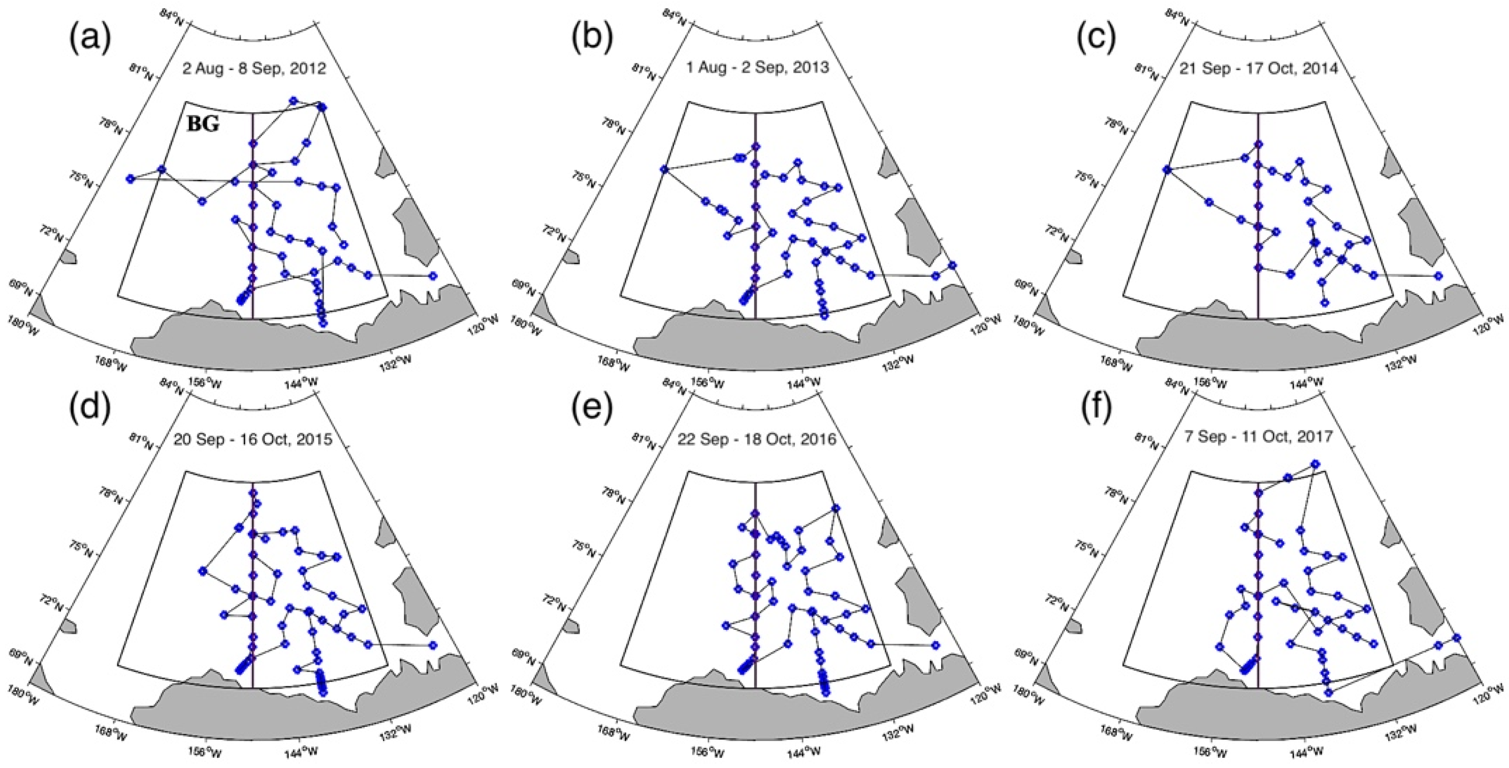
The Beaufort Gyre Exploration Project (BGP) is based at the WHOI in collaboration with researchers from Fisheries and Oceans Canada at the Institute of Ocean Sciences. Data have been collected using buoys and moorings since 2003. For this study, we use hydrographic profiles collected by annual CTD surveys in the BG region (Figure 1). Locations of the CTD casts were not uniform in the BG boundary but were consistently taken along the 150°W longitude (purple line), which we use for transect average comparisons.
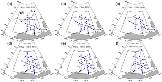
Figure 1.
Map of the Beaufort Gyre Exploration Project (BGP) CTD casts (blue dots) from (a–f) 2012–2017 in the (black outline) Beaufort Gyre (BG). The line along 150°W delineates the transect between 70.5°N and 80.5°N.
The Met Office Hadley Center “EN” series global objective analysis product’s most recent version 4.2.1 (EN4) provides monthly ocean temperature and salinity profiles with objective analyses and uncertainty estimates since 1900 [18]. EN4 salinity data relies on observations from Argo floats, Arctic Synoptic Basinwide Oceanography, Global temperature and salinity profile program, and the world ocean database. Salinity profiles are available on uniform 1° horizontal resolutions with 42 depth levels beginning at a 5-m depth.
2.2. Ocean Model Simulations and Reanalysis Products
We used numerous ocean model simulations and reanalysis products to compare among their different base models, spatiotemporal resolutions, and assimilation methods, of which summaries are provided in Table 1.

Table 1.
Summary of ocean model characteristics used in this study.
The first model used in this study was the National Aeronautics and Space Administration’s (NASA) Estimating the Circulation and Climate of the Ocean (ECCO): version 4, release 4 (v4r4) modeling system [19,20]. ECCOv4r4 uses a Lat–Lon–Cap 90 (LLC90) grid with varying horizontal resolutions between 110-km at mid-latitudes and 22-km in polar regions. ECCOv4r4 provided daily salinity data from January 1992 to December 2017 [21].
The Marginal Ice Zone Modeling and Assimilation System (MIZMAS) developed by the Applied Physics Laboratory Polar Science Center (APL/PSC) produces 3–D daily salinity estimates starting at a 2.5-m depth and horizontal resolutions to about 20 km [22]. Reanalysis data from NCEP/NCAR is incorporated into the atmospheric forcing, to drive the seven ensemble predictions [23,24]. Further information regarding the MIZMAS ice-ocean model is detailed by Zhang et al. [25] in conjunction with other product analyses. We obtained MIZMAS data from PSC for 2012–2017 for the Pacific Arctic Ocean region.
The Hybrid Coordinate Ocean Model (HYCOM) sponsored by the National Ocean Partnership Program (NOPP) is coupled with the Los Alamos Sea Ice model (CICE), which provides SSS simulations at a 1/12° global spatial resolution [26,27]. Daily data is processed by averaging 12-h data and computes real-time simulations and forecast verification statistics of oceanic, sea ice, and atmospheric conditions. Atmospheric forcing is provided by the Fleet Numerical Meteorology and Oceanography Center 3-hrly 0.281° Navy Global Environmental Model.
We use monthly salinity data provided by the European Centre for Medium-Range Weather Forecasts (ECMWF) through the Ocean Reanalysis System’s version 5 (ORAS5), which uses the Nucleus for European Modeling of the Ocean (NEMOv3.4) for its ocean model coupled with a sea ice model [28]. This version consists of eddy-permitting 1/4° horizontal resolution with 75 vertically stratified layers and is available via the Integrated Climate Data Center (ICDC) at the University of Hamburg. ORAS5 derived its forcing fields from ERA–Interim, an atmospheric reanalysis, until 2015 [29]. The post–2015 reanalysis product uses revised CORE bulk formulas and wave forcing from the ECMWF Numerical Weather Prediction (NWP) model [30,31].
GLORYS12 Version 1 is a global ocean eddy-resolving reanalysis product produced by Mercator Ocean International and based on the Copernicus Marine Service (CMEMS) forecasting system. Like ORAS5, the model constituent of GLORYS12 uses the NEMO platform driven at the surface by ECMWF ERA–Interim atmospheric reanalysis. Salinity data was provided daily from 1993–2019 at a 1/12° spatial resolution with 50 standard vertical layers starting at 0.5 m [32].
3. Results
3.1. Sea Surface Salinity
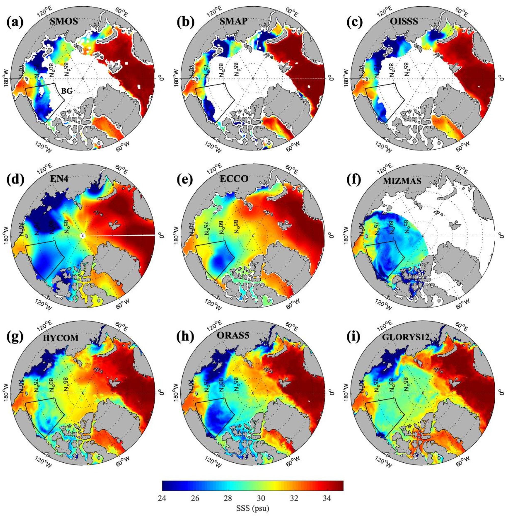
The Arctic Ocean serves as a connection between the less saline North Pacific Ocean and the more saline North Atlantic Ocean, and these contrasting salinity characteristics determine the dominant structure of the Arctic Ocean FWC. To examine all products, including the open–water surface restricted remote sensing observations, we first assessed SSS averaged over September 2015 (Figure 2), the month when minimum sea ice extent typically occurs [33]. The BG region, as an area of interest for this study, was outlined in a black box. Overall, the salinity values between observations and estimations agree on large spatial scales. For example, high salinities are prominent on the North Atlantic side of the Arctic Ocean extending from the Nordic Sea, compared to the lower salinities on the North Pacific side owing to the relatively fresh inflow of Pacific Water through the Bering Strait. Fresher waters observed over the Russian continental shelf are near the discharge regions of major Russian rivers, i.e., the Ob, Yenisey, and Lena rivers. However, the local salinity details can be quite different among the products. In particular, local salinity variances between models are apparent in the western part of the Kara Sea, the Canadian Archipelago, the coastal edges of Greenland, and notably in the BG.
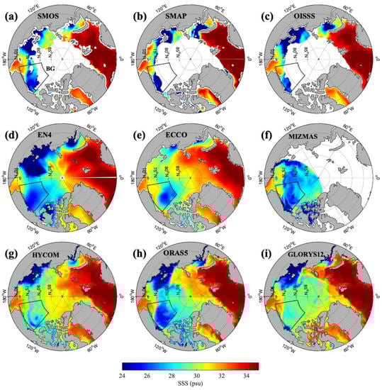
Figure 2.
Arctic Ocean sea surface salinity (SSS) averaged over the month of September 2015 from satellites: (a) SMOS, (b) SMAP, (c) OISSS, objective analysis product: (d) EN4, and ocean model simulations: (e) ECCO, (f) MIZMAS, (g) HYCOM, (h) ORAS5, and (i) GLORYS12.
While all satellite SSS measurements are restricted to the open-water regions between the coast and ice edge, SMOS provides higher coverage of data in the Arctic Ocean compared to SMAP or OISSS, especially in the Amerasian Basin (Figure 2a–c). The EN4 data and models resolve salinities close to Arctic Ocean coastlines, and with the exception of ECCO and MIZMAS, extend even into the Ob River channel. MIZMAS data provided is tuned for and restricted to the Canadian Basin. Low salinity in MIZMAS extends throughout the BG region and across the northern Chukchi Sea to the East Siberian Sea, which is not as pronounced in other products. The lower salinity observed in MIZMAS can potentially be attributed to calibration with SIZ hydrographic data and incorporation of floe size distributions in the model. EN4 has the largest horizontal resolution gridded at 1 degree. Therefore, the interpolation of SSS is not as refined as the salinity in the ocean models. Modeling constituents are similar between ORAS5 and GLORYS12 reanalysis products, but GLORYS12 illustrates more saline waters than ORAS5 near the pole, in the Canadian Archipelago, and in the Canadian Basin.
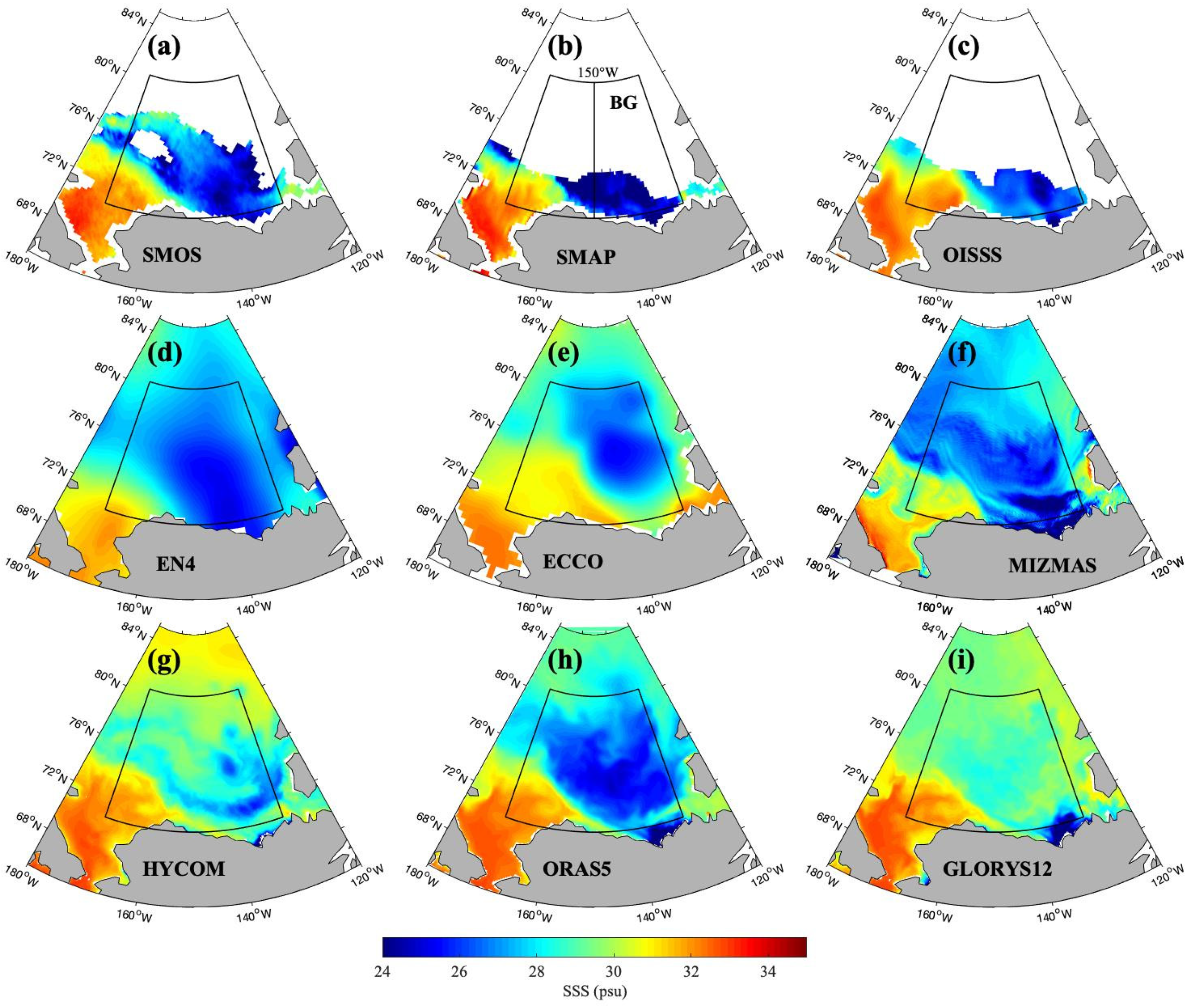
SSS in the BG Region is further emphasized in Figure 3, which provides evidence of distinctive regional salinity differences between the products. Overall, the products show relatively lower salinity in the central and eastern portions of the outlined BG region and more saline waters near the southwest portion, where the North Pacific inflow is near the surface. Satellite observations are especially limited in the northeast BG region (Figure 2a–c). HYCOM and MIZMAS illustrate band-type patterns of alternating lower and higher salinity values between latitudes, in contrast to other products that show gradual freshening towards the center of the BG. Compared with other models, MIZMAS has the lowest salinity at the mouth of the Mackenzie River and along the Alaskan coast. Interpolation of EN4 produces a more homogeneous appearance of lower salinity throughout the BG area. As with EN4, ORAS5 contains a large span of low salinity in the BG, but with more variations at smaller spatial scales. The GLORYS12 product had the highest salinity in September 2015 throughout the BG region.
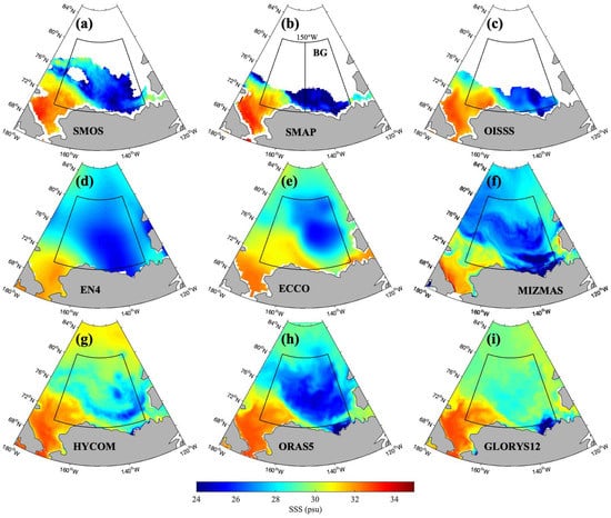
Figure 3.
Arctic Ocean sea surface salinity (SSS) averaged over the month of September 2015 in the Beaufort Gyre (BG) region derived from satellites: (a) SMOS, (b) SMAP, (c) OISSS, objective analysis product: (d) EN4, and ocean model simulations: (e) ECCO, (f) MIZMAS, (g) HYCOM, (h) ORAS5 and (i) GLORYS12. 150°W transect is outlined for comparisons in this study.
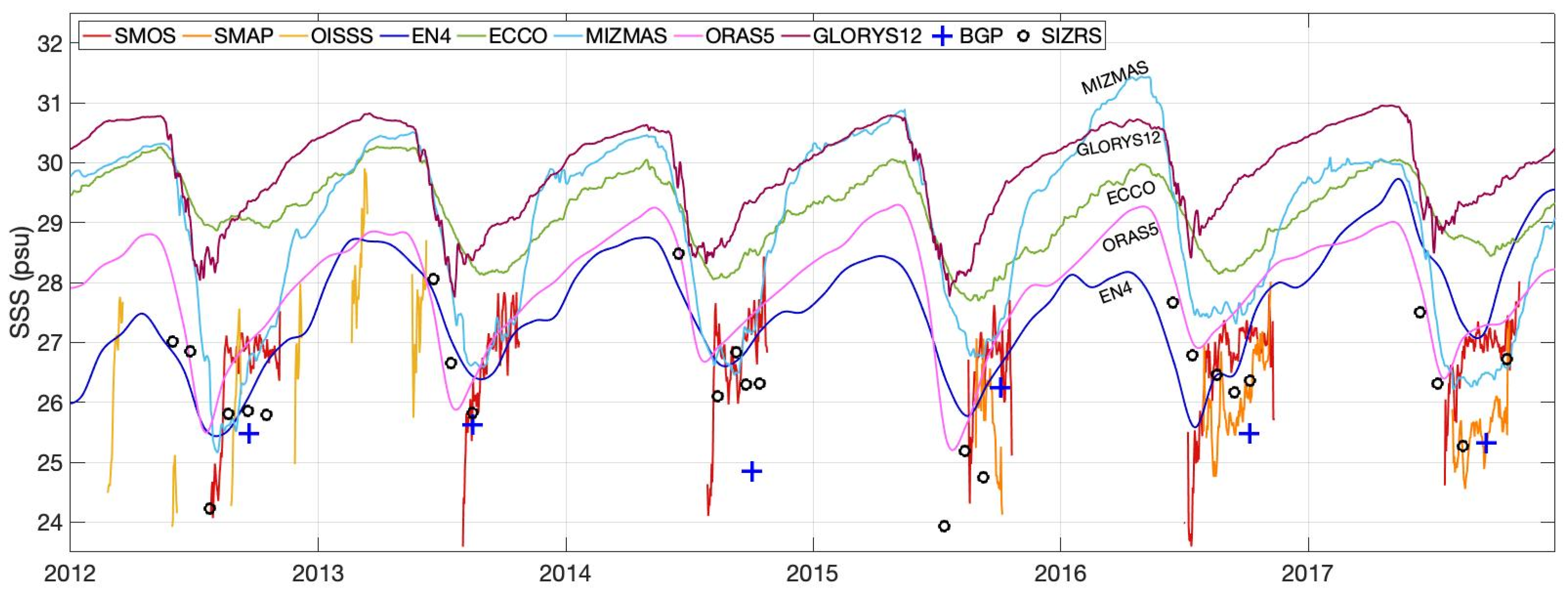
SIZRS and BGP have examined salinity and freshwater conditions in the BG using a multitude of in situ techniques, with the most persistent repeat sections conducted along 150°W longitude. Therefore, to further compare the salinity in the BG, we refined our analysis to a transect average at the BG region’s center longitude (150°W, 70.5°N–80.5°N) (Figure 4). Transect averages of SIZRS salinity show consistent annual patterns in which peaks occur around May and decrease to a minimum during July or August. SIZRS contains a few points that are much lower than in other years, such as July of 2012 and 2015. In Figure 4, SSS provided by BGP CTD casts denote the average date that data were collected along the transect during each annual expedition. BGP closely matched SIZRS, with the exception of 2014 and 2015, where differences were greater than 1, perhaps due to differences in the timing of the transects. Satellite-derived salinities below 15 psu were excluded due to possible sea ice contamination that could confuse product comparisons. Satellites showed the most drastic variations in salinity, likely due to variation of data coverage along 150°W. In general, SMOS and SMAP related to averaged SSS of the in situ and EN4 product, with most values within 1 psu while OISSS was more variable on shorter timescales.
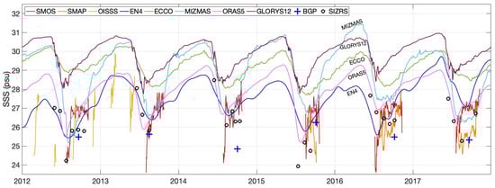
Figure 4.
Averaged sea surface salinity (SSS) along a 150°W transect between 70.5°N–80.5°N as seen in Figure 1 among ocean products between January 2012–December 2017.
Transect averages of SSS from the ocean models were comparable to the EN4 data in the sense that peaks occur before summer, around April, and the SSS minimum occurs abruptly towards July (Figure 4). However, the average differences of the model SSS from EN4 ranged between 0.35 psu (ORAS) to 2.3 psu (GLORYS12). The EN4 data shows its minimum (maximum) SSS during autumn (spring), reaching its largest magnitude at 25.5 psu (29.71 psu). MIZMAS showed a wide range of seasonal SSS fluctuations, with its lowest salinity in autumn 2012 around 25.2 psu and highest salinity near 31.45 psu in 2016. MIZMAS salinity values were comparable to GLORYS12 during winter months, then abruptly decreased by summer, closer to in situ and satellite products. ECCO estimated intermediate ranges between 27.84 psu and 30.28 psu throughout the time range. GLORYS12 and ORAS5 showed earlier minimum SSS dates in September at 31 psu and 29.3 psu, respectively, whereas other models reached a minimum shortly after October. GLORYS12 reached consistently high SSS maximums near 31 psu.
The in situ data from BGP and SIZRS were not continuous. Therefore, we matched the products to the specific times and latitude of 126 SIZRS AXCTD, drops made between 2012 and 2017 along the 150°W transect. We collocated remote sensing and model estimates of SSS to the date and latitude of each AXCTD drop. SIZRS measurements began at shallow depths but showed near-surface transients. Consequently, we compared SIZRS measurements at 2 m depth to satellites that measure salinity within the top few centimeters of the surface. The shallowest depth layer of many models begins at 5 m and therefore was compared to SIZRS at 5m. Product observations and estimates were available at each of the 126 SIZRS drops except for SMOS, SMAP, and BGP, which had 61, 27, and 32 samples at near-matching locations and times.
Figure 5 shows SSS comparisons between SIZRS and other products at each SIZRS drop (Figure 5). SIZRS salinity, at both a 2-m and 5-m, ranged from 23 psu to just below 31 psu. Satellites show a larger range of salinity compared to that of SIZRS at 2 m, from just below 21 psu to about 33 psu. The spread of SSS was greatest with satellite products compared to ocean models and other in situ observations. ECCO and HYCOM (Figure 5b) share higher salinity properties with values more than 2.1 psu higher than the in situ SSS on average as opposed to MIZMAS with SSS within 0.27 psu difference from SIZRS. Amongst all other products, EN4 and BGP averages were closest to SIZRS, with the exception of ORAS5 with a bias within 0.1 psu. BGP data had fewer distinct outliers than EN4 (Figure 5d). Due to the lack of similar data available at the same temporal range, BGP had a lower sample size (32 samples) than SIZRS but showed a higher correlation than EN4. We provide further quantitative information regarding the correlation coefficients of SSS between products and their respective p-values at each SIZRS drop (Table 2).
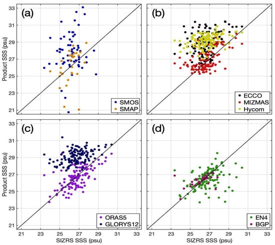
Figure 5.
Scatter diagrams of sea surface salinity (SSS) of SIZRS (2 m) to (a) satellite missions, and of SIZRS (5 m) to (b,c) ocean model simulations, and (d) in–situ observations during SIZRS AXCTD drops. Black line signifies equivalent salinity values (psu).
Table 2.
Statistical analysis including the total drop average, the average difference, the correlation coefficient, and the p-value of sea surface salinity (psu) between SIZRS other salinity products at each SIZRS drop point.
The average salinity difference from in situ to satellites was higher in SMOS than in SMAP. SMAP had a stronger correlation to SIZRS at 2 m, but both satellites’ salinity data had higher p-values, implying they are not statistically significant (p-values > 0.05). The ocean models, ECCO, HYCOM, and GLORYS12 similarly yielded higher salinities (greater than 2.2 higher average psu) and moderate correlations (correlation coefficients < 0.6) with in situ observations in the BG region. ORAS5 had the salinities closest to SIZRS, within 0.06 psu difference on average, and the strongest correlation with SIZRS at 0.612.
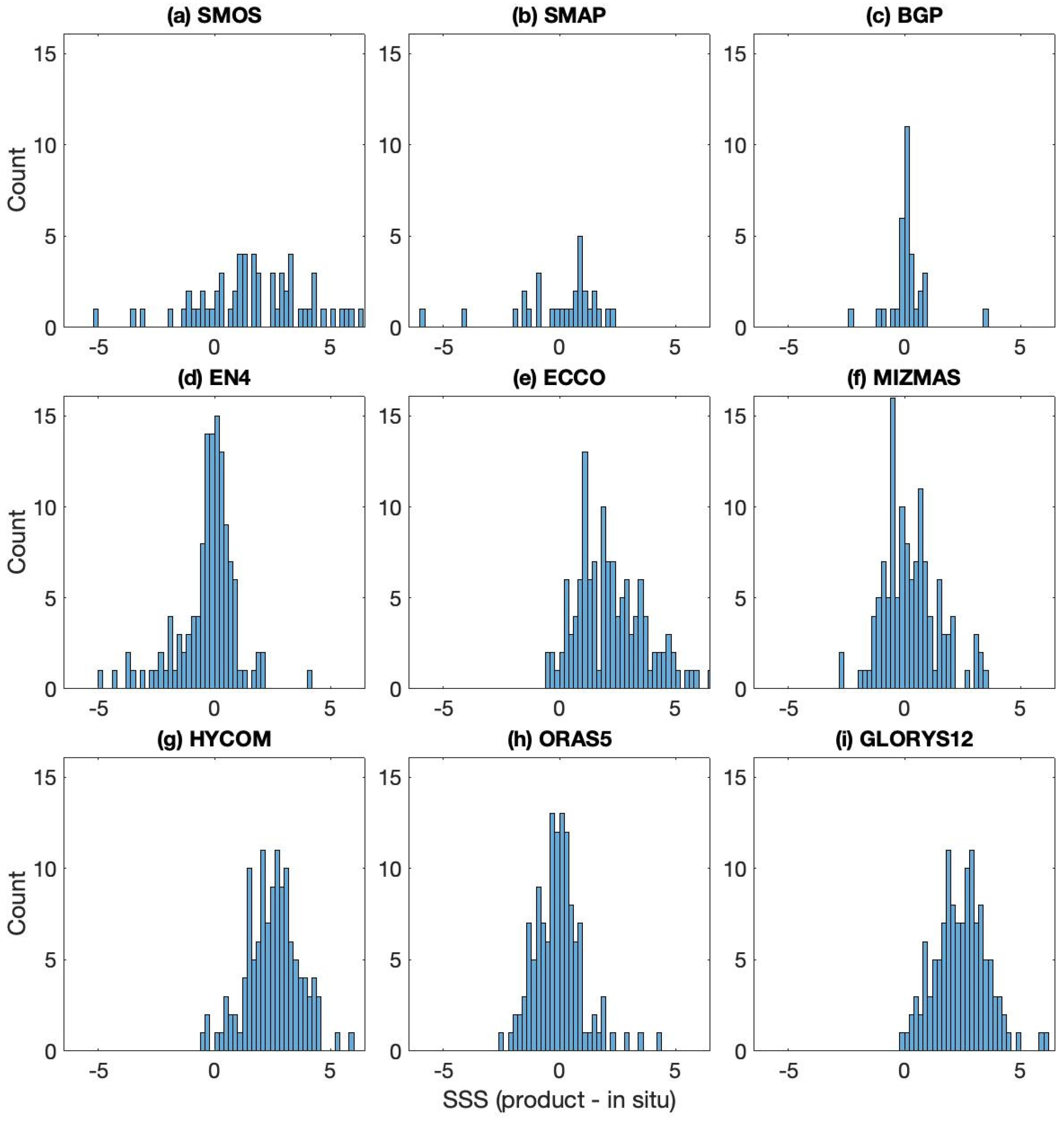
The distribution of SSS differences of products minus SIZRS measurements were further analyzed through histograms, illustrated in Figure 6, to observe the distribution of product salinities from SIZR salinities at each SIZRS drop. The frequency of samples was distributed in 0.2 psu bins.
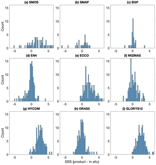
Figure 6.
Histograms of sea surface salinity (SSS) differences (psu) of products minus in situ (SIZRS). SIZRS at 2-m is used for (a,b) Satellites, and 5-m for (c,d) in situ and (e–i) models. Bin widths are 0.2 psu.
Satellite products (Figure 6a,b) showed departures from SIZRS salinities that vary widely. SMOS SSS data distributions are similar to SMAP, but with the majority of departures from SIZRS salinity being positive and a few outliers of large negative salinity differences. Salinity differences of SMOS relative to SIZRS are generally 1 psu higher than those of SMAP (Table 3). However, SMAP’s bias was overall negative, which can be linked to the few large negative outliers (Figure 6b). The satellite remotely sensing SSS had the largest standard deviations from SIZRS SSS compared to other products, specifically in SMOS (~2.33 psu). Their variability compared to SIZRS salinity would be a consequence of the larger overall variability of the remote sensing SSS (Figure 4).
Table 3.
Median, mean, standard deviation (Std. Dev.), and Root Mean Square Deviation (RMSD) of SSS differences between products and SIZRS in situ data at each latitude SIZRS measurements were taken.
BGP observations were similar to SIZRS, but like the satellite product, compared to SIZRS, BGP has fewer samples with which to make definitive conclusions. In contrast to other products, the majority of salinity values from EN4 are fresher than SIZRS, with an average bias of −0.27 psu. In situ products showed close relation to SIZRS in average salinity. However, EN4 had a relatively high standard deviation, and a greater root mean square deviation (RMSD) from SIZRS than BGP. The RMSD signifies the accuracy measurement between the observed salinity and the SIZRS, where an RMSD of 0 would indicate a perfect comparison fit. This helped to delineate difference extremes rather than solely focusing on the average of the estimations.
When comparing models to SIZRS, GLORYS12, HYCOM, and ECCO contain more saline values with average biases greater than 2 psu and have the largest RMSD of the ocean models at 2.89 psu, 2.73 psu, and 2.63 psu, respectively. ECCO salinity departures from SIZRS salinities have the highest standard deviation (1.47 psu) compared to the other models. HYCOM and GLORYS 12 showed the greatest average disagreement with SIZRS salinity compared to all products with a bias of about 2.50 psu and 2.44 psu, respectively. MIZMAS and ORAS5 salinity anomalies relative to SIZRS are more centered around 0 psu, with ORAS5 showing the closest comparison to SIZRS as the only ocean model indicating a fresher bias (−0.052) and a closer relation with an RMSD of 1.05.
Since the SIZRS drops differ spatially as well as temporally, we next average the data along the transect (150°W from 70.5°N–80.5°N) to show the monthly average sea surface salinities between products on a timeline basis in Figure 7.
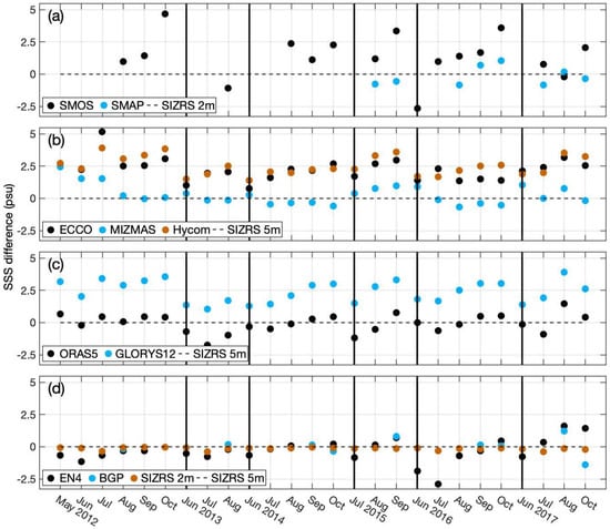
Figure 7.
Sea surface salinity (SSS) differences (psu) from SIZRS (at 5 m) averaged along (150°W from 70.5°N–80.5°N) compared to (a) satellite missions, (b,c) ocean model simulations, and (d) in–situ observations. Grey, vertical lines separate years where months are not consecutive.
Differences in product salinities from SIZRS SSS revealed monthly patterns between instruments and estimations (Figure 7). Satellite salinity differences from SIZRS tended to become more saline in later months, perhaps because the initial advance of the ice edge obscured the lowest salinities near the center of the BG. This pattern also held true for the models, where early months showed lower and fresher SSS differences, as opposed to later months where the differences were heightend and typically more saline than SIZRS. Compared to ECCO and HYCOM, the salinities of MIZMAS were less than SIZRS through many of the monthly means, especially during 2014 and 2016 (Figure 7b). GLORYS12 and ORAS5 had common patterns of local salinity variations throughout time, but GLORYS12 consistently showed higher salinity values at about 2.3 psu on average compared to ORAS5 and 2.5 psu compared with SIZRS (Figure 7c). On the other hand, ORAS5 SSS fluctuated between more saline or fresher estimations than SIZRS measurements. Differences between EN4 and SIZRS monthly averages stayed between 1 psu, except for June and July 2016 observations.
3.2. Vertical Salinity Structure
The vertical structure of the upper ocean defines changes in mixed layer depth, FWC, and stratification in the BG. We analyzed salinity within the water column between 2012 and 2017 from EN4 and ocean models averaged along the 150°W BG transect between 70.5°N and 80.5°N (Figure 8).
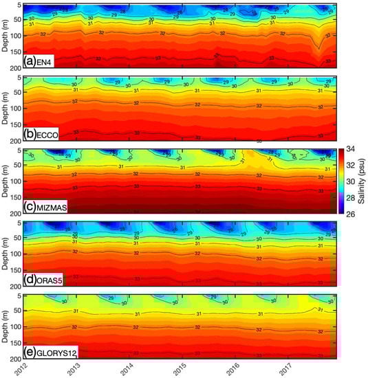
Figure 8.
Contours of salinity (psu) averaged along 150°W between 70.5°N and 80.5°N, as a function of depth and time from 2012–2017.
We examined salinity from 5 m to 200 m to include the mixed layer, usually shallower than 55 m in the BG region, and the main part of the upper ocean halocline. Seasonality between the EN4 data and ocean models is illustrated by the declining salinities throughout the summer into autumn months. MIZMAS salinity differences between the surface and 200 m were the greatest of all the models with surface salinities under 27 psu and nearly 34 psu at 200 m. ORAS5 showed the closest relationship in seasonal variations to EN4. Contrarily, ECCO and GLORYS12 indicated the lowest vertical gradients in salinity. Also, their surface salinities during autumn, when the annual salinity is lowest, were continuously higher than other products.
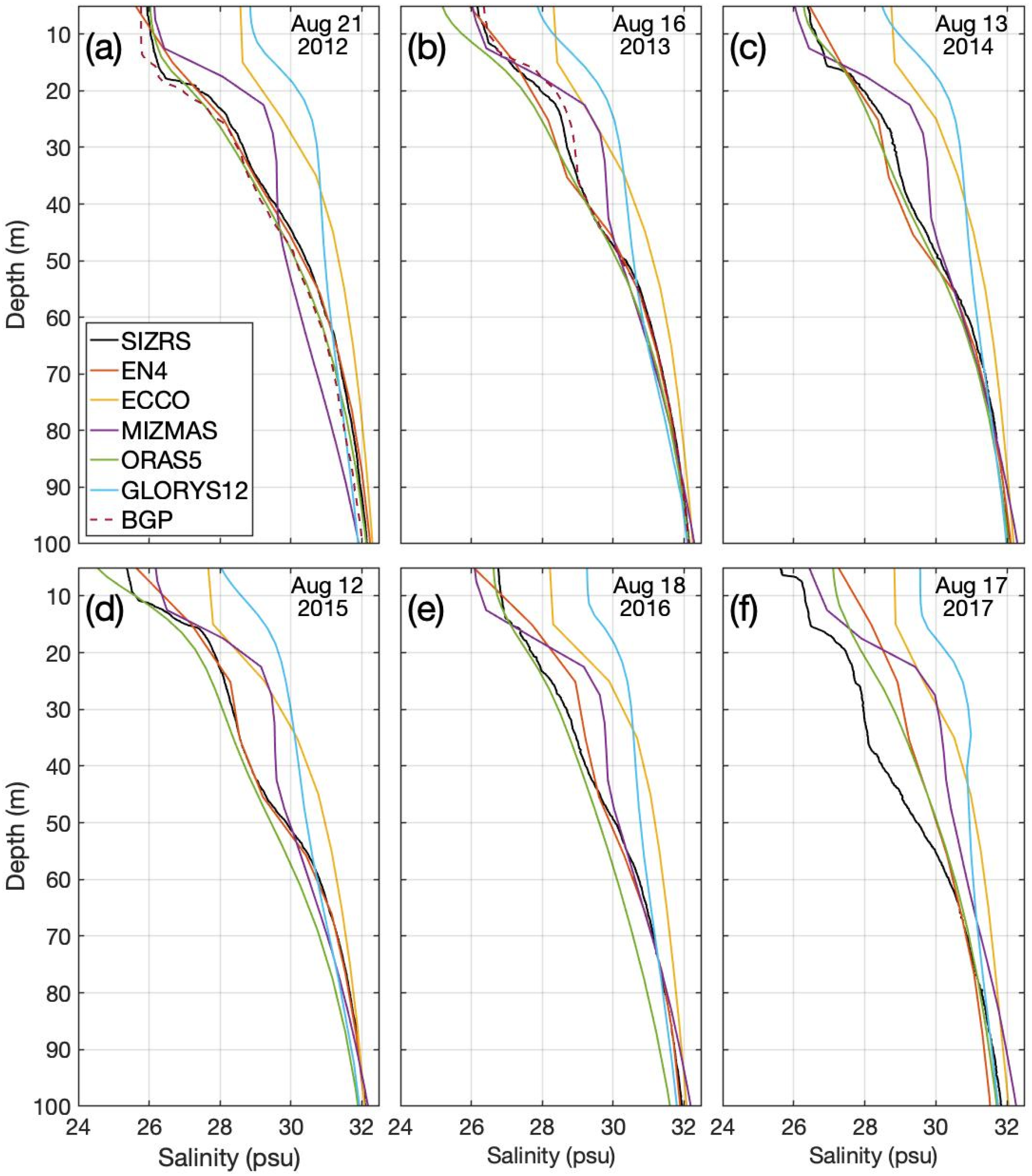
To directly compare these models to SIZRS, we provide snapshots of the specific August dates of each year averaged along the 150°W transect with BGP, EN4, and model estimations to the closest temporal resolution possible, ranging from daily to monthly data (Figure 9). Depth profiles above 100 m show large salinity differences among the products.
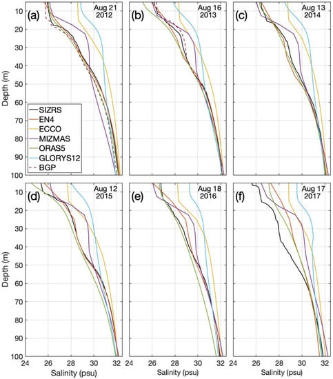
Figure 9.
Salinity (psu) depth profile comparisons of SIZRS drops with other products over the transect average (150°W, 70.5°N–80.5°N) during (a) 21 August 2012, (b) 16 August 2013, (c) 13 August 2014, (d) 12 August 2015, (e) 18 August 2016, (f) 17 August 2017.
The in situ observations from BGP (Figure 9a,b) and EN4 closely matched SIZRS drops, although the slope of EN4 is smoothed with depth, and the mixed layer was not as distinguishable in the ECCO salinity profiles. Of the models, ORAS5 had the closest relation to SIZRS throughout the depth profiles, whereas GLORYS12 and ECCO were consistently higher than SIZRS with depth. MIZMAS salinity difference from SIZRS salinity was greatest between depths of about 20 m to 50 m. The mixed layer depth appeared in most products around 16 m, separating the fresher waters and sea ice cover from the more saline waters below. ECCO salinity is just under 29 psu at depths less than 15-m, at which depth it increases logarithmically. GLORYS12 was similar to ECCO with higher SSS; however, its halocline is not as pronounced as other products that showed large increases in salinity around the bottom of the mixed layer depth (~20 m).
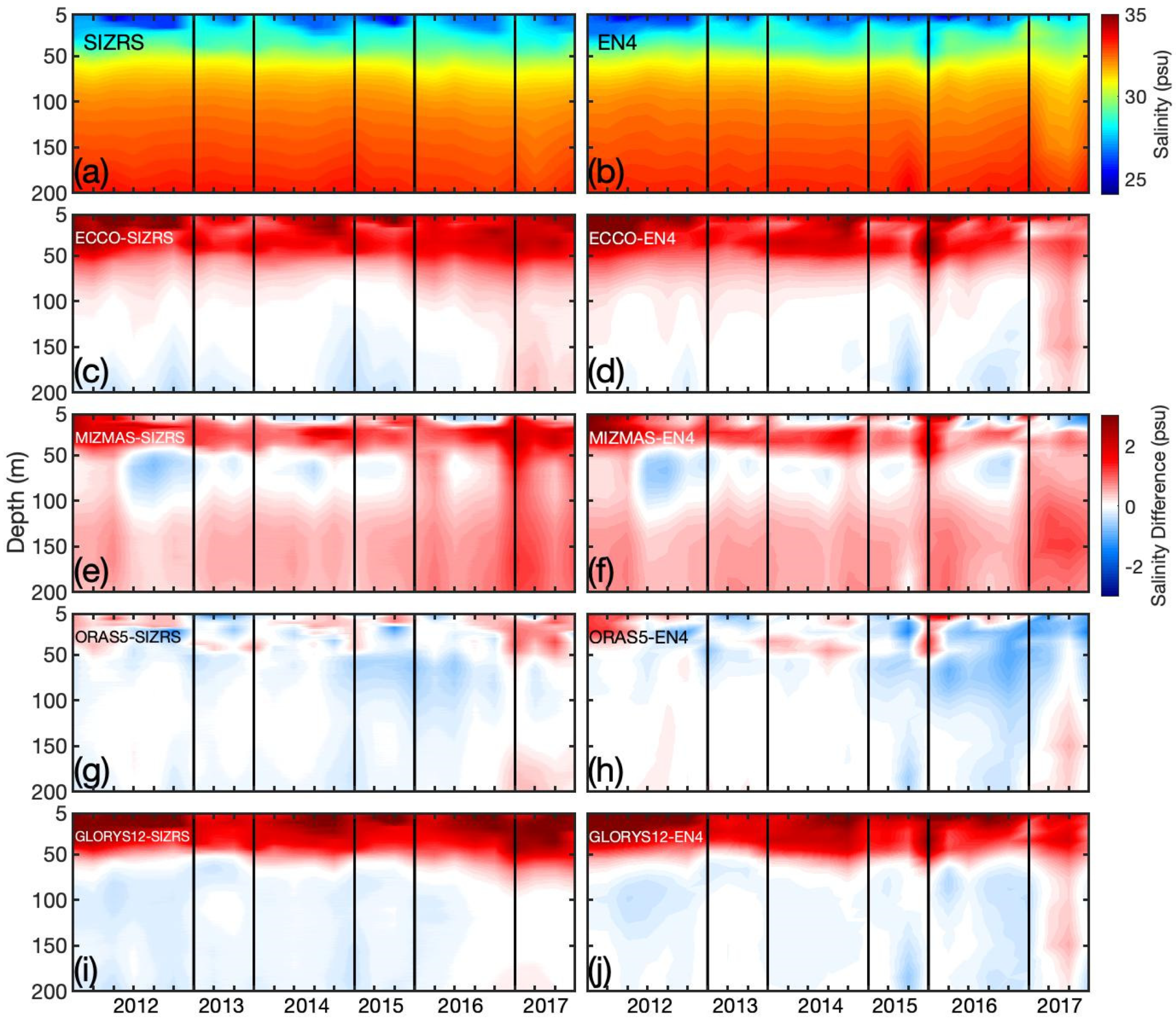
To further distinguish the salinity profile differences between products, we took the average of SIZRS, EN4, and ocean model simulations where individual SIZRS latitude measurements were taken along 150°W in the BG during each available month (Figure 10).

Figure 10.
Salinity (psu) versus depth profiles averaged monthly over all SIZRS latitudes for (a) SIZRS and (b) EN4 from 2012–2017, and the departure of salinity from SIZRS (left column) and EN4 (right column) for the ocean models (c,d) ECCO, (e,f) MIZMAS, (g,h) ORAS5, and (i,j) GLORYS12. Grey, vertical lines separate years where months are not consecutive.
Salinity contours from SIZRS and EN4 (Figure 10a,b) illustrate the vertical salinity structure of monthly averages at all SIZRS drops. With small exceptions, these two in situ products are very similar, with low salinities (~26 psu) above 25 m and showing salinities reaching 31 psu by 60 m. ECCO and GLORYS12 showed relatively higher salinity (over 2 psu) in the surface layer, but their differences with respect to SIZRS and EN4 sharply decreased below 60 m. MIZMAS showed salinities close to in situ values at the surface, but higher biases occurred between the 10 m and 50 to 60 m depth layers. Unlike other models, MIZMAS simulates higher salinities with 0.5–1 psu differences below 100 m depth. ORAS5 depth-profiles are overall very similar to SIZRS and EN4 but are slightly (higher) lower in 2017 when compared to SIZRS (EN4).
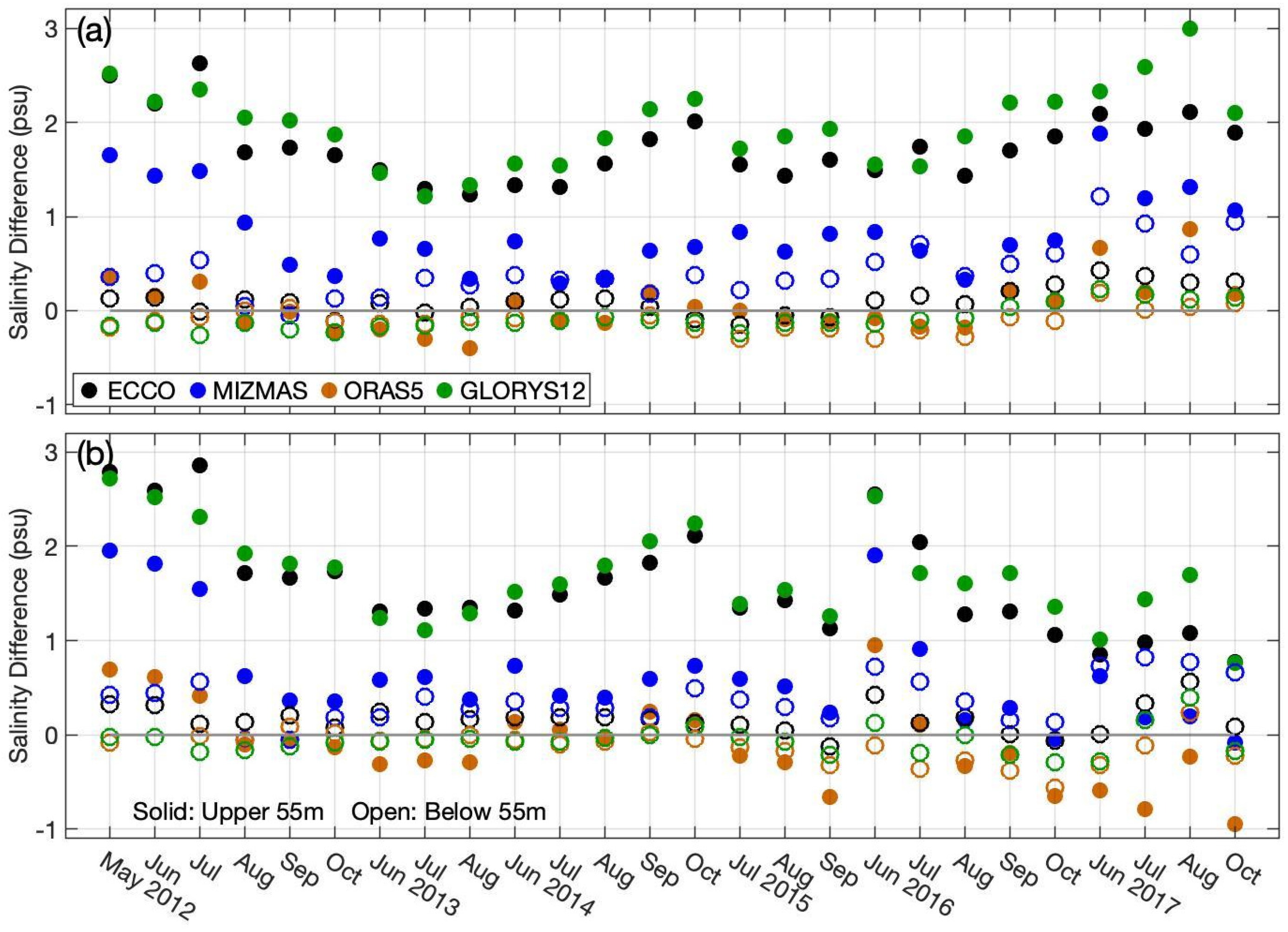
Overall, the greatest differences among the products were in the upper region of the water column above a 50 m depth, a region most important when analyzing the freshwater budget in the BG region. Therefore, to inspect model comparisons between the vertical layers where we saw the highest and lowest differences, we separated comparisons between an upper region (5 m–55 m) and lower region (55 m–207 m) in Figure 11. Depths of products are integrated to a 207 m depth as it is the EN4 product’s depth layer closest to 200 m, as distinguished in previous figures.
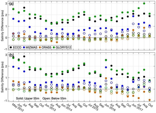
Figure 11.
Differences in salinity (psu) depth profiles of each product at each SIZRS latitude averaged monthly from 2012–2017 separated by vertically-averaged (solid dot) upper 5 m to 55 m region and the (opened dot) lower 55 m to 207 m region for (a) model minus SIZRS, and (b) model minus EN4.
Statistical analyses are described in Table 4, including standard deviations, RMSD, and average differences (or bias) from SIZRS and EN4 products for the upper region compared to the lower region averages. Upper region averages have positive differences between the models and both SIZRS and EN4, except for ORAS5, which fluctuated between positive and negative salinity differences and had the smallest bias to both in situ products. However, for salinity differences in the lower regions, GLORYS12 data was closest to SIZRS, and MIZMAS data were closest to EN4.
Table 4.
Standard deviation of salinity (psu) profile differences between model minus in situ (SIZRS and EN4) products for the upper region (above 55 m depth) and lower region (below 55 m depth).
Table 4 also highlights that the discrepancy between products was more concentrated in the upper region than the lower. The largest RMSD, representing a higher magnitude of errors, occurs with GLORYS12 in the upper region for both SIZRS and EN4, and in MIZMAS when comparing the lower region of both in situ products. This stresses the importance of analyzing salinity features in the upper region of the BG and the Arctic Ocean when evaluating critical characteristics or changes in the halocline structure and its influences, and the oceans’ vertical circulation dynamics.
3.3. Freshwater Content
FWC as a measure of depth-integrated salinity anomaly per unit area indicates where FW is accumulating or decreasing in the Arctic Ocean. Different assimilation techniques and forcing between models influence the salinity estimates and FWC in turn. We interpolated salinity anomaly relative to 34.8 psu of each model into 1° × 1° grided data and calculated the accumulated depth FWC (Equation (1)) across the Arctic Ocean between 5 m and 500 m, averaged from 2012–2017 as seen in Figure 12.
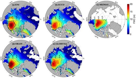
Figure 12.
Freshwater content (FWC; m) from 5 m–500 m depth in the Arctic Ocean and averaged between 2012–2017 from the (a) EN4 data and five models: (b) ECCO, (c) MIZMAS, (d) ORAS5, and (e) GLORYS12. FWC is contoured every 2 m with a reference salinity of 34.8 psu. Beaufort Gyre region is outlined in a black box (Figure 12a).
As expected, low FWC comprises the more saline regions on the Atlantic side of the Arctic Ocean, whereas the Canadian Basin and Canadian Archipelago contain more FW for all models, especially in the BG region and the Davis Strait. The peak FWC was lowest in ECCO, between 16 m and 17 m on average between 2012–2017 (Figure 13b). MIZMAS and GLORYS12 maximum FWC was slightly greater than 18 m in the BG, whereas EN4 and ORAS5 showed at least 20 m of FWC in the Arctic Ocean during that period. EN4 showed between 11 m and 12 m of FWC in the Davis Strait region. ECCO and GLORYS12 showed moderate levels of FWC in the Davis Strait, whereas ORAS5 did not. ORAS5 agreed well with the SIZRS FWC of 22.09 m averaged along the 150°W and integrated from 5.02 m to 435.65 m, its minimum sampled depth.
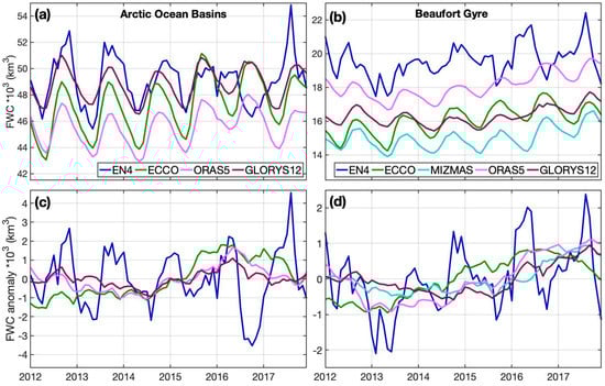
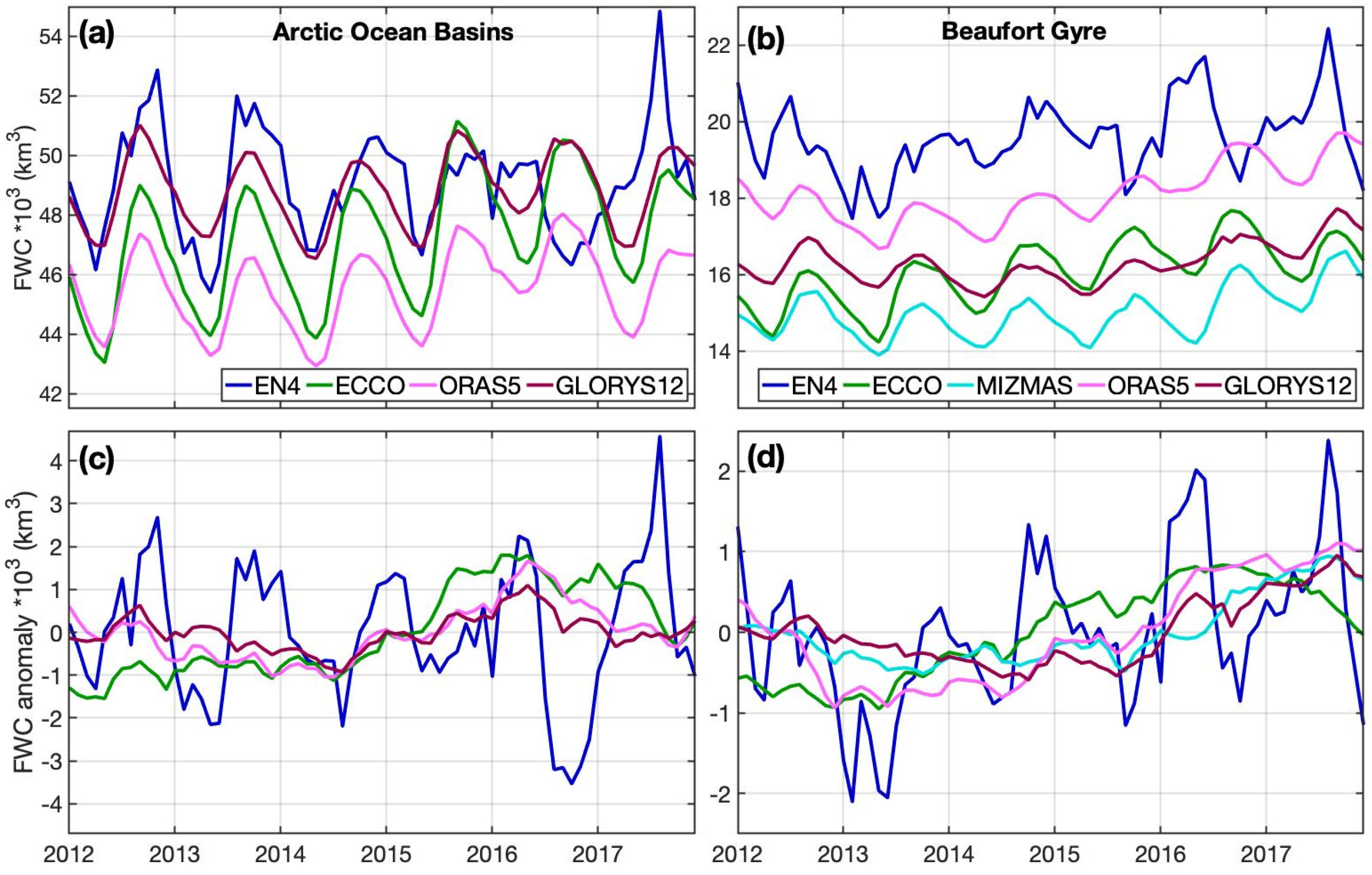
Figure 13.
Timeseries of depth-integrated (5 m–500 m) and box–accumulated freshwater content (FWC; km3) in the (a,c) Arctic Ocean Basins (180°W–180°E, 67°N–90°N) and the (b,d) Beaufort Gyre (170°W–130°W, 70.5°N–80.5°N) from (top panel) raw data and the (bottom panel) departure from the monthly climatology between 2012 and 2017.
We next compared the box–accumulated FWC [km3] of the Arctic Ocean deep basin, which encompassed areas with depths greater than 500 m, and the BG region to analyze the seasonal and interannual oscillations between 2012–2017 for each model (Figure 13). The FWC from MIZMAS was restricted between 180°W–80°W in the Arctic Ocean due to the geographic limits of the model; therefore, we excluded it from the Arctic Basin FWC calculations.
FWC seasonality is induced by runoff, precipitation, sea ice melt, or growth combined with seasonal wind-driven circulation changes. The ocean models expressed a switch from mostly negative to mostly positive anomalies by 2015 in the Arctic Basin and 2016 in the BG. Overall trends of FWC were not statistically significant during 2012–2017. Seasonal variations of FWC from the models were relatively consistent. Averages and standard deviations of the FWC time series for the Arctic Basin and BG are given in Table 5.
Table 5.
Statistical analysis of averages (avg.) and standard deviations for FWC in the Arctic Basin and the Beaufort Gyre are depicted in Figure 13.
From 2003–2009, during the transition to a more cyclonic mode, Morison et al. [5] SI–7 (Freshwater Content Rate–of–Change Comparisons) found the total freshwater of the deep Arctic Ocean increased to 804 km3 year−1 or 0.0255 × 10⁴ m3 s−1 = 0.0255 Sverdrup, almost equal to the rate of sea ice loss but much smaller than the difference between BG and Eurasian Basin freshwater change. The BG minimum FWC in 2013 from all products except for GLORYS12 coincides with Proshutinsky et al. [34].
Perhaps the most interesting feature was the behavior of EN4 Beaufort Gyre FWC in 2016, during which it rose out of phase with the models in the first part of the year and then, still out of phase, dropped during the summer. At the same time, the EN4 Arctic Ocean FWC remained unusually constant over much of 2016, suggesting a redistribution of freshwater from outside the BG into the BG in the winter and spring of 2016. Overall, the products express a greater range of differences in average FWC, greater than the seasonal variations.
4. Discussion
4.1. Sea Surface Salinity
We used SMOS produced by BEC, which, as Xie et al. [35] shows, has a lower bias relative to in situ data in the BG area than alternative SMOS products. Despite having a lower temporal and spatial resolution than SMOS, SMAP showed more promising outcomes than SMOS along the BG 150°W transect, where it has a lower salinity bias than SIZRS data [36,37,38]. Bingham et al. [38] found higher bias in SMOS BEC than in SMAP and EN4. Fournier et al. [36] said that SMAP RSS and SMOS BEC had lower RMSD relative to in situ than other SMAP and SMOS products. Between the satellite products, SMOS BEC had the lowest positive bias of (0.08). When comparing missions between 60°S–60°N, Bao et al. [37] found a higher bias in SMOS (−0.113) than SMAP (−0.078). Nonetheless, satellites show small SSS correlation values compared with SIZRS observations, most likely due to the small sample size and low spatial coverage obtained.
All ocean models, except for ORAS5 and MIZMAS, have transect averages SSS greater than EN4. Carton et al. [39] compared ORAS5 and earlier versions of ECCO (version 4, release 3) and EN4 (version 1.1) on a global scale as well as parts of the Arctic Ocean. Their results confirm closer comparisons between salinity estimations from ORAS5 and EN4 compared to ECCO and EN4. Through the analysis of transect averaged SSS, MIZMAS demonstrated the largest range of seasonal salinity fluctuations with higher winter values comparable to GLORYS12 and near equivalent summer month salinities to in situ products. MIZMAS forcing also incorporated monthly climatology of freshwater from river discharge into the Arctic Ocean and Bering Strait, to which we can attribute the lower salinity values viewed in spatial maps near the mouth of the Mackenzie River, the Canadian Archipelago, and the Chukchi Sea [40].
Compared to SIZRS data, ORAS5 had the highest correlation coefficient (0.612), suggesting a higher accuracy in salinity estimates in the BG despite having a lower temporal resolution than other models. ORAS5 and ECCO shared the same ERA-Interim surface forcing fields and surface flux bias correction [39]. Yet, these two products showed differing distributions in histograms of salinity differences from SIZRS, where the direction of outliers for ORAS5 (ECCO) was negative (positive). ORAS5 and GLORYS12 share the same NEMO model component, but GLORYS12 produced correlations coefficients (0.406) and higher bias (2.437 psu) relative to SIZRS, signifying that ORAS5 is moderately correlated to in situ data and GLORYS12 is not. When analyzing the monthly averages of salinity differences between products and SIZRS along the BG transect, most models tend to overestimate salinity near the end of each year.
This study emphasizes the importance of SSS product comparisons between satellite data and ocean model estimations in an area where in situ observations are abundant compared to the observation-poor Arctic regions like the Russian shelf. While satellite observations are restricted by the extent of sea ice in the Arctic Ocean, their averaged annual coverage extends over the East Siberian shelf (Figure 2). The bias and regional discrepancies shown by these products help to discern their advantages and disadvantages when analyzed in other regions of the Arctic Ocean. The scarcity of in situ measurements in portions of the Arctic Ocean that contribute to the overall analysis of the Arctic Ocean revealed the significance of improved remote sensing techniques and ocean model development.
4.2. Vertical Salinity Structure
Depth profile analysis in this study highlights the variability at depths shallower than 55 m and between 55 and 207 m for deeper layer comparisons. Past research has commonly defined the mixed layer depth as the depth where the density increase above the mixed layer reaches 0.25 kg/m3, which is consistently deeper than 10 m in the BG and can reach 30 m in the winter [34,41,42]. In contrast, Jackson et al. [43] emphasize that the alteration of the upper 100 m of the Canadian Basin has been influenced by heightened temperatures and freshwater levels where the mixed layer depth during winter months shoaled from 50 m prior to the 1970s to around 24 m more recently.
Seasonality of salinity-in-depth profiles, where the melting of sea ice during the summer causes surface freshening and stronger salinity gradients, is seen best in EN4 and ORAS5 compared to GLORYS12. ECCO shows a similar structure to GLORYS12; however, ECCO retains slightly fresher surface waters longer each year. Except for ORAS5, comparisons among the other three models varied, but they all maintained slightly higher salinities with depth compared to SIZRS. GLORYS12 (MIZMAS) had the highest bias in the upper (lower) region compared to SIZRS and EN4.
4.3. Freshwater Content
FWC analysis is vital to the understanding of the distribution and key role of salinity in the Arctic Ocean. Serreze et al. [44] analyzed Arctic FWC, finding less in the central Arctic and more accumulating in the Eurasian basin, such as the Kara and Laptev Seas. Wang et al. [45] found that the FWC in the Canadian basin increased upwards of 5 m between 2004 and 2009, with a less significant difference between 2009 and 2015. The BG region accounts for about a fourth of the total liquid FWC, with a current peak between ~17 m for ECCO to ~21 m shown in EN4.
FWC from model estimations in our study also agreed with Proshutinsky et al. [4] in that the BG seasonal changes of total FWC accounted for about 5% of its total volume, even for the current period, which they attribute to atmospheric circulation. EN4 estimated the FWC of the BG to be slightly higher than 22 × 103 km3 during 2017, whereas the other models except for ORAS5 (just shy of 20 × 103 km3) estimated lower than 18 × 103 km3 throughout the timeline. The largest seasonal change of FWC from the EN4 data occurred near the end of 2017, decreasing at least 4.1 × 10³ km3, attributing to a departure of more than 3 × 10³ km3 from its monthly BG climatologies. The 2012 FWC anomalies in Figure 13c,d for the BG are slightly smaller, but similar to estimates shown by Rabe et al. [46]. However, these slight differences from Rabe et al. [46] can be credited to the use of a different model and their reference salinity of 35 psu instead of our 34.8 psu. The products do not show as great a seasonal difference in FWC as in their annual averages in the Arctic basin. The overall trend of FWC for the Arctic Ocean had relatively stabilized in the decade following 2010, between the relative balance of the BG freshening and the reduction of FW in the rest of the Arctic Ocean, especially in the Eurasian Basin, which Morison et al. [5] attributes over the long term to the changes in surface circulation governed by the positive shift of the Arctic Oscillation in recent decades [47].
5. Conclusions
This study primarily focuses on salinity comparisons between numerous salinity products commonly used in the Arctic Ocean and sub-Arctic seas. Large-scale SSS characteristics between these products are similar. However, important regions like the BG that provide insight into the state of the changing Arctic Ocean in a warming climate, show concerning dissimilarities. Present research has shown that over the past three decades, the Arctic Ocean surface circulation has been dominated by a more dominant cyclonic mode associated with higher average vorticity, advection of more Eurasian runoff into the Canadian Basin, enhanced divergence and thinning of the ice cover, and in principle more FW release [5]. The changes we see in the Beaufort Gyre in recent years are embedded in the larger and longer scale change. Therefore, we have conducted a model–observation analysis of surface and depth profiles of salinity variations from 2012 to 2017 in the BG area. The satellite missions of SMOS, SMAP, and OISSS, combined with the Arctic Ocean model simulations from ECCO, MIZMAS, HYCOM, ORAS5, and GLORYS12, show a range of biases when compared to the in situ products of SIZRS surveys, BGP CTD casts, and the EN4 data.
In the BG area, SMAP shows more promising SSS comparisons to in situ data than SMOS. Ocean models evaluated in this study, except for ORAS5, tend to overestimate in situ SSS, with the largest positive bias represented by HYCOM at about 2.5 psu. ORAS5 provides the strongest positive correlation coefficient (0.612) and lowest salinity bias relative to observations. GLORYS12 salinity depth profiles above 55 m differ most from in situ data but are closest to SIZRS when comparing salinities between the 55 m and 207 m region. From 55 m to 207 m, MIZMAS shows higher biases relative to observations. FWC trends in the Arctic basin and the BG were insignificant between 2012 and 2017. The seasonal FWC differences between ocean models and EN4 were not as great as when comparing their averaged annual FWC. Future sea ice melt will contribute even more to the accumulation of FW to the BG that can be eventually released to adjacent seas if it does not form back into sea ice the following winter.
Author Contributions
Conceptualization, B.S.; methodology, S.B.H.; software, S.B.H.; validation, B.S., S.B.H. and J.H.M.; formal analysis, S.B.H., B.S. and J.H.M.; investigation, S.B.H., B.S. and J.H.M.; resources, B.S.; data curation, B.S. and S.B.H.; writing, S.B.H.; visualization, S.B.H., B.S. and J.H.M.; supervision, B.S.; funding acquisition, B.S. All authors have read and agreed to the published version of the manuscript.
Funding
This research was funded by the United States Office of Naval Research Awarded #N00014-20-1-2680, awarded to B.S.
Institutional Review Board Statement
Not applicable.
Informed Consent Statement
Not applicable.
Data Availability Statement
SMOS BEC V3.1 3day data at 25km resolution were produced by the Barcelona Expert Centre (http://bec.icm.csic.es, accessed on 3 April 2021) a joint initiative of the Spanish Research Council (CSIC) and Technical University of Catalonia (UPC), mainly funded by the Spanish National Program on Space and is available through a secure FTP server: sftp://becftp.icm.csic.es:27500, accessed on 4 April 2021. SMAP SSS V4.0 Level 3 is a 0.25° gridded product with 8–day running mean salinity data obtained from RSS (www.remss.com/missions/smap/salinity/), accessed on 3 April 2021. Multi-mission OISSS 4–day 0.25° L4v1 gridded salinity data were downloaded from the JPL/PO.DAAC drive (https://podaac.jpl.nasa.gov/dataset/OISSS_L4_multimission_7day_v1), accessed on 10 September 2021. SIZRS data is provided by the Polar Science Center along the 150°W transect on monthly expeditions anywhere between May and October 2012–2017 (http://psc.apl.uw.edu/research/projects/sizrs/data-2/), accessed on 6 April 2021. The Woods Hole Oceanographic Institution (WHOI) Beaufort Gyre Exploration Project (BGEP) provides monthly observations from CTD casts along the BG 150°W transect (https://www2.whoi.edu/site/beaufortgyre/data/ctd-and-geochemistry/), accessed on 3 June 2021. EN.4.2.1 monthly salinity data at a 1° horizontal resolution with 42 vertical layers since 1900 were obtained from https://www.metoffice.gov.uk/hadobs/en4/, accessed on 20 April 2021, and are © British Crown Copyright, Met Office, provided under a Non–Commercial Government License (http://www.nationalarchives.gov.uk/doc/non-commercial-government-licence/version/2/), accessed on 3 April 2021. ECCO v4r4 daily salinity data with an LLC90 grid special resolution between 22 km–110 km were downloaded from the JPL/PODAAC ECCO drive (https://ecco.jpl.nasa.gov/drive/files/Version4/Release4/nctiles_daily), accessed on 22 February 2021. MIZMAS daily 3D salinity data with 40 depth layers were provided through a private server with a horizontal resolution of about 20 km, accessed on 23 July 2021. Daily SSS data from HYCOM + CICE is averaged from 12–h data and obtained from coupled on the same 1/12° global tripole grid and obtained from OPeNDAP framework (https://www.hycom.org/dataserver), accessed on 16 April 2021. ORAS5 monthly salinity data were taken from the University of Hamburg at 0.25° resolution and are available from 1993–2019 (https://icdc.cen.uni-hamburg.de/thredds/catalog/ftpthredds/EASYInit/oras5/ORCA025/vosaline/catalog.html) accessed on 13 April 2021. Daily salinity data from GLORYS12 version 1 with a 1/12° horizontal resolution and 50 vertical depth levels are available by the CMEMS server from 1993–2019 (ftp://my.cmems-du.eu/Core/GLOBAL_REANALYSIS_PHY_001_030/global-reanalysis-phy-001-030-daily), accessed on 3 April 2021.
Acknowledgments
We are thankful for the helpful comments of the two anonymous reviewers, which improved the quality of this paper.
Conflicts of Interest
The authors declare no conflict of interest.
References
- Fournier, S.; Lee, T.; Wang, X.; Armitage, T.W.K.; Wang, O.; Fukumori, I.; Kwok, R. Sea Surface Salinity as a Proxy for Arctic Ocean Freshwater Changes. J. Geophys. Res. Oceans 2020, 125, e2020JC016110. [Google Scholar] [CrossRef]
- Krishfield, R.A.; Proshutinsky, A.; Tateyama, K.; Williams, W.J.; Carmack, E.C.; McLaughlin, F.A.; Timmermans, M.-L. Deterioration of perennial sea ice in the Beaufort Gyre from 2003 to 2012 and its impact on the oceanic freshwater cycle. J. Geophys. Res. Oceans 2014, 119, 1271–1305. [Google Scholar] [CrossRef]
- Proshutinsky, A.; Johnson, M.A. Two circulation regimes of the wind-driven Arctic Ocean. J. Geophys. Res. Space Phys. 1997, 102, 12493–12514. [Google Scholar] [CrossRef]
- Proshutinsky, A.; Krishfield, R.; Timmermans, M.-L.; Toole, J.; Carmack, E.; McLaughlin, F.; Williams, W.J.; Zimmermann, S.; Itoh, M.; Shimada, K. Beaufort Gyre freshwater reservoir: State and variability from observations. J. Geophys. Res. Space Phys. 2009, 114, C00A10. [Google Scholar] [CrossRef]
- Morison, J.; Kwok, R.; Dickinson, S.; Andersen, R.; Peralta-Ferriz, C.; Morison, D.; Rigor, I.; Dewey, S.; Guthrie, J. The Cyclonic Mode of Arctic Ocean Circulation. J. Phys. Oceanogr. 2021, 51, 1053–1075. [Google Scholar] [CrossRef]
- Morison, J.; Kwok, R.; Peralta-Ferriz, C.; Alkire, M.; Rigor, I.; Andersen, R.; Steele, M. Changing Arctic Ocean freshwater pathways. Nat. Cell Biol. 2012, 481, 66–70. [Google Scholar] [CrossRef] [PubMed]
- Haine, T.W.N.; Curry, B.; Gerdes, R.; Hansen, E.; Karcher, M.; Lee, C.; Rudels, B.; Spreen, G.; de Steur, L.; Stewart, K.D.; et al. Arctic freshwater export: Status, mechanisms, and prospects. Glob. Planet. Chang. 2015, 125, 13–35. [Google Scholar] [CrossRef] [Green Version]
- De Steur, L.; Steele, M.; Hansen, E.; Morison, J.; Polyakov, I.; Olsen, S.M.; Melling, H.; McLaughlin, F.A.; Kwok, R.; Smethie, W.M.; et al. Hydrographic changes in the Lincoln Sea in the Arctic Ocean with focus on an upper ocean freshwater anomaly between 2007 and 2010. J. Geophys. Res. Oceans 2013, 118, 4699–4715. [Google Scholar] [CrossRef] [Green Version]
- Aagaard, K.; Carmack, E.C. The role of sea ice and other fresh water in the Arctic circulation. J. Geophys. Res. Space Phys. 1989, 94, 14485–14498. [Google Scholar] [CrossRef]
- Carmack, E.; McLaughlin, F.; Yamamoto-Kawai, M.; Itoh, M.; Shimada, K.; Krishfield, R.; Proshutinsky, A. Freshwater Storage in the Northern Ocean and the Special Role of the Beaufort Gyre; Springer: Singapore, 2008; pp. 145–169. [Google Scholar]
- Fuentes-Franco, R.; Koenigk, T. Sensitivity of the Arctic freshwater content and transport to model resolution. Clim. Dyn. 2019, 53, 1765–1781. [Google Scholar] [CrossRef] [Green Version]
- Dewey, S.R.; Morison, J.H.; Zhang, J. An Edge-Referenced Surface Fresh Layer in the Beaufort Sea Seasonal Ice Zone. J. Phys. Oceanogr. 2017, 47, 1125–1144. [Google Scholar] [CrossRef]
- Meissner, T.; Wentz, F.J.; Manaster, A.; Lindsley, R. Remote Sensing Systems SMAP Ocean Surface Salinities Level 3 Running 8-Day, Version 4.0 Validated Release. Remote Sensing Systems. Santa Rosa, CA, USA. Available online: www.remss.com/missions/smap/salinity/ (accessed on 3 April 2021).
- Meissner, T.; Wentz, F.J.; Le Vine, D.M. The Salinity Retrieval Algorithms for the NASA Aquarius Version 5 and SMAP Version 3 Releases. Remote Sens. 2018, 10, 1121. [Google Scholar] [CrossRef] [Green Version]
- Melnichenko, O.; Hacker, P.; Potemra, J.; Meissner, T.; Wentz, F. Aquarius/SMAP Sea Surface Salinity Optimum Interpolation Analysis. IPRC Technical Note No. 7. 2021. Available online: https://podaac-tools.jpl.nasa.gov/drive/files/allData/smap/docs/OISSS_V1/L4OISSS_MultimissionProductGuide_V1.pdf (accessed on 10 September 2021).
- Melnichenko, O.; Hacker, P.; Maximenko, N.; Lagerloef, G.; Potemra, J. Spatial Optimal Interpolation of Aquarius Sea Surface Salinity: Algorithms and Implementation in the North Atlantic*. J. Atmospheric Ocean. Technol. 2014, 31, 1583–1600. [Google Scholar] [CrossRef]
- Melnichenko, O.; Hacker, P.; Maximenko, N.; Lagerloef, G.; Potemra, J. Optimum interpolation analysis of A quarius sea surface salinity. J. Geophys. Res. Oceans 2016, 121, 602–616. [Google Scholar] [CrossRef] [Green Version]
- Good, S.A.; Martin, M.J.; Rayner, N.A. EN4: Quality controlled ocean temperature and salinity profiles and monthly objective analyses with uncertainty estimates. J. Geophys. Res. Oceans 2013, 118, 6704–6716. [Google Scholar] [CrossRef]
- Fukumori, I.; Wang, O.; Fenty, I.; Forget, G.; Heimbach, P.; Ponte, R.M. Synopsis of the ECCO Central Production Global Ocean and Sea-Ice State Estimate, Version 4 Release 4 (Version 4 Release 4). Zenodo. 2021. Available online: https://zenodo.org/record/4533349#.YcUpvlkRVPY (accessed on 22 February 2021).
- Forget, G.; Campin, J.-M.; Heimbach, P.; Hill, C.N.; Ponte, R.M.; Wunsch, C. ECCO version 4: An integrated framework for non-linear inverse modeling and global ocean state estimation. Geosci. Model Dev. 2015, 8, 3071–3104. [Google Scholar] [CrossRef] [Green Version]
- ECCO Consortium; Fukumori, I.; Wang, O.; Fenty, I.; Forget, G.; Heimbach, P.; Ponte, R.M. ECCO Central Estimate (Version 4 Release 4). Available online: https://ecco.jpl.nasa.gov/drive/ (accessed on 22 February 2021).
- Zhang, J.; Rothrock, D.A. Modeling Global Sea Ice with a Thickness and Enthalpy Distribution Model in General-ized Curvilinear Coordinates. Mon. Weather Rev. 2003, 131, 681–697. [Google Scholar] [CrossRef] [Green Version]
- Zhang, J.; Schweiger, A.; Steele, M. MIZMAS: Modeling the Evolution of Ice Thickness and Floe Size Distributions in the Marginal Ice Zone of the Chukchi and Beaufort Seas; Distribution Statement A; US Dept. of the Navy: Arlington, VA, USA, 2013.
- Kalnay, E.; Kanamitsu, M.; Kistler, R.; Collins, W.; Deaven, D.; Gandin, L.; Iredell, M.; Saha, S.; White, G.; Woollen, J.; et al. The NCEP/NCAR 40-Year Reanalysis Project. Bull. Am. Meteorol. Soc. 1996, 77, 437–472. [Google Scholar] [CrossRef] [Green Version]
- Zhang, J.; Steele, M.; Runciman, K.; Dewey, S.; Morison, J.; Lee, C.; Rainville, L.; Cole, S.; Krishfield, R.; Timmermans, M.-L.; et al. The Beaufort Gyre intensification and stabilization: A model-observation synthesis. J. Geophys. Res. Oceans 2016, 121, 7933–7952. [Google Scholar] [CrossRef] [Green Version]
- Hunke, E.C.; Lipscomb, W. CICE: The Los Alamos Sea Ice Model, Documentation and Software User’s Manual, Version 4.0; Technical Report LA-CC-06-012; Los Alamos National Laboratory: Los Alamos, NM, USA, 2008.
- Chassignet, E.P.; Hurlburt, H.E.; Metzger, E.J.; Smedstad, O.M.; Cummings, J.A.; Halliwell, G.R.; Bleck, R.; Baraille, R.; Wallcraft, A.J.; Lozano, C.; et al. US GODAE: Global Ocean Prediction with the HYbrid Coordinate Ocean Model (HYCOM). Oceanography 2009, 22, 64–75. [Google Scholar] [CrossRef]
- Zuo, H.; Balmaseda, M.A.; Tietsche, S.; Mogensen, K.; Mayer, M. The ECMWF operational ensemble reanalysis–analysis system for ocean and sea ice: A description of the system and assessment. Ocean Sci. 2019, 15, 779–808. [Google Scholar] [CrossRef] [Green Version]
- Dee, D.P.; Uppala, S.M.; Simmons, A.J.; Berrisford, P.; Poli, P.; Kobayashi, S.; Andrae, U.; Balmaseda, M.A.; Balsamo, G.; Bauer, P.; et al. The ERA-Interim reanalysis: Configuration and performance of the data assimilation system. Q. J. R. Meteorol. Soc. 2011, 137, 553–597. [Google Scholar] [CrossRef]
- Breivik, Ø.; Mogensen, K.; Bidlot, J.-R.; Balmaseda, M.A.; Janssen, P.A.E.M. Surface wave effects in the NEMO ocean model: Forced and coupled experiments. J. Geophys. Res. Oceans 2015, 120, 2973–2992. [Google Scholar] [CrossRef] [Green Version]
- Large, W.G.; Yeager, S.G. The global climatology of an interannually varying air–sea flux data set. Clim. Dyn. 2009, 33, 341–364. [Google Scholar] [CrossRef]
- Verezemskaya, P.; Barnier, B.; Gulev, S.K.; Gladyshev, S.; Molines, J.; Gladyshev, V.; Lellouche, J.; Gavrikov, A. Assessing Eddying (1/12°) Ocean Reanalysis GLORYS12 Using the 14-yr Instrumental Record From 59.5°N Section in the Atlantic. J. Geophys. Res. Oceans 2021, 126. [Google Scholar] [CrossRef]
- Boé, J.; Hall, A.; Qu, X. September sea-ice cover in the Arctic Ocean projected to vanish by 2100. Nat. Geosci. 2009, 2, 341–343. [Google Scholar] [CrossRef]
- Proshutinsky, A.; Krishfield, R.; Toole, J.M.; Timmermans, M.; Williams, W.; Zimmermann, S.; Yamamoto-Kawai, M.; Armitage, T.W.K.; Dukhovskoy, D.; Golubeva, E.; et al. Analysis of the Beaufort Gyre Freshwater Content in 2003–2018. J. Geophys. Res. Oceans 2019, 124, 9658–9689. [Google Scholar] [CrossRef] [PubMed] [Green Version]
- Xie, J.; Raj, R.P.; Bertino, L.; Samuelsen, A.; Wakamatsu, T. Evaluation of Arctic Ocean surface salinities from the Soil Moisture and Ocean Salinity (SMOS) mission against a regional reanalysis and in situ data. Ocean Sci. 2019, 15, 1191–1206. [Google Scholar] [CrossRef] [Green Version]
- Fournier, S.; Lee, T.; Tang, W.; Steele, M.; Olmedo, E. Evaluation and Intercomparison of SMOS, Aquarius, and SMAP Sea Surface Salinity Products in the Arctic Ocean. Remote Sens. 2019, 11, 3043. [Google Scholar] [CrossRef] [Green Version]
- Bao, S.; Wang, H.; Zhang, R.; Yan, H.; Chen, J. Comparison of Satellite-Derived Sea Surface Salinity Products from SMOS, Aquarius, and SMAP. J. Geophys. Res. Oceans 2019, 124, 1932–1944. [Google Scholar] [CrossRef]
- Bingham, F.; Brodnitz, S.; Yu, L. Sea Surface Salinity Seasonal Variability in the Tropics from Satellites, Gridded In Situ Products and Mooring Observations. Remote Sens. 2020, 13, 110. [Google Scholar] [CrossRef]
- Carton, J.A.; Penny, S.; Kalnay, E. Temperature and Salinity Variability in the SODA3, ECCO4r3, and ORAS5 Ocean Reanalyses, 1993–2015. J. Clim. 2019, 32, 2277–2293. [Google Scholar] [CrossRef]
- Zhang, J.; Woodgate, R.; Moritz, R. Sea Ice Response to Atmospheric and Oceanic Forcing in the Bering Sea. J. Phys. Oceanogr. 2010, 40, 1729–1747. [Google Scholar] [CrossRef]
- Peralta-Ferriz, C.; Woodgate, R.A. Seasonal and interannual variability of pan-Arctic surface mixed layer properties from 1979 to 2012 from hydrographic data, and the dominance of stratification for multiyear mixed layer depth shoaling. Prog. Oceanogr. 2015, 134, 19–53. [Google Scholar] [CrossRef]
- Cole, S.T.; Stadler, J. Deepening of the Winter Mixed Layer in the Canada Basin, Arctic Ocean Over 2006–2017. J. Geophys. Res. Oceans 2019, 124, 4618–4630. [Google Scholar] [CrossRef]
- Jackson, J.; Williams, W.J.; Carmack, E.C. Winter sea-ice melt in the Canada Basin, Arctic Ocean. Geophys. Res. Lett. 2012, 39, L03603. [Google Scholar] [CrossRef]
- Serreze, M.C.; Barrett, A.P.; Slater, A.; Woodgate, R.A.; Aagaard, K.; Lammers, R.B.; Steele, M.; Moritz, R.; Meredith, M.; Lee, C.M. The large-scale freshwater cycle of the Arctic. J. Geophys. Res. Space Phys. 2006, 111, C11010. [Google Scholar] [CrossRef] [Green Version]
- Wang, Q.; Wekerle, C.; Danilov, S.; Sidorenko, D.; Koldunov, N.; Sein, D.; Rabe, B.; Jung, T. Recent Sea Ice Decline Did Not Signif-icantly Increase the Total Liquid Freshwater Content of the Arctic Ocean. J. Clim. 2019, 32, 15–32. [Google Scholar] [CrossRef] [Green Version]
- Rabe, B.; Karcher, M.; Kauker, F.; Schauer, U.; Toole, J.; Krishfield, R.A.; Pisarev, S.; Kikuchi, T.; Su, J. Arctic Ocean basin liquid freshwater storage trend 1992–2012. Geophys. Res. Lett. 2014, 41, 961–968. [Google Scholar] [CrossRef] [Green Version]
- Solomon, A.; Heuzé, C.; Rabe, B.; Bacon, S.; Bertino, L.; Heimbach, P.; Inoue, J.; Iovino, D.; Mottram, R.; Zhang, X.; et al. Freshwater in the Arctic Ocean 2010–2019. Ocean Sci. Discuss. 2021, 17, 1081–1102. [Google Scholar] [CrossRef]


Publisher’s Note: MDPI stays neutral with regard to jurisdictional claims in published maps and institutional affiliations. |
© 2021 by the authors. Licensee MDPI, Basel, Switzerland. This article is an open access article distributed under the terms and conditions of the Creative Commons Attribution (CC BY) license (https://creativecommons.org/licenses/by/4.0/).