Insect Migration Flux Estimation Based on Statistical Hypothesis for Entomological Radar

Abstract

Measuring migration flux with entomological radar is of great importance to assess the biomass of migratory insects and study the influence of insects on the ecosystem. However, the migration flux is measured with a large quantity of errors for the entomological radar without the ability of in-beam angle measurement, because the insect RCS is measured with the assumption that the insect flies over the beam center. When the insect does not pass through the beam center, the measured RCS is less than the true value. To improve the estimation accuracy of migration flux, a new estimation method of migration flux based on statistical hypothesis is proposed for radars working in the fixed-beam vertical-looking mode. This method avoids the RCS measurement error caused by the offset of the insect trajectory to the radar beam center by assuming that the insect flight trajectory is evenly distributed in the beam and calculating the average value of flux. This method is extended to be used in fixed-beam arbitrary pointing mode and a new proposed scanning mode. The effectiveness of the proposed method is verified by simulations and migration insect data measured by a radar.

1. Introduction

Migratory entomology is a subject that studies the sources, behavior, control and prevention of migratory insects [1]. With the development of this subject, there are various methods to monitor and study aerial migratory insects, such as light trapping, high-height net trapping, ground collection, radar detection, etc. [2]. Among these methods, radar is the most effective tool that can work automatically and has a wide detection range. Radar has played an irreplaceable role in migratory entomology, and promoted the development of migratory entomology from qualitative research to quantitative analysis [3,4,5].

Migration flux is one of the most important parameters measured by an entomological radar, which illustrates the number of migrating insects in a unit volume and unit time [6,7]. For the study of migration entomology, flux helps study the migration law of insects at different altitudes and its correlation with other meteorological information, and can be used to analyze the life cycle regular pattern of insects during migration [8,9]. For the study of plant protection, flux can help predict the scale and risk level of insect migration, so as to take control measures in advance. Therefore, accurate statistics of insect migration flux are of great significance [10,11,12].

The key of migration flux estimation is how to determine the volume of detection airspace, because volumes of detection airspace are different for insects with different radar cross sections (RCSs). At present, the migration flux is obtained by estimating the summation of flux contribution factors of all targets, where flux contribution factor is calculated by dividing 1 by the detection airspace corresponding to the RCS of the target. Therefore, the focus of flux calculation is to measure the target RCS and calculate the corresponding volume of detectable airspace. For the traditional method, the accuracy is greatly affected by the measurement precision of the RCS. For the entomological radar without the addition of in-beam angle measurement, it will not be able to measure the distance between the trajectory of the insect and the radar line of sight (LOS), and all targets are considered to have passed through the beam center. Thus, the measured RCSs for insects not passing through the beam center are smaller than the true values. Thereby, the accurate RCS of the insect could not be obtained. The error of the measured RCS will introduce a large error of estimating the volume of detectable airspace, causing an incorrect migration flux estimation [13].

In addition, most of the existing entomological radars work in vertical-looking mode. The radar beam vertically points at the sky to monitor the insects passing through the beam. The disadvantage of this mode is that the sampling airspace is small. If the radar is not directly under the migration route, the radar will miss most of the insects [14]. The previous, and part of the existing, entomological radars comprise scanning radars, that periodically scan in the azimuth at a series of fixed elevations [2]. The disadvantages of the scanning mode are the low spatial sampling rate and the incomplete airspace coverage. Sampling can only be carried out for a small part of the airspace. Due to the narrow radar beam, it takes a long time to finish a complete two dimension scanning cycle.

In order to improve the estimation accuracy of migration flux for the entomological radar, without having the addition of in-beam angle measurement, a new estimation method of migration flux based on statistical hypothesis is proposed for radars working in vertical-looking mode. This method avoids the RCS measurement error caused by the distance deviation between the trajectory of the insect and the LOS by assuming that the insect flight trajectory is evenly distributed in the beam and calculating the average value of flux. In addition, to observe more migrating insects, a new scanning mode for entomological radar corresponding to migration direction is proposed. In this mode, the radar scans whilst in elevation, and the azimuth of the antenna is adjusted across to the direction of insect migration that can first be measured in vertical-looking mode. Combined with the proposed migration flux statistical estimation for vertical-looking mode, the migration flux estimation method for this new scanning mode is proposed. Through simulation, the effectiveness of the migration flux estimation method is verified, and the effect of RCS measurement error on the proposed method is analyzed. Based on the experiment data measured with an entomological radar set up in the field, the effectiveness of the proposed method is verified.

The structure of the subsequent sections is as follows: Section 2 presents the mathematical model of migration flux estimation method for vertical-looking mode, and then this model is extended to be used for fixed-beam arbitrary pointing mode and a new proposed scanning mode. In Section 3, through simulation, the performances of the proposed method and the traditional method are compared, and the influence of RCS measurement error on the proposed method is analyzed. The field experimental data measured with a Ku-band fully polarimetric entomological radar are used to validate the effectiveness of the proposed method in Section 3.2. Section 4 and Section 5 discuss and give the conclusion of the paper.

2. Methods

In this section, a migration flux estimation method for fixed-beam vertical-looking mode is presented, and the applicability of the model in fixed-beam arbitrary pointing mode, and a new scanning mode is discussed, respectively.

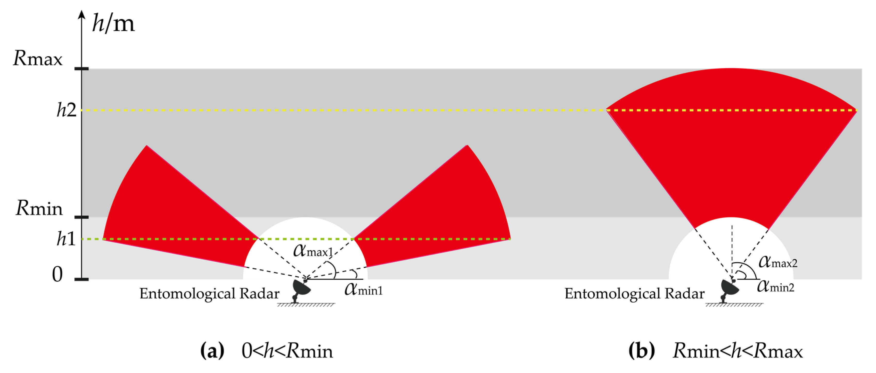
2.1. Fixed-Beam Vertical Looking Mode

In fixed-beam vertical-looking mode, the radar beam is adjusted vertical to the sky. The schematic diagram of this mode is shown in Figure 1.

To calculate the migration flux, the beam of the radar is divided into several equal height segments that are represented as $\mathsf{\Delta }h$ (Figure 1). The heights of the middle of each segment are represented as $\left(h_1,h_2,h_3,\dots h_k\dots \right)$, respectively. The minimum and maximum detection heights are denoted as $H_{\min }$ and $H_{\max }$, respectively. $R_{\min }$ and $R_{\max }$ denote the minimum and maximum radar detection ranges, respectively. For the vertical-looking mode, $H_{\min }=R_{\min }$, and $H_{\max }=R_{\max }$. The statistical time gap is defined as ∆T, and the sequence $\left(T_1,T_2,T_3,\dots T_n\dots \right)$ represents the middle time of each gap.

The number of insects detected by the radar in the k-th height layer and the n-th time gap is represented as $nu{m}_{k,n}$, and the minimum statistical unit is represented as (k, n). Assuming that the insect flies over the beam horizontally, the length of the detectable trajectory of the i-th target in the corresponding statistical unit is defined as $D_i(k,n)$. As migration flux represents the number of insects crossing the unit area per unit time, the contribution of one insect to the migration flux could be calculated as:

$$flu{x}^{\prime }(k,n)=\frac{1}{\mathsf{\Delta }{h}_k\mathsf{\Delta }{T}_n{D}_i(k,n)}$$

(1)

The migration flux is the sum of contributions of all insects:

$$\begin{array}{l}flux(k,n)={\displaystyle \sum _{i=1}^{nu{m}_{k,n}}flu{x}^{\prime }(k,n)}\\ =\frac{1}{\mathsf{\Delta }{h}_k\mathsf{\Delta }{T}_n}{\displaystyle \sum _{i=1}^{nu{m}_{k,n}}\frac{1}{D_i(k,n)}}\end{array}$$

(2)

Averaging over time, the mean migration flux can be expressed as:

$$Flux(k)=\frac{1}{N}\cdot {\displaystyle \sum _{n=1}^{N}flux(k,n)}$$

(3)

Equations (2) and (3) are the calculation method of insect migration flux under ideal conditions. In order to obtain the flux, $D_i(k,n)$ of all detected insects are required to be known. According to the description of Chapman J W et al. in the article [15], $D_i(k,n)$ is determined by the RCS of insects. For a radar without the capacity for in-beam angle measurement, the target RCS is measured based on the assumption that the insect crosses over the beam center. In the real situation, the probability of an insect crossing the beam center is extremely small. Therefore, the measured RCS is usually smaller than the real RCS ${\delta }_i$.

The three-dimensional radiation pattern of the antenna and its two-dimensional projection of a regular entomological radar are shown in Figure 2. When an insect crosses the beam at different positions, the amplitudes of the echo signals of the insect are shown in Figure 3.

As shown in Figure 3, the intensity of echo signals are different when the insect flies over the beam at different positions. The track B is closest to the LOS, and the radar receives the strongest echo power, hence the measured RCS is relatively large. The track A and C are far away from the LOS; therefore, the measured RCSs will be small.

As the measured insect RCS is usually less than the true value, the measured value of $D_i(k,n)$ is also smaller than the true value, which leads to the calculated value of migration flux $flux(k,n)$ being larger than the true value.

In order to solve this problem, this paper proposes a migration flux estimation method, based on statistical hypothesis. First of all, we will introduce how to calculate the measured length of the detectable trajectory of insect (denoted as $X_i(k,n)$), which depends on the measured RCS of the insect (usually smaller than the true value of RCS). When an insect crosses the radar beam, as shown in Figure 4, the radar measures L discrete trajectory points denoted as $A_l$ $(0<l\le L)$. From $A_0$ to $A_L$, the insect reflection signal amplitude varies from weak to strong and then weak. The point where the maximum target echo power occurs is denoted as $A_i$. The vector between the radar and point $A_i$ is defined as $\overrightarrow{O{A}_i}$, and $\left|\overrightarrow{O{A}_i}\right|=R_i$. Vector $\overrightarrow{OZ}$ represents LOS. The angle between vector $\overrightarrow{O{A}_i}$ and $\overrightarrow{OZ}$ is defined as ${\gamma }_i$. The vector from the radar to each trajectory point is $\overrightarrow{O{A}_l}$. The angle between $\overrightarrow{O{A}_i}$ and $\overrightarrow{O{A}_l}$ is defined as ${\theta }_l$. For a detected insect, the maximum of ${\theta }_l$ is ${\theta }_{\max }$.

The maximum detectable distance for an insect can be written as:

$$R_{\max \text{-}i}(k,n)={\left[\frac{C{G}^2(\theta ){\delta }_i(k,n)}{SN{R}_{min}}\right]}^{\frac{1}{4}}$$

(4)

where $C$ is the radar system gain coefficient, and it is determined by the entomological radar hardware [1,16]. ${\delta }_i(k,n)$ is the insect’s measured RCS in point $A_i$. $SN{R}_{\min }$ is the set minimum SNR for the detection threshold. $G(\theta )$ is the antenna gain pattern. Assuming that the radar’s antenna pattern is in Gaussian shape, which can be written as:

$$G(\theta )=\exp \left(\frac{-4\ln 2\cdot {\theta }_l{}^2}{{\theta }_{3db}^2}\right)$$

(5)

where ${\theta }_{3dB}$ is the half-power beamwidth of the antenna.

Taking Equation (5) into Equation (4), the maximum of ${\theta }_l$, i.e., the maximum detectable angle ${\theta }_{\max }$ can be calculated as [1]:

$${\theta }_{\max \text{-}i}(k,n)={\theta }_{3db}\sqrt{\frac{\ln \left(\frac{R_{\max \text{-}i}(k,n)}{R_i(k,n)}\right)}{2\ln 2}}$$

(6)

Then $X_i(k,n)$ can be approximated as:

$$X_i(k,n)\approx 2R_i(k,n)\cdot {\theta }_{\max \text{-}i}(k,n)$$

(7)

According to Equations (4)–(7), $X_i(k,n)$ can be obtained as:

$$X_i(k,n)\approx R_i(k,n)\cdot {\theta }_{3db}\sqrt{\frac{\ln \left[\frac{{\delta }_i(k,n)\cdot C}{R_i^4(k,n)SN{R}_{\min }}\right]}{2\ln 2}}$$

(8)

The ratio of $X_i(k,n)$ and $D_i(k,n)$ is defined as the deviation coefficient $\mu$:

$${\mu }_i(k,n)=\frac{X_i(k,n)}{D_i(k,n)}$$

(9)

Equation (2) can be also written as:

$$\begin{array}{ll}flux(k,n)& =\frac{1}{\mathsf{\Delta }{h}_k\mathsf{\Delta }{T}_n}{\displaystyle \sum _{i=1}^{nu{m}_{k,n}}\frac{1}{D_i(k,n)}}\\ & =\frac{1}{\mathsf{\Delta }{h}_k\mathsf{\Delta }{T}_n}nu{m}_{k,n}\mathrm{E}\left[\frac{1}{D_i(k,n)}\right]\\ & =\frac{nu{m}_{k,n}}{\mathsf{\Delta }{h}_k\mathsf{\Delta }{T}_n}\mathrm{E}\left[\frac{{\mu }_i(k,n)}{X_i(k,n)}\right]\end{array}$$

(10)

According to the previous discussion, in most cases ${\mu }_i(k,n)<1$. In the traditional calculation method, it assumes that the insect crosses the LOS, i.e., ${\mu }_i(k,n)=1$, which leads to the calculated flux being larger than the true value. As ${\mu }_i(k,n)$ is unknown, $flux(k,n)$ cannot be obtained based on Equation (10). To solve the problem, the following simplification is made:

$$\mathrm{E}\left[\frac{{\mu }_i(k,n)}{X_i(k,n)}\right]\approx \frac{\mathrm{E}\left[{\mu }_i(k,n)\right]}{\mathrm{E}\left[X_i(k,n)\right]}$$

(11)

Substituting (11) into (10) yields:

$$flux(k,n)\approx \frac{nu{m}_{k,n}}{\mathsf{\Delta }{h}_k\mathsf{\Delta }{T}_n}\frac{\mathrm{E}\left[{\mu }_i(k,n)\right]}{\mathrm{E}\left[X_i(k,n)\right]}$$

(12)

In (12), $\mathsf{\Delta }{h}_k$ and $\mathsf{\Delta }{T}_n$ are custom parameters; $\mathrm{E}\left[X_i(k,n)\right]$ and $nu{m}_{k,n}$ can be obtained from radar measurement. Only the expectation of the deviation coefficient $\mathrm{E}\left[{\mu }_i(k,n)\right]$ is unknown. To obtain $\mathrm{E}\left[{\mu }_i(k,n)\right]$, another hypothesis is made that the position of the insects in the air is uniformly distributed. As shown in Figure 5. when an insect crosses the beam, the distance between the trajectory and the LOS is defined as $Y_i(k,n)$.

According to the hypothesis, $Y_i(k,n)$ obeys a uniform distribution $\mathrm{U}\left[0,\frac{D_i(k,n)}{2}\right]$. Thereby, $\frac{Y_i(k,n)}{D_i(k,n)}$ obeys a uniform distribution $\mathrm{U}\left[0,\frac{1}{2}\right]$. $X_i(k,n)$ can be written as:

$$X_i(k,n)=\sqrt{D_i{}^2(k,n)-4Y_i{}^2(k,n)}$$

(13)

In (13), divide the two sides by $D_i(k,n)$ and calculate its expectation, and we get:

$$\mathrm{E}\left[\frac{X_i(k,n)}{D_i(k,n)}\right]=\mathrm{E}\left[\frac{1}{D_i(k,n)}\sqrt{D_i{}^2(k,n)-4Y_i{}^2(k,n)}\right]$$

(14)

(14) can be transformed as:

$$\mathrm{E}\left[{\mu }_i(k,n)\right]=\mathrm{E}\left[\sqrt{1-4{\left(\frac{Y_i(k,n)}{D_i(k,n)}\right)}^2}\right]$$

(15)

According to the definition of probability distribution function, $\mathrm{E}\left[{\mu }_i(k,n)\right]$ can be solved as:

$$\begin{array}{l}\mathrm{E}\left[{\mu }_i(k,n)\right]={\displaystyle {\int }_0^{\frac{1}{2}}2\sqrt{1-4{\left(\frac{Y_i(k,n)}{D_i(k,n)}\right)}^2}\mathrm{d}\frac{Y_i(k,n)}{D_i(k,n)}}\\ =\frac{1}{2}\arcsin (1)\approx 0.7854\end{array}$$

(16)

Substituting $\mathrm{E}\left[{\mu }_i(k,n)\right]$ into (12), we can obtain:

$$flux(k,n)\approx \frac{0.7854nu{m}_{k,n}}{\mathsf{\Delta }{h}_k\mathsf{\Delta }{T}_n\mathrm{E}\left[X_i(k,n)\right]}$$

(17)

2.2. Fixed-Beam Arbitrary Pointing Mode

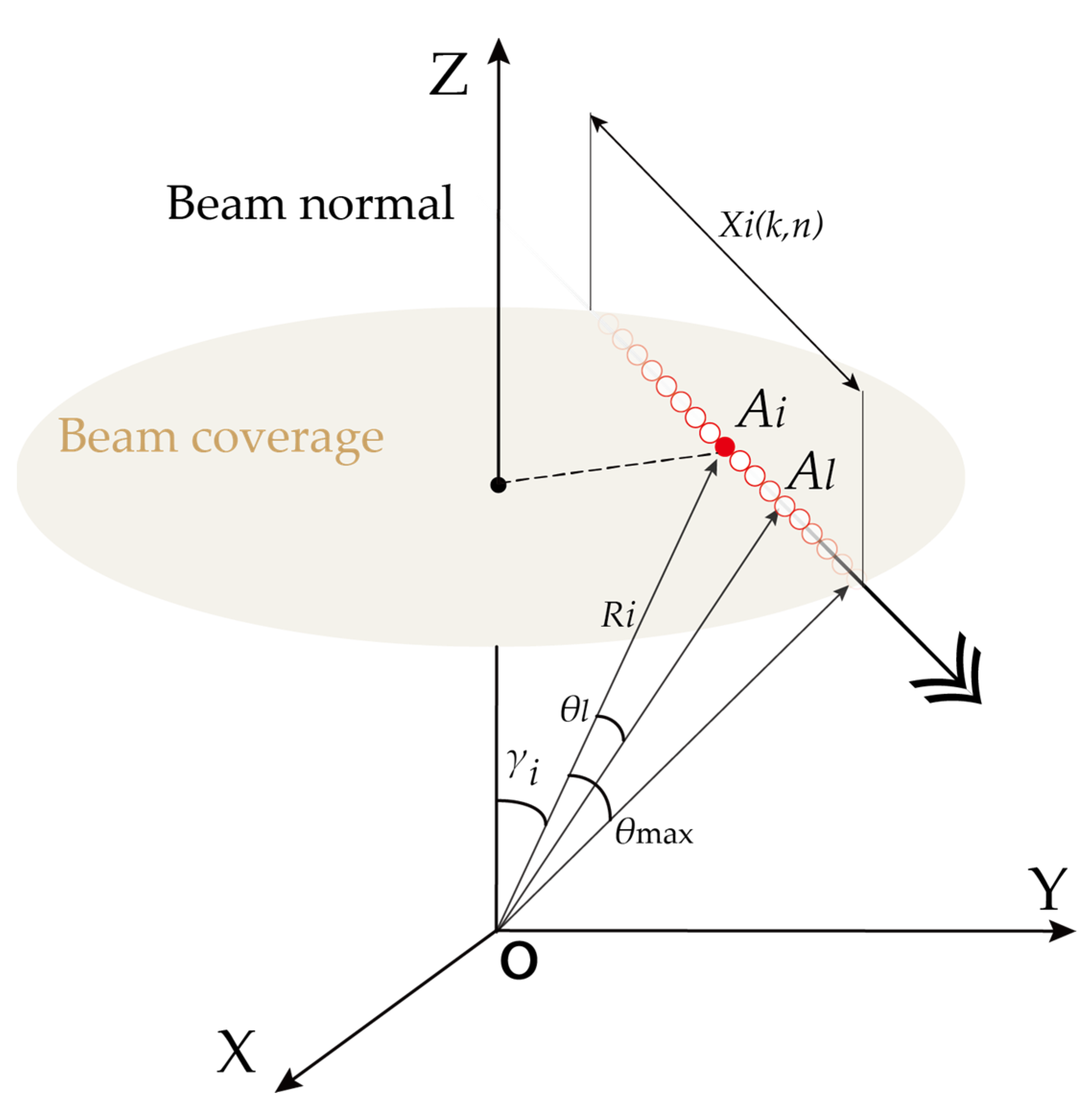
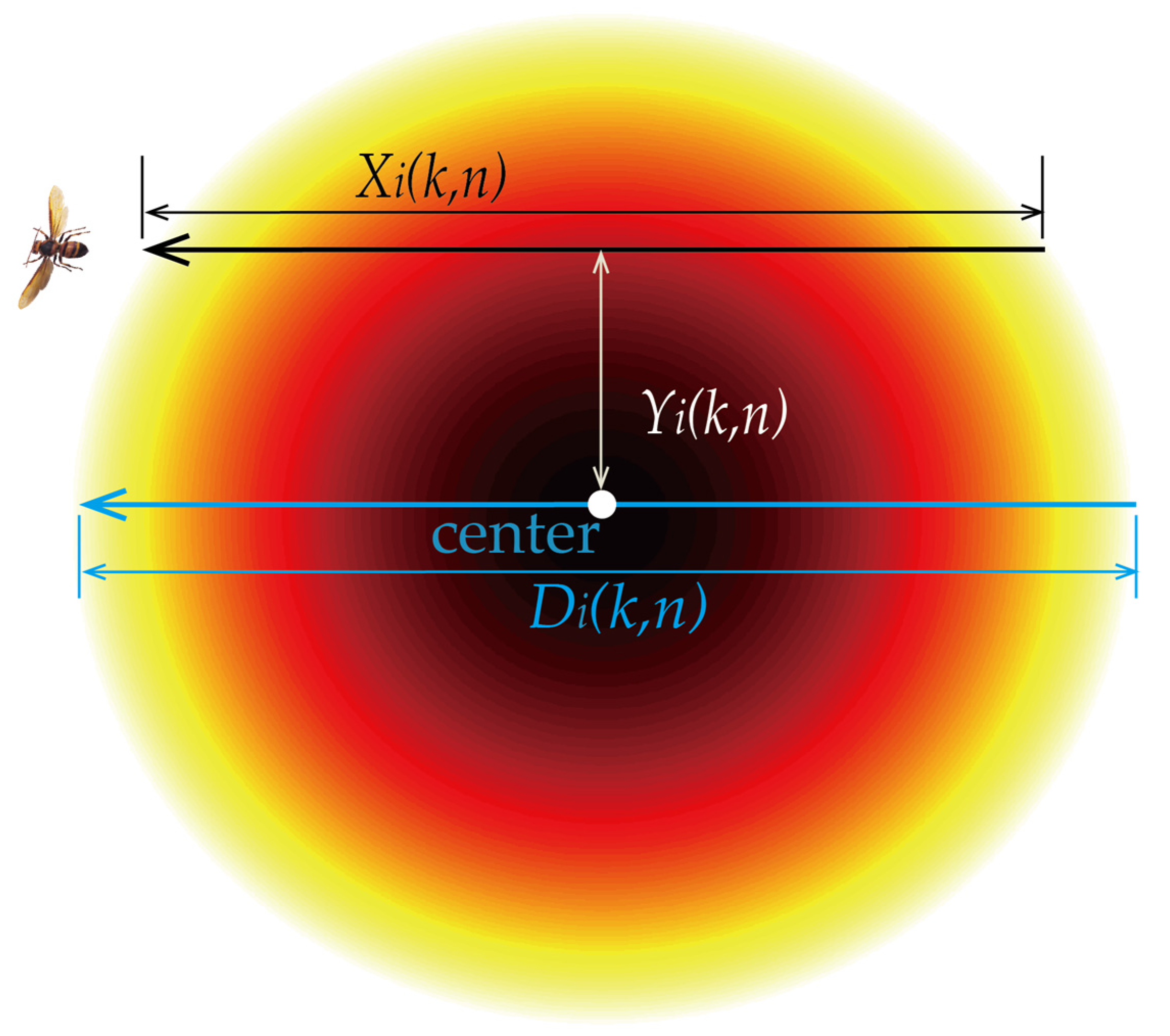
The previous subsection introduces the migration flux estimation method for fixed-beam vertical-looking mode. For more general cases, the entomological radar not only needs to measure the migratory situation directly above, but also needs to adjust the radar beam direction through the radar servo, so as to cover more airspace. This subsection presents the flux statistical model for fixed-beam arbitrary pointing mode.

As can be seen from Figure 6, when the entomological radar with a fixed beam is under an elevation of less than 90°, the range of the detectable height varies with the elevation $\alpha$. The relationship between the range of the detectable height and the detection range can be written as:

$$\{\begin{array}{l}{H}_{\min }=R_{\min }\sin \alpha \\ H_{\max }=R_{\max }\sin \alpha \end{array}$$

(18)

In order to simplify the calculation, the beam of the radar is still divided into several equal segments along the range dimension, as shown in the yellow area in Figure 6. The height of each segment can be calculated as $\mathsf{\Delta }h/\sin \alpha$. Similar to the vertical-looking mode, take the altitude of the center of the segment as the altitude of the segment.

Therefore, by replacing $\mathsf{\Delta }{h}_k$ with $\mathsf{\Delta }{h}_k/\sin \alpha$ of Equation (17), the migration flux $flux(k,n)$ for the fixed-beam arbitrary pointing mode can be obtained:

$$flux(k,n)\approx \frac{0.7854nu{m}_{k,n}\sin \alpha }{\mathsf{\Delta }{h}_k\mathsf{\Delta }{T}_n\mathrm{E}\left[X_i(k,n)\right]}$$

(19)

2.3. Scanning Mode

In order to monitor a wider airspace in the scanning mode, a new scanning mode for the entomological radar is proposed. The orientation and speed of the insects are needed. In this section, we describe the scanning parameters of the proposed scanning mode and the migration flux calculation method.

2.3.1. Scanning Mode Description

The migratory insects are expected to fly in a straight, steady line due to the need to maximize flight efficiency [3,11]. Most migratory insects can be covered when the radar beam scanning direction is perpendicular to the migrating direction. Therefore, to detect as many targets as possible, the azimuth angle of the radar could be set perpendicular to the migratory direction, and the beam is set to scan periodically in elevation. The scanning schematic is shown in Figure 7.

The azimuth and scanning speed are determined as follows. In order to maximize the coverage of migratory insects, the scanning direction of the radar is set vertical to the migratory direction. For example, if most of the insects migrate from the azimuth of ${23}^{°}$ north by east, the entomological radar azimuth should be set to ${113}^{°}$ north by east. The flying direction of the insects can be obtained in vertical-looking mode by measuring the orientation of the insects [17]. So, before working in the scanning mode, the radar should be set in vertical-looking mode for a while, to obtain a priori information of the migratory status.

The scanning speed is determined based on the tangential flight speed of the migratory insects, and the calculation method is described in detail in the article [17]. The tangential velocity sequence $\left(V_1,V_2,\dots ,V_i,\dots ,V_{Nu{m}_{k,n}}\right)$ and the height sequence $\left(h_1,h_2,\dots ,h_i,\dots h_{Nu{m}_{k,n}}\right)$ of the target are measured in the vertical-looking mode. The scanning angular velocity ${\omega }_{scan}$ can be set as the highest angular velocity of the target, relative to the radar, which is calculated as:

$${\omega }_{scan}=\max \left(\arctan \frac{V_i}{h_i}\right)$$

(20)

The purpose is to minimize the scanning period, and to avoid repeated detection of the target. It is noted that in (20), if ${\omega }_{scan}$ exceeds the maximum speed allowed by the servo hardware, ${\omega }_{scan}$ should be set to the maximum speed of the servo. At this point, the key parameters of the scanning mode are determined.

2.3.2. Flux Estimation Method for Scanning Mode

(1)

Statistical time gap

For the proposed scanning mode, the beam coverage time $\mathsf{\Delta }{T}_h$ at different heights is different. Now, we describe how to calculate the beam coverage time $\mathsf{\Delta }{T}_h$ at different heights during a scanning cycle. The scanning range in elevation of one scanning period is elevation from $0^{°}$ to ${180}^{°}$. Most entomological radars are pulsed radar systems, with non-zero $R_{\min }$. As shown in Figure 8, when the radar elevation is ${\mathsf{\alpha }}_1$, the detection height range is $\left[H_{\min 1},H_{\max 1}\right]$. When elevation is ${\alpha }_2$, the detection height range becomes $\left[H_{\min 2},H_{\max 2}\right]$, where $0\le {\alpha }_1<{\alpha }_2\le \frac{\pi }{2}$. It is easy to represent the two height ranges with the detection ranges as $\left[R_{\min }\sin {\alpha }_1,R_{\max }\sin {\alpha }_1\right]$ and $\left[R_{\min }\sin {\alpha }_2,R_{\max }\sin {\alpha }_2\right]$. Since $\sin {\alpha }_1<\sin {\alpha }_2$, for the larger elevation ${\alpha }_2$, the radar covers a larger altitude range.

It is assumed that the radar scans at a constant angular speed, and the acceleration and deceleration motion of the servo in the start–stop phase is ignored. The instantaneous beam coverage duration time $t_h$ is calculated as (21).

$$t_h=\frac{1}{{\omega }_{scan}}$$

(21)

In a scanning cycle, the beam scans at an elevation of $0$° to $180$° at a uniform angular speed. At height h, the beam coverage duration time is the sum of the instantaneous duration time of all elevations. As shown in Figure 9, the red area is the airspace that can be covered by the radar beam. As shown in Figure 9a, when $h_1\in \left[0,R_{\min }\right]$, the beam can cover height $h_1$ within the elevation range of $\left[{\alpha }_{\min 1},{\alpha }_{\max 1}\right]$ and $\left[{180}^{\circ }-{\alpha }_{\max 1},{180}^{\circ }-{\alpha }_{\min 1}\right]$. As shown in Figure 9b, when $h_2\in \left[R_{\min },R_{\max }\right]$, the beam can cover height $h_2$ within the elevation range of $\left[{\alpha }_{\min 2},{\alpha }_{\max 2}\right]$ and $\left[{180}^{\circ }-{\alpha }_{\max 2},{180}^{\circ }-{\alpha }_{\min 2}\right]$.

${\alpha }_{\min 1}$ and ${\alpha }_{\min 2}$ are determined by the current height h and $R_{\max }$. For example,${\alpha }_{\min 1}=\arcsin \frac{h_1}{R_{\max }}$, and ${\alpha }_{\min 2}=\arcsin \frac{h_2}{R_{\max }}$. Due to the radar blind range, when $h\in \left[0,R_{\min }\right]$ and $\alpha$ is higher than ${\alpha }_{\max 1}$, the height $h_1$ is out of detection coverage; thus, ${\alpha }_{\max 1}=\arcsin \frac{h_1}{R_{\min }}$. When $h\in \left[R_{\min },R_{\max }\right]$, the detectable height is not affected by the radar blind range; thus, ${\alpha }_{\max 2}=\frac{\pi }{2}$. The dwell time $\mathsf{\Delta }T(h)$ of the beam at height h is the integral of $t_h$ along $\alpha$:

$$\mathsf{\Delta }T(h)=\{\begin{array}{ll}2{\displaystyle {\int }_{arc\sin \frac{h}{R_{\max }}}^{arc\sin \frac{h}{R_{\min }}}{t}_{h}d\alpha }& ,(0\le h\le R_{\min })\\ 2{\displaystyle {\int }_{arc\sin \frac{h}{R_{\max }}}^{\frac{\pi }{2}}{t}_{h}d\alpha }& ,(R_{\min }\le h\le R_{\max })\end{array}$$

(22)

Taking (21) into (22), we can get:

$$\mathsf{\Delta }T(h)=\{\begin{array}{ll}\frac{2}{{\omega }_{scan}}\left(\arcsin \frac{h}{R_{\min }}-\arcsin \frac{h}{R_{\max }}\right)& ,(0\le h\le R_{\min })\\ \frac{2}{{\omega }_{scan}}\left(\frac{\pi }{2}-\arcsin \frac{h}{R_{\max }}\right)& ,(R_{\min }\le h\le R_{\max })\end{array}$$

(23)

The mapping diagram of h and $\mathsf{\Delta }T(h)$ is shown in Figure 10. The area with deeper color represents a longer beam coverage time. It can also be seen that the longest beam coverage time occurs at the height $R_{\min }$. Compared with the detection height range of the fixed beam looking mode, the scanning mode can cover the airspace with lower altitude.

(2)

Migration flux calculation

It is assumed that insect migration flux is consistent at the same altitude within the scanning range in one scanning period. The migration flux for scanning mode can be obtained by taking Equation (23) into Equation (19):

$$flux(k,n)=\{\begin{array}{ll}\frac{0.3927nu{m}_{k,n}{\omega }_{scan}\sin \alpha }{\mathsf{\Delta }{h}_k\left(\arcsin \frac{h}{R_{\min }}-\arcsin \frac{h}{R_{\max }}\right)\mathrm{E}\left[X_i(k,n)\right]}& ,(0\le h\le R_{\min })\\ \frac{0.3927nu{m}_{k,n}{\omega }_{scan}\sin \alpha }{\mathsf{\Delta }{h}_k\left(\frac{\pi }{2}-\arcsin \frac{h}{R_{\max }}\right)\mathrm{E}\left[X_i(k,n)\right]}& ,(R_{\min }\le h\le R_{\max })\end{array}$$

(24)

3. Results

3.1. Simulation Analysis

The insect migration flux estimation methods for three working modes are introduced above. The correctness and feasibility of the proposed methods are verified by the simulation and field test in this subsection. As the migration flux estimation methods for the fixed-beam arbitrary pointing mode and scanning mode are developed from the method proposed for fixed-beam vertical-looking mode, only the method proposed for fixed-beam vertical-looking mode is analyzed in this section.

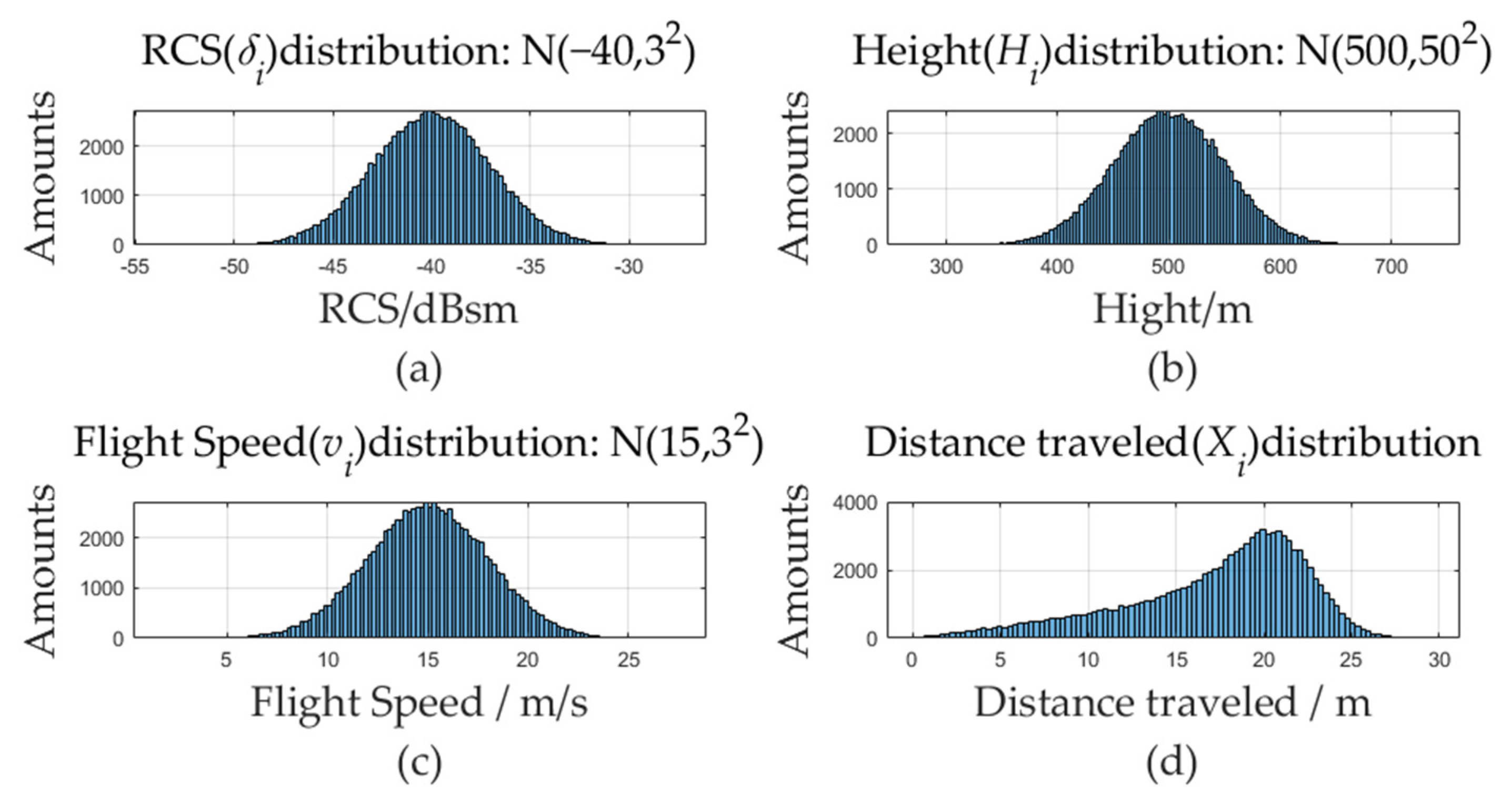
3.1.1. Method Simulation under Ideal Conditions

In this subsection, we simulate that, when the radar works in vertical-looking mode, ${10}^5$ migratory insects randomly cross the beam during 12 h. The migration flux is calculated according to the model designed in Section 2, and the results are compared with the theoretical values to verify the correctness and confidence range of the method.

The RCS ${\delta }_i$ of ${10}^5$ migratory insects are assumed to obey a normal distribution with the mean value $\mathrm{E}=$ −40 dBsm and standard deviation $\mathsf{\sigma }=3$ dBsm, as shown in Figure 11a. The migrating height $H_i$ obeys a normal distribution with mean value $\mathrm{E}=$ 500 m and standard deviation $\mathsf{\sigma }=$ 50 m, as shown in Figure 11b. The time $t_i$ of entry into the radar beam occurs randomly within 12 h. The migrating flight speed $v_i$ follows a normal distribution with mean value $\mathrm{E}$ of 15 m/s, and standard deviation $\mathsf{\sigma }$ of 3 m/s, as Figure 11c. The distance $Y_i$ from insect i to the center of the radar beam normal is assumed to obey a random uniform distribution $\mathrm{U}\left[0,\frac{D_i}{2}\right]$. According to the above assumptions, the deviation coefficient ${\mu }_i$ and the actual crossing distance $X_i$ could be solved, and the distribution of $X_i$ is shown in Figure 11d.

(1)

Theoretical migration flux results

According to the above assumptions of the simulation, the theoretical migration flux results could be calculated with the assumption that $\mathsf{\Delta }T=$ 60 s, and $\mathsf{\Delta }h=$ 5 m. Based on the ${\mu }_i$ and $X_i$, the longest crossing beam distance $D_i$ of each insect could be calculated by Equation (9). Then, the theoretical migration flux $flux(k,n)$ can be obtained based on Equation (2), the definition of migration flux, as shown in Figure 12a. Then, based on Equation (3), the average flux at different heights over 12 h is obtained, as shown in Figure 12b. These results are true values of insect migration flux for the simulation.

(2)

Migration flux calculated by the traditional method

For the traditional method, the actual cross beam position of insects is ignored, i.e., it is assumed that $D_i(k,n)\approx X_i(k,n)$. In each statistical unit (k,n), $flux(k,n)$ can be obtained, based on Equation (2), as shown in Figure 13a. Then, according to Equation (3), the height-average flux profile over 12 h is obtained, as shown in Figure 13b. It can be seen by comparison that the values of migration flux based on the traditional method are larger than the true values shown in Figure 12.

(3)

Migration flux by the proposed method

The migration flux results calculated based on the proposed method are shown in Figure 14a, where $\mathsf{\Delta }h=$ 5 m and $\mathsf{\Delta }T=$ 60 s. The height-average flux profile over 12 h is shown in Figure 14b. It can be seen that this result is close to the theoretical migration flux, shown in Figure 12.

In order to quantitatively evaluate the migration flux estimation accuracy, the flux-error-ratio $\eta$ is defined as:

$$\eta (k)=\left|\frac{Flu{x}_r(k)-Flu{x}_m(k)}{Flu{x}_r(k)}\right|$$

(25)

where $Flu{x}_r(k)$ and $Flu{x}_m(k)$ are the real flux and the measured flux at k-th height segment, respectively. According to the previous calculation results, the $\eta$ of the traditional flux calculation method and the proposed flux statistical method are recorded as ${\eta }_t$ and ${\eta }_n$. The comparison results are shown in Figure 15. ${\eta }_t$ is mostly concentrated between 0.2 and 0.4, which indicates that, if the positions of the insects passing through the beam are not considered, it will cause about 30% measurement error.

${\eta }_n$ is mostly less than 0.2. At a height of 400~600 m, where the number of insects is large, ${\eta }_n$ is even less than 0.025, which means that at this height segment, the migration flux measurement is very close to the real migration flux. The large number of insects at 400~600 m is caused by the assumption of the simulation that the insects are concentrated at 500 m, and obey the normal distribution. Therefore, the insects are mostly concentrated between 400~600 m, and there are relatively few insects in other height segments. The simulation results show that the larger the number of statistical samples, the smaller the error of the migration flux calculation results.

3.1.2. Influence of Number of Statistical Samples and RCS Measurement Error on Migration Flux Estimation

This subsection analyzes and simulates the influence of the number of statistical samples $nu{m}_{k,n}$ and the RCS measurement error on $\eta$ under the fixed-beam vertical-looking mode of entomological radar. In the natural environment, the statistical sample size is uncertain. In addition, the radar amplitude (RCS) measurement is generally with errors, due to the noise. This section simulates the change trend of $\eta$ when $nu{m}_{k,n}$ increases from 1 to 100 and the RCS measurement error increases from 0 to 5 dB. It can be seen from Equation (20) that ${\delta }_i$ affects the calculation results of $X_i(k,n)$, and from (15), that the error of $X_i(k,n)$ will lead to the calculation error of $flux(k,n)$. The simulation condition settings are shown in

Table 1. Simulation parameter table.

Number	Parameter Symbols	Parameter Value	Unit
1	${\delta }_i$	$\mathrm{N}(-40, 3^2)$	dBsm
2	$H_i$	$\mathrm{N}(500, {50}^2)$	m
3	$v_i$	$\mathrm{N}(15, 3^2)$	m/s
4	$Y_i$	$\mathrm{U}\left[0,\frac{D_i}{2}\right]$	-
5	Monte Carlo times	${10}^4$	-
6	Maximum error of amplitude measurement ${\xi }_{\max }$	$0, 0.5, 1 \dots 5$	dB
7	Amplitude measurement error $\xi$	$\mathrm{U}\left[-{\xi }_{\max },{\xi }_{\max }\right]$	dB
8	Statistical sample size $nu{m}_{k,n}$	1~100	-

$\mathrm{N}(\mu ,{\sigma }^2)$ denotes a normal distribution with mathematical expectation of $\mu$ and variance of ${\sigma }^2$. $\mathrm{U}\left[a,b\right]$ denotes a uniform distribution in section $\left[a,b\right]$.

:

It is assumed that the ${\delta }_i$, $H_i$ and $v_i$ of the target obey Gaussian distribution, and the random variable $Y_i$ obeys $\mathrm{U}\left[0,\frac{D_i}{2}\right]$ uniform distribution. The number of samples $nu{m}_{k,n}$ increases from 1 to 100 with an interval of 1. The amplitude measurement error $\xi$ increases from 0 to 5 dB, and $\xi$ is evenly distributed between $-{\xi }_{\max }$ and ${\xi }_{\max }$, which basically covers most of the performance indexes of entomological radar. The Monte Carlo simulation was conducted, and the $\eta$ with different sample numbers and amplitude errors are shown in Figure 16.

The simulation results show that $\eta$ increases with the increase of ${\xi }_{\max }$, and gradually decreases with the increase of the statistical sample size $nu{m}_{k,n}$. Under the condition of ${\xi }_{\max }\in \left[0,\hspace{0.17em}\hspace{0.17em}5\right] \mathrm{dB}$, when $nu{m}_{k,n}$ reaches 20, $\eta \in \left[0.053,\hspace{0.17em}\hspace{0.17em}0.073\right]$. When $nu{m}_{k,n}$ reaches 100, $\eta \in \left[0.025,\hspace{0.17em}\hspace{0.17em}0.068\right]$. According to the simulation results, in order to ensure that $\eta$ is low enough in application, $\mathsf{\Delta }h$ or $\mathsf{\Delta }T$ can be dynamically adjusting to realize the adaptive adjustment of $nu{m}_{k,n}$.

3.2. Experimental Verification

In this subsection, a Ku-band high-resolution fully polarimetric entomological radar developed by our team was used to verify the proposed migration flux estimation method. The radar was equipped with a two-dimensional servo. Through the rotation of the servo, the radar beam can be controlled to point to any direction in space. The azimuth rotation angle of the servo was 0°~360°, and the pitch coverage angle range was 0°~180° (the vertical pitch to the sky was $90$°) [18]. The radar adopted frequency modulation step-frequency technology to realize the broadband measurement, so that the radar had the characteristics of high range resolution [16,18]. By measuring the full polarization information of insects, the radar could obtain the orientation of insects.

The radar was set up in Jinyuan, Xundian, Kunming, Yunnan, China on 1 March 2021, and has been working all weather and all of the time. The radar installation site is an important migratory route for insects from Southeast Asia to China, Figure 17a is the radar scene picture, and Figure 17b is a satellite map of the radar installation location.

(1)

Verification results in fixed-beam vertical-looking mode

On 10 October 2021, the entomological radar worked in the fixed-beam vertical-looking mode. The detection height ranged from 150 m to 960 m. The insect migration flux was calculated with $\mathsf{\Delta }h=$ 25 m and $\mathsf{\Delta }T=$ 600 s, as shown in Figure 18.

Figure 18a shows the migration flux with different heights and times. It can be seen that there was a large-scale insect migration event that day. A large number of insects migrated at night (from early morning to 8:10 a.m., and from 5:10 p.m. to 12:00 p.m.), and a few insects migrated sporadically during the day. The peak of the whole day’s migration flux appeared at 6:50 a.m., and the peak flux reached $4.79\times {10}^{-3}$ $\mathrm{number}/{\mathrm{m}}^2/\mathrm{s}$. Figure 18b shows the height-average flux profile of the whole day. It can be seen that within the radar detection altitude range, the migration flux gradually increases with the decrease of altitude, and the maximum average flux in the whole day can reach $8.43\times {10}^{-4} \mathrm{number}/{\mathrm{m}}^2/\mathrm{s}$, which appeared near the height of 175 m from radar.

(2)

Verification results in fixed-beam arbitrary pointing mode

On 9 October 2021, the entomological radar worked in the fixed-beam arbitrary pointing mode, and the $\alpha$ was set to $75$°. The monitoring results of migration flux were statistically analyzed with $\mathsf{\Delta }h=$ 25 m and $\mathsf{\Delta }T=$ 600 s, and the monitoring height range was $\left[145,\hspace{0.17em}\hspace{0.17em}927\right]$ m. The results of 24-h insect migration flux are shown in Figure 19.

As can be seen from Figure 19a, the insect migration event on that day occurred from 6:30 a.m. to 7:20 a.m., and from 3:40 p.m. to 12:00 p.m. The peak of the migration flux appeared at 4:20 p.m., and the peak flux reached $5.9\times {10}^{-3} \mathrm{number}/{\mathrm{m}}^2/\mathrm{s}$. As can be seen from Figure 19b, within the radar detection altitude range, the migration flux gradually increased with the decrease of altitude, and the maximum average flux in the whole day reached $1.03\times {10}^{-3} \mathrm{number}/{\mathrm{m}}^2/\mathrm{s}$, which appeared near the height of 145 m from radar.

(3)

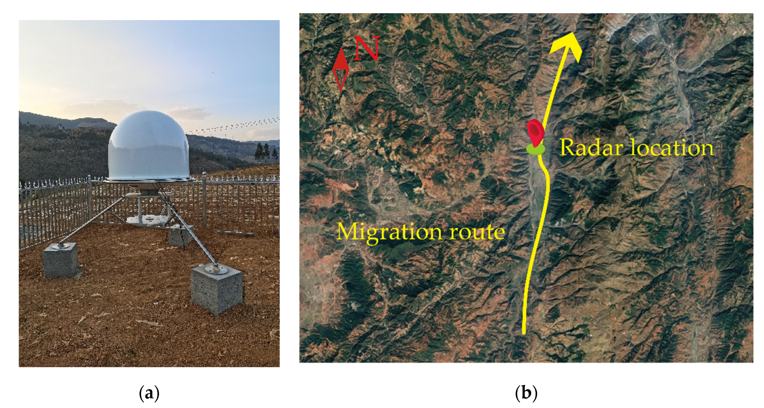
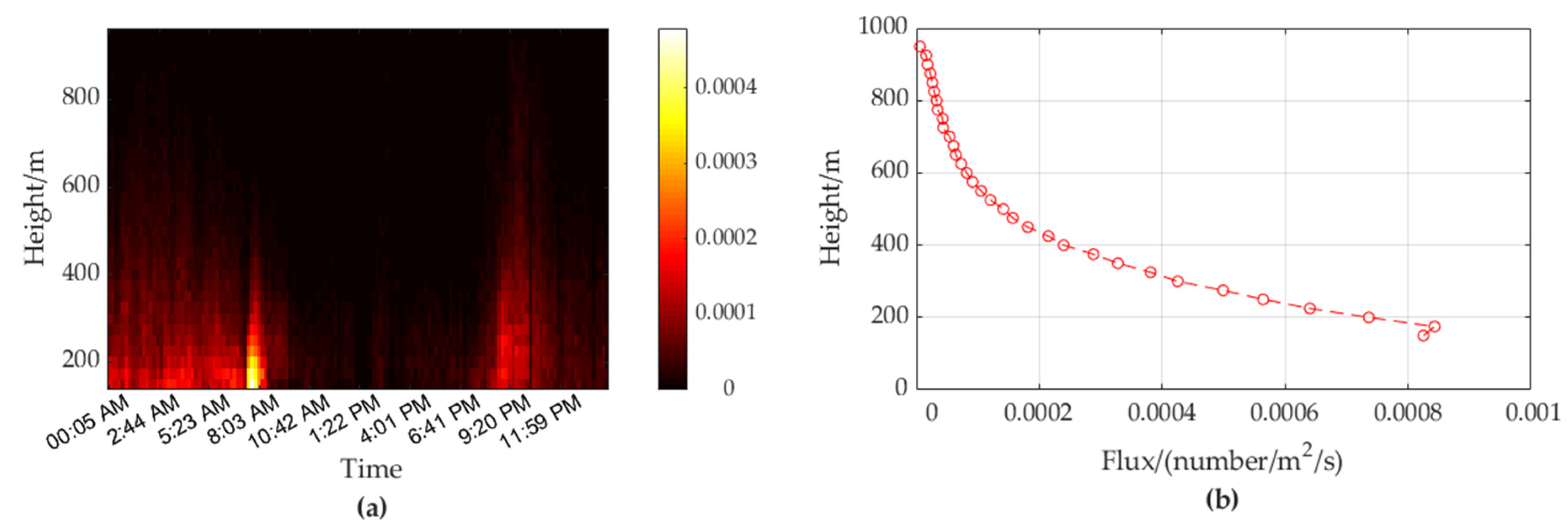
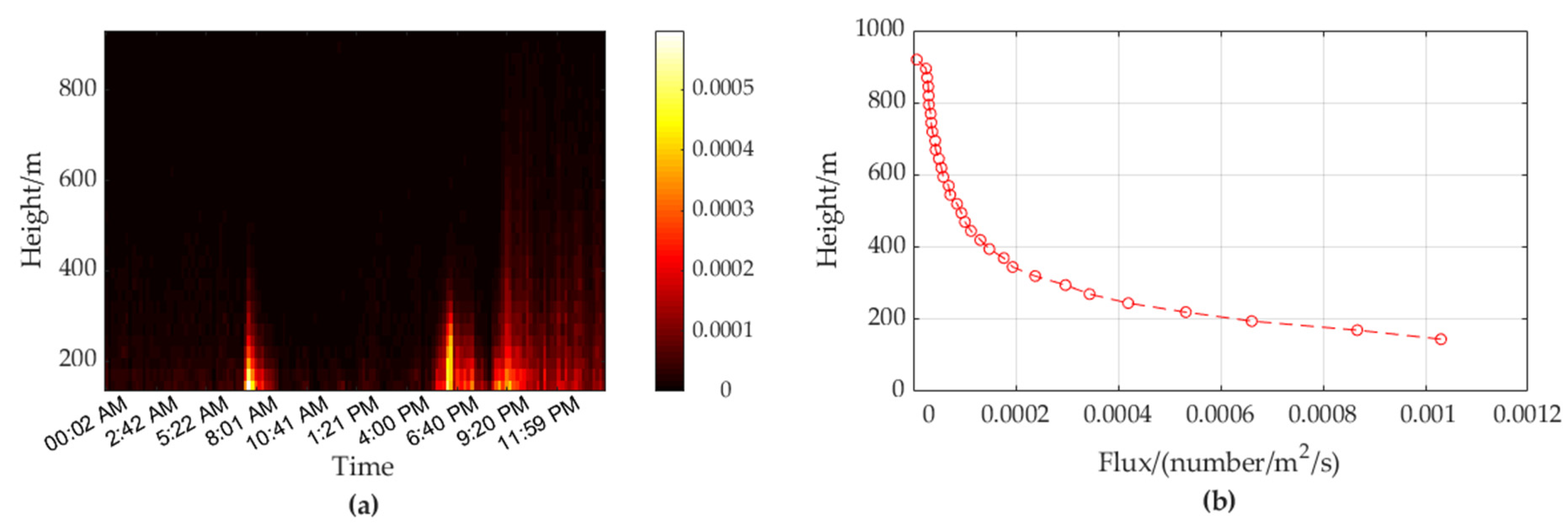
Verification results in scanning mode

On 29 October 2021, the entomological radar worked in the scanning mode. The monitoring results of migration flux were statistically analyzed with $\mathsf{\Delta }h=$ 25 m and $\mathsf{\Delta }T=$ 600 s, and the monitoring height range was $\left[0, 960\right]$ m. The results of the 24-h insect migration flux are shown in Figure 20.

As can be seen from Figure 20a, there was a migration event that day, which lasted from 6:30 a.m. to 6:20 p.m. After a short pause, it migrated again at 7:20 p.m. until 12 p.m. The peak of the whole day’s migration flux appeared at 4:50 p.m, and the peak flux reached $4.34\times {10}^{-3} \mathrm{number}/{\mathrm{m}}^2/\mathrm{s}$. As can be seen from Figure 20b, within the radar detection altitude range, the migration flux gradually increased with the decrease of altitude, and the maximum average flux in the whole day reached $1.1\times {10}^{-3} \mathrm{number}/{\mathrm{m}}^2/\mathrm{s}$, which appeared near 125 m height from radar.

4. Discussion

Since the accuracy of the statistical results of migration flux is related to the number of insects in the statistical unit, and the number of insects is unpredictable, the statistical height interval and time interval can be flexibly adjusted to obtain the statistical results with predictable accuracy.

For the scanning mode method designed in this paper, the pitch scanning angle is designed to be $0~180$°. However, the pitch scanning angle range of some scanning radars is only $0~90$°. In order to solve this problem, the elevation of a scanning cycle can be divided into two sections: $0~90$° and $90~180$°. In the section of $90~180$°, the same airspace coverage is obtained by increasing the azimuth angle by $180$° and scanning the elevation from $90$° to $0$°.

Another way to solve the influence of RCS measurement error on the statistical results of migration flux is to design an entomological radar with in-beam angle measurement function, which can measure the RCS of each insect more accurately. However, this method has higher requirements for hardware and greater complexity of the radar system.

In the fourth section, we introduced the field test results of insect migration flux. Limited by the lack of other verification methods, we can only confirm the rationality of the measurement results indirectly. In article [19], the statistical results of insect migration measured by Reynolds showed that, with the decrease of altitude, the number of insects first increased and then decreased, which is consistent with the results measured on 10 October 2021 and 29 October 2021 in this paper. In [19,20], the test results of T. Lewi and Reynolds showed that there was a peak in the migration number of insects at sunrise and after sunset, which is also consistent with the results measured on 10 October 2021 and 9 October 2021 (the sunrise and sunset time are 7:10 a.m. and 6:55 p.m., respectively, at the radar site) in this paper. Therefore, it is reasonable to believe that the field test results of this paper are correct.

5. Conclusions

In this paper, an estimation method for migration flux is proposed for entomological radar without the capacity for addition in-beam angle measurement. The method can solve the problem of large estimation error of migration flux caused by RCS measurement errors when insects do not pass through the central beam. The migration flux estimation method for the fixed-beam vertical-looking mode is developed, and its extended application for the fixed-beam arbitrary pointing mode and a new proposed scanning mode are introduced. The effectiveness of the proposed method is verified based on simulation. Compared with the traditional method, the proposed method can greatly improve the accuracy of the estimation of migration flux for entomological radar, without the capacity for in-beam angle measurement. The influence of the number of statistical samples and RCS measurement error on the proposed method is analyzed by simulation. A large number of insect samples and a small RCS measurement error can improve the estimation accuracy of the proposed method. In addition, by using a Ku-band high-resolution fully polarimetric entomological radar set up in the outfield, the effectiveness of the proposed method is verified based on the measured data.

References

1. Chapman, J.; Smith, A.; Woiwod, I.; Reynolds, D.; Riley, J. Development of vertical-looking radar technology for monitoring insect migration. Comput. Electron. Agric. 2002, 35, 95–110. [Google Scholar] [CrossRef]
2. Cai, J.; Yuan, Q.; Wang, R.; Liu, C.; Zhang, T. Insect detection and density estimation based on a Ku-band scanning entomological radar. J. Eng. 2019, 2019, 7636–7639. [Google Scholar] [CrossRef]
3. Zhai, B.P. Entomological Radar: From Research to Practice. J. Remote Sens. 2001, 5, 240. [Google Scholar]
4. Cheng, D.F.; Wu, K.M.; Tian, Z.; Wen, L.P.; Shen, Z.R. Acquisition and analysis of migration data from the digitised display of a scanning entomological radar. Comput. Electron. Agric. 2002, 35, 63–75. [Google Scholar] [CrossRef]
5. Drake, V.A. Quantitative Observation and Analysis Procedures for a Manually Operated Entomological Radar; CSIRO: Melbourne, Australia, 1981. [Google Scholar]
6. Hu, C.; Kong, S.; Wang, R.; Zhang, F.; Wang, L. Insect Mass Estimation Based on Radar Cross Section Parameters and Support Vector Regression Algorithm. Remote Sens. 2020, 12, 1903. [Google Scholar] [CrossRef]
7. Long, T.; Hu, C.; Wang, R.; Zhang, T.; Zeng, T. Entomological radar overview: System and signal processing. IEEE Aerosp. Electron. Syst. Mag. 2020, 35, 20–32. [Google Scholar] [CrossRef]
8. Hu, C.; Kong, S.; Wang, R.; Long, T.; Fu, X. Identification of Migratory Insects from their Physical Features using a Decision-Tree Support Vector Machine and its Application to Radar Entomology. Sci. Rep. 2018, 8, 5449. [Google Scholar] [CrossRef] [Green Version]
9. Wang, R.; Mao, H.; Hu, C.; Zeng, T.; Long, T. Joint association and registration in a multiradar system for migratory insect track observation. IEEE Trans. Aerosp. Electron. Syst. 2021, 57, 4028–4043. [Google Scholar] [CrossRef]
10. Yu, T.; Li, M.; Li, W.; Mao, H.; Wang, R.; Hu, C.; Long, T. Polarimetric Calibration Technique for a Fully Polarimetric Entomological Radar Based on Antenna Rotation. Remote Sens. 2022, 14, 1551. [Google Scholar] [CrossRef]
11. Hu, C.; Li, W.; Wang, R.; Li, Y.; Li, W.; Zhang, T. Insect flight speed estimation analysis based on a full-polarization radar. Sci. China Inf. Sci. 2018, 61, 1–3. [Google Scholar] [CrossRef] [Green Version]
12. Hu, C.; Kong, S.; Wang, R.; Zhang, F. Radar Measurements of Morphological Parameters and Species Identification Analysis of Migratory Insects. Remote Sens. 2019, 11, 1977. [Google Scholar] [CrossRef] [Green Version]
13. Chao, Z.; Rui, W.; Hu, C. Equivalent point estimation for small target groups tracking based on MLE. Sci. China Inf. Sci. 2019, 63, 8. [Google Scholar]
14. Li, W.; Hu, C.; Wang, R.; Kong, S.; Zhang, F. Comprehensive analysis of polarimetric radar cross-section parameters for insect body width and length estimation. Sci. China Inf. Sci. 2021, 64, 11. [Google Scholar] [CrossRef]
15. Chapman, J.W.; Reynolds, D.R.; Smith, A.D. Vertical-Looking Radar: A New Tool for Monitoring High-Altitude Insect Migration. BioScience 2003, 53, 503–511. [Google Scholar] [CrossRef] [Green Version]
16. Yu, T.; Wang, R.; Li, M.; Hu, C. Research on the design and calibration of wideband fully polarized vertical insect radar. J. Signal Process. 2021, 37, 222–233. [Google Scholar]
17. Wang, R.; Li, W.; Hu, C.; Li, M.; Mao, H. Insect Biological Parameters Estimation Method and Field Quantitative Experiment Verification for Fully Polarimetric Entomological Radar. J. Signal Process. 2021, 37, 199–208. [Google Scholar]
18. Wang, R.; Cai, J.; Hu, C.; Zhou, C.; Zhang, T. A Novel Radar Detection Method for Sensing Tiny and Maneuvering Insect Migrants. Remote Sens. 2020, 12, 3238. [Google Scholar] [CrossRef]
19. Reynolds, D.R.; Smith, A.D.; Chapman, J.W. A radar study of emigratory flight and layer formation by insects at dawn over southern Britain. Bull. Entomol. Res. 2008, 98, 35–52. [Google Scholar] [CrossRef] [PubMed]
20. Lewis, T.; Taylor, L.R. Diurnal periodicity of flight by insects. Trans. R. Entomol. Soc. Lond. 1965, 116, 393–435. [Google Scholar] [CrossRef]
Figure 1. Schematic diagram of radar beam in fixed-beam vertical-looking mode.
Remotesensing 14 02298 g001
Figure 2. Projection of entomological radar spatial radiation intensity.
Remotesensing 14 02298 g002
Figure 3. Schematic diagram of amplitudes of echo signal of an insect crossing the beam at different positions.
Remotesensing 14 02298 g003
Figure 4. Schematic diagram of insects crossing beam discrete points.
Remotesensing 14 02298 g004
Figure 5. Deviation coefficient μ schematic definition.
Remotesensing 14 02298 g005
Figure 6. Schematic diagram of fixed-beam arbitrary pointing mode.
Remotesensing 14 02298 g006
Figure 7. Schematic diagram of the proposed scanning mode.
Remotesensing 14 02298 g007
Figure 8. Differences in coverage height range at different elevations. (a) Radar beam coverage height at low elevation α 1 ; (b) Radar beam coverage height at high elevation α 2 .
Remotesensing 14 02298 g008
Figure 9. Schematic diagram of beam coverage time range corresponding to height h. (a) h [ 0 , R min ] ; (b) h [ R min , R max ] .
Remotesensing 14 02298 g009
Figure 10. Schematic diagram of relationship between coverage time and height in scanning mode.
Remotesensing 14 02298 g010
Figure 11. Assumptions of simulation. (a) RCS δ i distribution; (b) Height H i distribution; (c) Speed v i distribution; (d) Actual crossing distance X i distribution.
Remotesensing 14 02298 g011
Figure 12. Theoretical insect migration flux. (a) Migration flux with height-interval Δ h = 5 m, and time-interval Δ T = 60 s; (b) Height-average flux profile over 12 h.
Remotesensing 14 02298 g012
Figure 13. Insect migration flux results based on traditional method. (a) Migration flux with height-interval Δ h = 5 m, and time-interval Δ T = 60 s; (b) Height-average flux profile over 12 h.
Remotesensing 14 02298 g013
Figure 14. Insect migration flux results based on the proposed statistical method. (a) Migration flux with height-interval Δ h = 5 m, and time-interval Δ T = 60 s; (b) Height- average flux profile over 12 h.
Remotesensing 14 02298 g014
Figure 15. Flux error ratios η of the traditional and proposed method.
Remotesensing 14 02298 g015
Figure 16. Influence of amplitude measurement error and statistical sample number on η .
Remotesensing 14 02298 g016
Figure 17. Ku-band high-resolution fully polarized entomological radar. (a) Radar scene picture; (b) Satellite map of radar installation location.
Remotesensing 14 02298 g017
Figure 18. Migration flux measured under fixed-beam vertical-looking mode. (a) Migration flux with height-interval Δ h = 25 m, and time-interval Δ T = 600 s; (b) Height-average flux profile.
Remotesensing 14 02298 g018
Figure 19. Migration flux measured under fixed-beam arbitrary pointing mode. (a) Migration flux with height-interval Δ h = 25 m, and time-interval Δ T = 600 s; (b) Height-average flux profile.
Remotesensing 14 02298 g019
Figure 20. Migration flux measured under scanning mode. (a) Migration flux with height-interval Δ h = 25 m, and time-interval Δ T = 600 s; (b) Height-average flux profile.
Remotesensing 14 02298 g020