Integrating Hybrid Pyramid Feature Fusion and Coordinate Attention for Effective Small Sample Hyperspectral Image Classification

Abstract

In recent years, hyperspectral image (HSI) classification (HSIC) methods that use deep learning have proved to be effective. In particular, the utilization of convolutional neural networks (CNNs) has proved to be highly effective. However, some key issues need to be addressed when classifying hyperspectral images (HSIs), such as small samples, which can influence the generalization ability of the CNNs and the HSIC results. To address this problem, we present a new network that integrates hybrid pyramid feature fusion and coordinate attention for enhancing small sample HSI classification results. The innovative nature of this paper lies in three main areas. Firstly, a baseline network is designed. This is a simple hybrid 3D-2D CNN. Using this baseline network, more robust spectral-spatial feature information can be obtained from the HSI. Secondly, a hybrid pyramid feature fusion mechanism is used, meaning that the feature maps of different levels and scales can be effectively fused to enhance the feature extracted by the model. Finally, coordinate attention mechanisms are utilized in the network, which can not only adaptively capture the information of the spectral dimension, but also include the direction-aware and position sensitive information. By doing this, the proposed CNN structure can extract more useful HSI features and effectively be generalized to test samples. The proposed method was shown to obtain better results than several existing methods by experimenting on three public HSI datasets.

1. Introduction

Images with high spectral dimension and high spatial resolution are called hyperspectral images (HSIs) [1]. They can characterize the physical, chemical and material properties of objects. Due to its characteristics, people use HSI to solve problems in a variety of real situations, such as in precision agriculture [2,3,4], the military industry [5,6,7] and environmental monitoring [8,9,10]. Assigning a category to each pixel in the HSI is a HSIC task. This task is also a basic task in HSI processing [11].

In previous works of HSI classification tasks, due to the rich spectral feature information of hyperspectral images, traditional machine learning algorithms employ spectral information to solve HSIC tasks. This involves the use of support vector machines (SVMs) [12], Bayesian models [13], k-nearest neighbor (KNN) [14], etc. Nevertheless, these methods have common drawbacks, such as always using only spectral information for computing to assign a class to each pixel. In these methods, ignoring spatial information may lead to misclassification of pixels to a certain extent. Therefore, researchers have proposed many methods to exploit spectral feature information and spatial feature information to strengthen the presentation of hyperspectral images and raise the accuracy of classification [15,16,17,18,19,20,21]. For example, Markov random field [17], sparse representation [18], metric learning [15] and compound kernels [16,21]. In hyperspectral images, spectral information is always redundant, and spectral information belongs to a certain type of pixel, which is likely to be mixed with other types of information of HSI pixels. Therefore, in HSI classification, these methods are not effective in extracting discriminative but robust information. However, the classification effect is not always good. To address the spectral redundancy problem, some dimensionality reduction techniques focus on extracting effective features, as well as, for example, the widely used principal component analysis (PCA) [22], independent component analysis (ICA) [23] and factor analysis (FA) methods [24].

Recently, HSIC methods that using deep learning have proved to be effective [25,26,27,28]. Such methods include stacked autoencoder (SAE), deep belief network (DBN) and convolutional neural network (CNN). Chen et al. [29] first used SAE in HSIC. This method, combined with transfer learning, proposed a new model to fuse spectral-spatial features to obtain higher classification accuracy. Similarly, Li et al. [30] presented a model to capture spectral-spatial features for HSIC using a multilayer DBN. To alleviate the neglect of spatial information by the above methods, methods have been introduced that use CNN to solve HSI classification tasks [31]. CNN can make good use of the spatial relationships between images, which is popular in HSIC. Chen et al. [32] only used 3D-CNN to capture spectral-spatial information to classify HSIs, but the network model is simple and has limited effect. Therefore, Roy et al. [33] presented a hybrid 3D-2D CNN network that can obtain spectral-spatial feature information more efficiently. Zhong et al. [34] proposed a model named spectral-spatial residual network (SSRN). It can promote back-propagation of gradients while capturing richer spectral features and improving the performance of the model. Gao et al. [35] proposed a spectral feature enhancement-based sandwich CNN (SFE-SCNN), which can obtain better prediction results by enhancing the spectral features. Hang et al. [36] introduced a multi-task generative adversarial network (MTGAN) to classify HSIs using the rich information of unlabeled samples.

Although the above methods can enhance the classification effect of HSI with small sample training, they are still unsatisfactory. In recent years, to further improve classification performance, attention mechanisms have been extensively employed [37,38]. Researchers have utilized attention mechanisms in HSIC [39], which is also the most recent mainstream HSI classification method. Mei et al. [40] used a spectral-spatial network with attention mechanism and achieved good results. Recently, Zhu et al. [41] introduced residual spectral-spatial attention network (RSSAN) by introducing a spectral-spatial attention layer to SSRN. Mou et al. [42] proposed a block network called the spectral attention block, and used a gating mechanism for enhancing the spectral information in HSIC. Ray et al. [43] proposed A²S²K-ResNet, which could fully acquire the spectral-spatial features in the HSI cube by using residual 3D convolution, and inserted an attention block to weight the spectral-spatial features. Wu et al. [44] employed a two-branch spectral-spatial attention structure to classify HSI, where the two branches of the network focus on extracting spectral-spatial information, respectively. Although the above-mentioned attention-based methods for small sample HSI classification have achieved competitive classification performance, they still do not utilize the spectral-spatial feature information at different levels and scales, or the direction-aware and position sensitive information of hyperspectral images, which will have an impact on the classification to some extent.

In this paper, a new network that integrates hybrid pyramid feature fusion and coordinate attention is proposed to solve HSIC tasks under small sample training condition. Firstly, a baseline network is constructed, which is hybrid 3D-2D CNN. Compared with using 3D CNN or 2D CNN alone, using a hybrid 3D-2D CNN can obtain more useful HSI features. Secondly, three parallel hybrid 3D-2D CNNs are constructed. Using the hybrid pyramid feature fusion technology, the spatial information, detail information of different levels and scales can be fused to effectively complement each other and strengthen the performance of the model. Finally, the model utilizes a coordinate attention mechanism, which can not only capture spectral information, but also position sensitive and direction-aware features and enable the model to locate and identify target regions more accurately.

The innovative nature of this paper lies in three main areas:

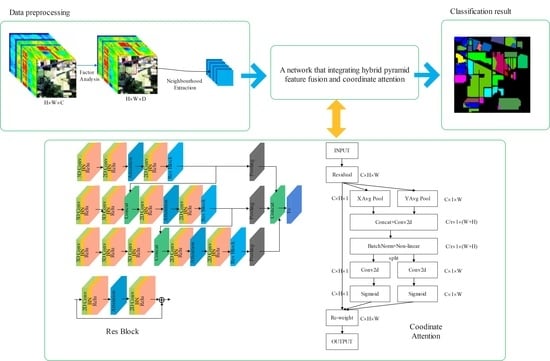
• A network that integrates hybrid pyramid feature fusion and coordinate attention is introduced for HSIC under small sample training conditions. This model can extract more robust spectral-spatial feature information during training small samples and has better classification performance than several other advanced models;
• A hybrid pyramid feature fusion is proposed, which can fuse the feature information of different levels and scales, effectively enhancing the spectral-spatial feature information and enhancing the performance of the small sample HSIC result;
• A coordinate attention mechanism is introduced for HSIC, which can not only weight spectral dimensions, but also capture position sensitive and direction-aware features in hyperspectral images, in order to enhance feature information extracted from small sample training.

2. The Proposed Method

In this section we describe the proposed method explicitly, including the data preprocessing, hybrid pyramid feature fusion network, coordinate attention mechanism, residual attention module and loss function.

2.1. The Framework of Proposed Model

Figure 1 is the overall framework of the proposed model. Firstly, we reduce the dimension of the HSI cube via Factor Analysis (FA) and then extract the overlapping 3D patches from the dimension reduced HSI cube as the input data. Each patch is extracted around a center pixel and the class of 3D patch is the class of the central pixel. Secondly, the proposed network model is composed of three parallel hybrid 3D-2D CNNs and a coordinate attention mechanism combined with a hybrid pyramid feature fusion mechanism. These three parallel networks are pooled through global average pooling and the three feature maps are fused. Finally, the features generated in the previous steps are classified through the FC layer to obtain the prediction results. Next, each of the principal steps of the proposed method are explicitly described.

2.1.1. Data Preprocessing

The input HSI cube is defined as $I\in R^{H\times W\times C}$, the initial input image is $I$, the width is $H$, the height is $W$ and the spectral dimension is $C$. The processes of data preprocessing are described as follows.

Firstly, the dimension of the HSI cube is reduced as $P\in R^{H\times W\times D}$ by Factor Analysis (FA), where $P$ is the processed input via FA, the number of spectral bands is $D$. This dimension reducing process can decrease the training time by 60% [45]. Using FA as a pre-processing step in HSIC task is very beneficial because FA can describe the variability between different correlated and overlapping spectral bands which helps the model to better classify similar examples. On the other hand, commonly used Principal Component Analysis (PCA) based reductions do not directly address this goal in HSI classification. PCA provides an approximation of the required factors, which does not help distinguish similar examples well. After the FA step, we extracted the 3D patches $X\in R^{S\times S\times D}$ from $P$, centered at pixel point $(\alpha ,\beta )$, covering the spatial size of $S\times S$ and the full spectral dimension D. We can calculate the number of 3D patches from $(H-S+1)\times (W-S+1)$. Therefore, the 3D patch at pixel point $(\alpha ,\beta )$, defined by $X_{(\alpha ,\beta )}$, selects the height from $\beta -(S-1)/2$ to $\beta +(S-1)/2$, the width from $\alpha -(S-1)/2$ to $\alpha +(S-1)/2$ and all $D$ spectral dimensions of $P$. Overlapping 3D patches of size $S\times S\times D$ are extracted from the preprocessed HSI and input into the proposed model. $S\times S$ is the sliding window size for patch extraction. The 3D patch size has been set to $15\times 15\times 30$ for the Indian Pines dataset, $19\times 19\times 20$ and $19\times 19\times 30$ for the University of Pavia and Salinas scene datasets, respectively. The size of 3D patch is chosen experimentally to maximize overall accuracy. The ground-truth of these patches is determined by the class category of the center pixel.

2.1.2. Hybrid Pyramid Feature Fusion Network

The hybrid pyramid feature fusion network consists of three parallel hybrid 3D-2D CNNs combined with a hybrid pyramid feature fusion. The network architecture can be seen in Figure 2. Firstly, we present the hybrid 3D-2D CNN, the network structure is shown in Part 1 of Figure 2. A 3D convolutional layer is employed to obtain spectral-spatial feature information. The first 2D convolution is used for dimensionality reduction, which can reduce the amount of computation and model complexity; the second 2D convolution is used to acquire further abstract spatial feature information. Using Res Block can increase the network depth, which extracts high-level semantic feature information. It also mitigates to some extent the problem of gradient explosion and gradient disappearance. The Res Block architecture is shown in Figure 3. Inputting the features generated in the previous step into the global average pooling can aggregate the feature information. Using the global average pooling can enhance computing speed and avoid overfitting. Finally, the feature maps from the global average pooling are passed to the FC layer for classification. The hybrid 3D-2D CNN can sufficiently leverage spectral and spatial feature information, reduce the complexity of the model, prevent overfitting and obtain better prediction results.

However, the HSI cube exhibits the phenomenon that “the same spectral dimensions may represent different categories and the same categories may represent different spectral dimensions”. The use of a single level and single scale feature does not reflect well the characteristic information of the HSI. Therefore, this paper adds a hybrid pyramid feature fusion mechanism to the above-mentioned hybrid 3D-2D CNN basic structure. This mechanism is useful for obtaining enriched features under small sample training conditions. The hybrid pyramid feature fusion network architecture is shown in Figure 2. The three parallel hybrid 3D-2D CNN structures have different numbers of 3D convolution layers, which are 1, 2, and 3, respectively. Designing the network structure in this way can extract spectral-spatial feature information with different scales. This hybrid pyramid feature fusion method fuses feature maps in two ways. The first method of feature fusion is to fuse features between different levels. Fusion of the feature map output by the Res Block in Part 1 and the feature map output by the 3D convolution layer in Part 2, and the fusion method of Part 2 and Part 3 is the same. The second method of feature fusion is to perform feature fusion between different scales. Res Block’s feature maps at different scales output in three parallel 3D-2D hybrid CNNs were fused after global average pooling aggregation. This design takes full advantage of the strong complementarity and correlation information of the feature with different levels, effectively fuses the information of the feature at different scales, obtains the deeper feature of the network during small sample training, and avoids overfitting. It can effectively improve network generalized ability.

2.1.3. Coordinate Attention Mechanism

Attention mechanisms that tell models “what to pay attention to” and “where to pay attention to” have been extensively studied [38,46] and are widely used to enhance the performance of models [37,47,48,49,50,51]. Attention mechanism [37] is inspired from the way the human eye observes things because the human eye always concentrates on the most important aspects of things. Likewise, it allows the network to dedicate itself to the important feature, which is helpful to the accuracy of the network [52]. In the HSIC task, the accuracy of the classification will be further enhanced by applying the attention mechanism to the network model. The essence of the attention mechanism is to weight the feature maps so that the model can focus on the important feature information and improve the model generalized ability. Figure 4 shows two typical attention mechanism structures.

SE attention and CBAM are the current most popular attention mechanisms. SE attention uses 2D global pooling to calculate channel attention weights and weight the feature information to optimize the model. The structure is shown as Figure 4a. However, SE attention weights the channel dimension of the feature map, but neglects the spatial dimension, which is crucial in computer vision tasks [53]. CBAM uses channel pooling and convolution to weight spatial dimension, as shown in Figure 4b. However, convolution cannot capture the relevance of long range information, which is critical to the vision task [51,54].

Therefore, the coordinate attention mechanism [55] is proposed, as shown in Figure 5. The coordinate attention mechanism can obtain the cross spectral, position sensitive and direction aware information. It assists the model to concentrate useful feature information. Global average pooling (GAP) is usually used to calculate channel attention weights and to globally encode spatial information, and GAP is performed for every spectral feature on the spatial dimension $H\times W$, the squeeze step $y$ is denoted as follows:

$$y=\frac{1}{H\times W}{\displaystyle \sum _{\alpha =1}^H{\displaystyle \sum _{\beta =1}^{W}x(\alpha ,\beta )}},$$

(1)

where $x(\alpha ,\beta )$ is denoted as the value of $x$ at position $(\alpha ,\beta )$.

However, it calculates channel attention weights by compressing the global spatial information so that there is a loss of spatial information. Therefore, the 2D global pooling is decomposed into 1D global pooling in the horizontal and vertical directions to effectively use both spatial and spectral information. Specifically, encoding of each spectral dimension in a feature map with spatial extent in $(H,1)$ and $(1,W)$ occurs using 1D horizontal global pooling and vertical global pooling. The output $y^h(h)$ at height $h$ is denoted as follows:

$$y^h(h)=\frac{1}{W}{\displaystyle \sum _{0\le \alpha <W}x(h,\alpha )},$$

(2)

similarly, the output $y^w(w)$ at width $w$ is denoted as follows:

$$y^w(w)=\frac{1}{H}{\displaystyle \sum _{0\le \beta <H}x(\beta ,w)},$$

(3)

these two formulas allow the relevance of long-range information in one spatial direction to be attained while retaining positional information in the other, which helps the network to focus on more information that is useful for classification. These two feature maps generated in the horizontal and vertical directions are then encoded as two attention weights, each capturing the relevance of long-range information from the feature map of the input in one spatial direction.

Therefore, the attention weights obtained will retain the location information—specifically, by concatenating the aggregated feature maps generated by Formulas (2) and (3), and sending them to convolutional transformation function F₁ with a convolutional kernel of size $1\times 1$ to obtain $f\in R^{C/r\times (H+W)}$, which is denoted as follows:

$$f=\delta (F_1([y^h,y^w])),$$

(4)

where $[•,•]$ concatenates two feature maps in the spatial dimension, non-linear activation function ReLU is denoted as $\delta$, and the intermediate feature map is defined as $f\in R^{C/r\times (H+W)}$. Here, the reduction ratio is $r$. The horizontal and vertical spatial information are encoded.

Then $f^h\in R^{C/r\times h}$ and $f^h\in R^{C/r\times h}$ are obtained by splitting $f$ and transforming $f^h$ and $f^w$ by using two $1\times 1$ convolutions $F_h$ and $F_w$ to obtain:

$$g^h=\sigma (F_h(f^h)),$$

(5)

$$g^w=\sigma (F_w(f^w)),$$

(6)

where $\sigma$ is the sigmoid activation function, the outputs $g^h$ and $g^w$ are attention weight maps. Finally, the input feature is multiply weighted with these two attention weight maps. The formula is as follows:

$$y=x\times g^h\times g^w,$$

(7)

In this paper, we add a coordinate attention mechanism to the hybrid pyramid feature fusion network model shown in Figure 2. Using a coordinate attention mechanism not only adaptively recalibrates the spectral bands, but also captures position sensitive and direction-aware information to refine the learned spectral-spatial features for enhancing the classification accuracy.

2.1.4. Residual Attention Block

Resnet [56] is a powerful CNN that handles the vanishing gradient problem well. The structure of residual blocks (Res Block) is succinct, and it can be embedded into any existing CNN to gain a deeper level of feature. Adding residual blocks into the network can deepen the network and extract high-level semantic features, mitigate the gradient disappearance and explosion and improve the performance of the network. A typical residual block structure is shown in Figure 3. Replacing a convolution layer in the Res Block with a coordinate attention block to attain more meaningful spectral-spatial feature information, and the architecture of the residual attention block can be seen in Figure 6. By replacing the residual blocks in the model shown in Figure 2 with residual attention blocks, the network can learn more important spectral and spatial feature information and enhance the classification ability.

2.2. Loss Function

This experiment uses the cross-entropy loss function. The formula is as follows:

$$L\mathrm{o}s{s}_{CE}=-\frac{1}{M}{\displaystyle \sum _{m=1}^M{\displaystyle \sum _{c=1}^C{y}_c^m}}\log ({\widehat{y}}_c^m),$$

(8)

where $y_c^m$ and ${\widehat{y}}_c^m$ are true and predicted category labels, respectively, $M$ and $C$ are the overall amount of small batch samples and land cover categories, respectively.

3. Experiments and Analysis

In this section, details of the HSI dataset used for the experiments are presented. Secondly, we introduce the experimental configuration and parameter analysis. Then, the proposed model is subjected to ablation experiments. Finally, the proposed model is compared with existing methods to evidence the superiority of the proposed model and its effectiveness under different training samples.

3.1. Data Description

In our experiments we adopt the three commonly used HSI datasets. Specific information on these datasets are as follows:

• The Indian Pines (IP) dataset contains a hyperspectral image. The spatial size is $145\times 145$ and the spectral dimension is 224. The pixels in this image have 16 categories, of which 10,249 pixels are labeled. This image deleted 24 spectral dimensions and only used another 200 spectral dimensions to classify. Figure 7a–c are the pseudo-color composite image, ground-truth image and corresponding color label of the IP dataset, respectively. The number of samples used for training and testing in the IP dataset is shown in

  Table 1. The number of samples used for training and testing in the IP dataset.

  Class	Name	Train Samples	Test Samples	Total Samples
  1	Alfalfa	5	41	46
  2	Corn-no till	5	1423	1428
  3	Corn-min till	5	825	830
  4	Corn	5	232	237
  5	Grass-pasture	5	478	483
  6	Grasstrees	5	725	730
  7	Grass-pasture-mowed	5	23	28
  8	Background	5	473	478
  9	Oats	5	15	20
  10	Soybean-no till	5	967	972
  11	Soybean-min till	5	2450	2455
  12	Soybean-clean	5	588	593
  13	Wheat	5	200	205
  14	Woods	5	1260	1265
  15	Buildings-grass-trees-drives	5	381	386
  16	Stone-steel-towers	5	88	93
  Total		80	10,169	10,249

  .
• The University of Pavia (PU) dataset contains a hyperspectral image. The spatial size is $610\times 340$ and the spectral dimension is 115. The pixels in this image have 9 categories, of which 42,776 pixels are labeled. This image deleted 12 spectral dimensions and only used another 103 spectral dimensions to classify. Figure 8a–c shows the pseudo-color composite image, ground-truth image and corresponding color label of the PU dataset, respectively. The number of samples used for training and testing in the PU dataset is shown in

  Table 2. The number of samples used for training and testing in the PU dataset.

  Class	Name	Train Samples	Test Samples	Total Samples
  1	Asphalt	5	6626	6631
  2	Meadows	5	18,644	18,649
  3	Gravel	5	2094	2099
  4	Trees	5	3059	3064
  5	Painted metal sheets	5	1340	1345
  6	Bare soil	5	5024	5029
  7	Bitumen	5	1325	1330
  8	Self-blocking bricks	5	3677	3682
  9	Shadows	5	942	947
  Total		45	42,731	42,776

  .
• The Salinas (SA) dataset contains a hyperspectral image that has a spatial size of $512\times 217$ and a spectral dimension of 224. The pixels in this image have 16 categories, of which 54,129 pixels are labeled. This image deleted 20 spectral dimensions that and only used another 204 spectral dimensions to classify. Figure 9a–c are the pseudo-color composite image, ground-truth image and corresponding color label of the SA dataset, respectively. The number of samples used for training and testing in the SA dataset is shown in

  Table 3. The number of samples used for training and testing in the SA dataset.

  Class	Name	Train Samples	Test Samples	Total Samples
  1	Brocoli_green_weeds_1	5	2004	2009
  2	Brocoli_green_weeds_2	5	3721	3726
  3	Fallow	5	1971	1976
  4	Fallow rough plow	5	1389	1394
  5	Fallow smooth	5	2673	2678
  6	Stubble	5	3954	3959
  7	Celery	5	3574	3579
  8	Grapes untrained	5	11,266	11,271
  9	Soil vineyard develop	5	6198	6203
  10	Corn senesced green weeds	5	3273	3278
  11	Lettuce_romaine_4wk	5	1063	1068
  12	Lettuce_romaine_5wk	5	1922	1927
  13	Lettuce_romaine_6wk	5	911	916
  14	Lettuce_romaine_7wk	5	1065	1070
  15	Vineyard untrained	5	7263	7268
  16	Vineyard vertical trellis	5	1802	1807
  Total		80	54,049	54,129

  .

3.2. Experimental Configuration

The CPU and GPU used for this experiment are the Intel Core i9-10900K 3.70 GHz and the Nvidia RTX2080TI. The code runs in the Ubuntu20.04 environment. The Compiler and deep learning frameworks are the PyTorch1.8.1 and Python 3.8, respectively. We adopt Adam as the optimizer algorithm, where the learning rate is 0.002, the batch size is 40 and the training epoch is set to 150. The network configuration of the proposed model by the example of the IP dataset is shown in

Table 4. The network configuration for the proposed model on the IP dataset.

Proposed Network Configuration
Part 1	Part 2	Part 3
Input:(15 × 15 × 30 × 1)
3DConv-(3,3,3,8), stride = 1, padding = 0	3DConv-(3,3,3,8), stride = 1, padding = 0 3DConv-(3,3,3,16), stride = 1, padding = 0	3DConv-(3,3,3,8), stride = 1, padding = 0 3DConv-(3,3,3,16), stride = 1, padding = 0 3DConv-(3,3,3,32), stride = 1, padding = 0
Output10:(13 × 13 × 28 × 8)	Output20:(11 × 11 × 26 × 16)	Output30:(9 × 9 × 24 × 32)
Reshape
Output11:(13 × 13 × 224)	Output21:(11 × 11 × 416)	Output31:(9 × 9 × 768)
	Concat(Output15,Output21)	Concat(Output25,Output31)
2DConv-(1,1,128), stride = 1, padding = 0	2DConv-(1,1,128), stride = 1, padding = 0	2DConv-(1,1,128), stride = 1, padding = 0
Output12:(13 × 13 × 128)	Output22:(11 × 11 × 128)	Output32:(9 × 9 × 128)
Coordinate Attention	Coordinate Attention	Coordinate Attention
Output13:(13 × 13 × 128)	Output23:(11 × 11 × 128)	Output33:(9 × 9 × 128)
2DConv-(3,3,64), stride = 1, padding = 0	2DConv-(3,3,64), stride = 1, padding = 0	2DConv-(3,3,64), stride = 1, padding = 0
Output14:(11 × 11 × 64)	Output24:(9 × 9 × 64)	Output34:(7 × 7 × 64)
ResAttentionBlock	ResAttentionBlock	ResAttentionBlock
Output15:(11 × 11 × 64)	Output25:(9 × 9 × 64)	Output35:(7 × 7 × 64)
Global Average Pooling
Output16:(1 × 1 × 64)	Output26:(1 × 1 × 64)	Output36:(1 × 1 × 64)
Concat(Output16,Output26,Output36)
Flatten
FC-(192,16)
Output:(16)

.

Kappa Coefficient (Kappa), Average Accuracy (AA) and Overall Accuracy (OA) are adopted to test the effectiveness of each method in the experiment. Kappa can determine whether the model predictions and actual classification results are consistent. AA is the average of the classification accuracy for each category. OA is the ratio of the number of correctly classified category pixels to the total number of pixels.

3.3. Experimental Results

3.3.1. Analysis of Parameters

In this section, we analyze the influence of spatial size and spectral dimension of different datasets on the classification performance of our proposed model and find out the suitable spatial size and spectral dimension for this dataset. Analysis of Parameters

Spatial size represents how much spatial information in the extracted 3D patch can be used to classify the HSI. This paper validates the effect of spatial size on model performance in three datasets. In the experiment, the spatial size was set to {$11\times 11,13\times 13,15\times 15,17\times 17,19\times 19,21\times 21$}, and the spectral dimension was uniformly set to 30. It can be seen from Figure 10 that for IP, PU and SA datasets, the most suitable spatial sizes for the proposed model were $15\times 15$, $19\times 19$ and $19\times 19$, respectively.

The spectral dimension represents how much spectral information in the extracted 3D patch can be used to classify the HSI. This paper validates the effect of spectral dimension on model performance on three datasets. In the experiment, the spectral dimension was set to {20, 25, 30, 35, 40, 45}, and the spatial size of the three datasets of IP, PU and SA were set to $15\times 15$, $19\times 19$, $19\times 19$, respectively. As can be seen from Figure 11, for IP, PU and SA datasets, the most suitable spectral dimensions for the proposed model were 30, 20 and 30, respectively.

Based on the above parameter analysis,

Table 5. The optimal spatial size and spectral dimension of the proposed model on three HSI datasets.

Dataset	Spatial Size	Spectral Dimension
IP	$15\times 15$	30
PU	$19\times 19$	20
SA	$19\times 19$	30

lists the optimal spatial size and spectral dimension for the proposed model.

3.3.2. Ablation Studies

To evidence the superiority of the hybrid pyramid feature fusion mechanism and coordinate attention mechanism, we designed the ablation experiments. The results are shown in

Table 6. Results of ablation studies.

Methods	IP		PU		SA
	OA (%)	AA (%)	OA (%)	AA (%)	OA (%)	AA (%)
Baseline	79.59	86.62	86.33	84.65	95.52	97.65
Baseline + hybrid pyramid feature fusion	82.48	88.04	87.51	86.27	95.72	97.73
Baseline + coordinate attention	82.76	87.44	88.15	85.85	95.91	97.68
proposed	84.58	89.68	89.00	87.37	97.26	97.80

.

The baseline indicates that the hybrid pyramid feature fusion mechanism and coordinate attention mechanism are not added. The baseline network structure is as follows, as shown in Part 1 of the network architecture in Figure 2. Only the hybrid 3D-2D CNN is used to classify hyperspectral images under small sample conditions. Next, a hybrid pyramid feature fusion mechanism is added into the baseline, but the coordinate attention mechanism is not added. The network structure is shown in Figure 2. The experimental results of these three datasets show that the hybrid pyramid feature fusion mechanism can be applied to small samples because it can effectively fuse feature information at different levels and scales. It can provide complementary and relevant information for classification, thus making the model easier to converge under small-sample conditional training. Then, after applying the coordinate attention mechanism to the baseline, the Res block is replaced by the Res Attention Block. Table 6 represents that when the coordinate attention is added, the mechanism can significantly improve the model’s performance. As a result, OA and AA are improved on the three datasets. This is because the coordinate attention mechanism can emphasize spectral-spatial features that are beneficial for classification, capture long-range dependency information, and suppress less useful features during network training. Finally, the coordinate attention mechanism is added on the basis of baseline + hybrid pyramid feature fusion, and the Res block is replaced by the Res Attention Block, which is the proposed model. The model structure is shown in Figure 1.

Table 6 illustrates that adding hybrid pyramid feature fusion and a coordinate attention mechanism into the baseline can greatly improve the model’s performance. In IP datasets, compared with the baseline, OA and AA increased by 4.99% and 3.06% respectively. It was also optimized to a certain extent on the PU and SA datasets. From the results of the ablation experiments, the proposed model can also obtain more meaningful spectral-spatial features under the condition of small sample training, thereby enhancing the final classification results.

3.3.3. Comparison with Other Methods

To validate the superiority of the proposed model, we compare the proposed model with other representative hyperspectral image classification methods including 3D-CNN [32]; HybridSN [33]; SSRN [34]; MCNN-CP [57]; A²S²K-ResNet [43]; and Oct-MCNN-HS [58]. To obtain the spectral-spatial feature, 3D-CNN only used 3D convolution. HybridSN used both 3D convolution and 2D convolution to extract spectral-spatial feature information for increasing the classification result. Based on 3D convolution, SSRN used residual connections to deepen the network depth, extracted richer feature information, and alleviated overfitting. MCNN-CP added a covariance pooling based on HybridSN and the covariance pooling was applied to fully obtain the second-order information from the spectral–spatial feature. A²S²K-ResNet used residual 3D convolution to acquire spectral-spatial features, and an attention mechanism was added to adaptively weight the spectral-spatial features. Oct-MCNN-HS designed a 3D octave and 2D vanilla mixed CNN and used the homology shifting operation to aggregate the information of the same spatial location along the channel direction to ensure more compact features.

Table 7. The classification accuracy of different methods on the IP dataset.

Class	3D-CNN	HybridSN	SSRN	MCNN-CP	A2S2K-ResNet	Oct-MCNN-HS	Proposed
1	95.12	100.00	97.56	100.00	100.00	97.56	100.00
2	46.38	54.60	35.98	51.09	35.49	70.41	68.10
3	44.48	56.97	64.24	69.09	47.03	77.58	86.30
4	78.02	64.66	82.76	75.00	90.95	74.14	85.34
5	67.99	68.20	62.97	73.43	69.25	84.10	91.63
6	82.21	93.24	81.93	85.93	80.28	97.52	95.93
7	100.00	100.00	100.00	100.00	100.00	100.00	100.00
8	44.19	87.95	97.89	99.79	95.35	100.00	100.00
9	100.00	100.00	100.00	100.00	100.00	100.00	100.00
10	43.33	74.97	37.54	55.02	59.46	52.74	57.70
11	43.88	39.22	83.63	62.53	75.88	79.63	88.82
12	45.07	21.09	58.16	62.07	51.02	56.46	74.49
13	94.50	98.50	98.00	100.00	98.50	100.00	100.00
14	61.75	68.73	92.14	75.56	90.71	96.90	96.98
15	87.14	23.10	97.38	76.64	58.79	98.69	98.43
16	100.00	100.00	100.00	76.14	100.00	90.91	93.18
OA (%)	54.69	58.64	71.20	68.21	68.18	80.09	84.58
AA (%)	70.88	71.95	80.64	78.89	78.29	86.04	89.68
Kappa × 100	49.47	53.68	86.71	64.02	63.86	77.32	82.36

,

Table 8. The classification accuracy of different methods on the PU dataset.

Class	3D-CNN	HybridSN	SSRN	MCNN-CP	A2S2K-ResNet	Oct-MCNN-HS	Proposed
1	36.69	43.40	65.88	81.54	83.25	80.44	88.03
2	74.51	76.15	80.19	85.36	87.12	86.20	92.58
3	82.71	74.07	94.22	60.17	75.21	60.08	96.51
4	91.27	74.47	86.99	38.57	88.62	89.47	74.83
5	99.93	100.00	100.00	100.00	99.93	100.00	100.00
6	52.81	75.80	96.14	71.10	56.33	79.60	86.58
7	100.00	97.58	100.00	95.92	88.68	88.45	100.00
8	54.12	58.69	60.62	77.92	50.97	90.37	81.15
9	38.43	58.70	79.19	69.00	88.96	75.69	66.67
OA (%)	66.73	70.33	80.51	78.29	79.80	84.12	89.00
AA (%)	70.05	73.21	84.80	75.51	79.90	83.37	87.37
Kappa × 100	58.07	62.32	75.38	71.48	73.36	79.37	85.56

and

Table 9. The classification accuracy of different methods on the SA dataset.

Class	3D-CNN	HybridSN	SSRN	MCNN-CP	A2S2K-ResNet	Oct-MCNN-HS	Proposed
1	100.00	99.80	98.50	99.15	99.80	98.60	97.75
2	99.87	98.82	99.73	100.00	96.69	100.00	100.00
3	96.09	91.83	24.71	98.22	75.14	100.00	99.95
4	78.62	94.74	98.85	89.20	99.86	96.33	100.00
5	97.19	95.96	96.07	85.82	88.89	98.73	94.50
6	98.43	99.72	94.66	98.99	95.17	100.00	99.67
7	100.00	99.16	99.94	94.80	99.94	100.00	99.55
8	95.97	78.80	82.53	73.64	60.18	83.66	93.91
9	97.76	99.82	99.79	98.52	99.84	100.00	99.98
10	75.65	73.60	59.98	86.95	77.51	91.90	92.33
11	100.00	100.00	99.81	100.00	97.37	100.00	100.00
12	97.97	99.38	90.69	87.67	99.32	90.11	93.13
13	99.78	99.01	100.00	93.96	98.13	98.90	100.00
14	94.84	99.62	87.04	99.72	99.62	97.28	97.56
15	63.13	99.37	45.93	71.25	94.78	92.70	98.18
16	77.91	97.00	94.78	98.17	95.17	99.33	98.34
OA (%)	90.60	92.53	82.44	87.58	87.29	94.47	97.26
AA (%)	92.08	95.23	85.81	92.25	92.34	96.72	97.80
Kappa × 100	89.51	91.73	80.44	86.25	85.92	93.86	96.95

describe the classification results for each method on IP, UP and SA. The proposed model reaches the best results in terms of OA, AA and Kappa on the three datasets. Compared with the best OA achieved by other models on IP, PU and SA datasets, the proposed model increases by 4.49%, 4.88% and 2.79%, respectively, AA and Kappa also achieve different degrees of growth. This is because the proposed model improves some of the shortcomings of the above models.

The proposed model integrates hybrid pyramid feature fusion and a coordinate attention mechanism. The hybrid pyramid feature fusion mechanism can fuse feature information at different levels and scales so that the model can acquire abundant spectral-spatial feature information under the condition of small sample training. The coordinate attention mechanism can adaptively weight the spectral-spatial feature information and capture position sensitive and direction-aware information, which allows the model to focus on the information that is useful for classification. Generally speaking, the proposed model in this paper can obtain more robust and discriminative spectral-spatial feature information while using small sample training, alleviate the overfitting problem of the model in the absence of samples, and reach better classification results.

Figure 12, Figure 13 and Figure 14 visualize the ground-truth maps corresponding to the three datasets and the classification results of the comparison experiments. The classification reduction maps of these classical methods have some dot noises in some categories and show more misclassifications. The proposed model produces more accurate classification maps with smoother boundaries and edges than other classical methods, which fully demonstrates the superiority of this method under the condition of small sample training.

3.3.4. Performance Comparison of Different Training Samples

To prove the effectiveness of the proposed model under different training samples we set up three sets of comparative experiments. The number of training samples in each group of comparison experiments was different, and 1, 5 and 10 samples were chosen from each category, respectively. The Oct-MCNN-HS model with the best effect was selected from the above comparison experiments for comparison with our model. The experimental results are shown in Figure 15a–c, which are the OA curves on the IP, PU and SA datasets, respectively. On the IP dataset, when the training sample of each class is 1, our model can obtain 58.15% OA, while Oct-MCNN-HS only obtains 50.94%, and OA increases by 7.21%. When the training samples of each class are 5 and 10, the OA of our model also increases by 4.49% and 2.08%, respectively, compared with Oct-MCNN-HS. On PU and SA datasets, our model outperforms Oct-MCNN-HS when trained with other small sample sizes. This fully demonstrates that our proposed model can extract more robust features and is superior under small sample training.

4. Discussion

4.1. The Influence of Different Dimensionality Reduction Method

We compared the FA and PCA dimensionality reduction methods. The experimental results are shown in Figure 16. On the IP dataset, the OA can reach 84.58% when using the FA dimensionality reduction method, which is 0.72% higher than the OA obtained by using the PCA dimensionality reduction method. On the PU and SA datasets, the OA also increased by 0.47 and 0.78% when using the FA dimensionality reduction method, compared to that when using the PCA dimensionality reduction method, respectively. The experimental results illustrate that using FA to dimensionally reduce HSI images helps to strengthen the classification accuracy of the model. This is because FA can describe the variations between different correlated and overlapping spectral bands, which helps the model to better classify similar examples. Therefore, using FA as a pre-processing step in the HSI classification task is very beneficial.

4.2. The Influence of the Hybrid Pyramid Feature Fusion Method

On IP, PU and SA datasets, the impact of the proposed hybrid pyramid feature fusion method on the classification performance is analyzed. Figure 17 shows the experimental results. The blue histogram represents that the hybrid pyramid feature fusion mechanism is not added, and the orange histogram represents that the hybrid pyramid feature fusion mechanism is added. The use of a hybrid pyramid feature fusion mechanism in the model can greatly enhance the performance of the model under small sample training. On the IP dataset, the OA can reach 84.58% when the hybrid pyramid feature fusion is used in the model, which is an increase of 1.82% compared to when the hybrid pyramid feature fusion is not used. On the PU and SA datasets, the OA also increases by 0.85% and 1.35%.

On the three datasets, using the hybrid pyramid feature fusion mechanism can significantly boost the overall accuracy of the model. Low-level features have more location and detail information due to the high resolution, but they are noisier due to less convolution. High-level features have low resolution and poor perception of detail but have stronger semantic information. Feature information at different levels and scales are different. Using hybrid pyramid feature fusion, spatial information and detail information at different levels and different scales can be fused to effectively complement each other. When using small sample training, the feature information extracted by the proposed model can be more robust, avoid overfitting, and provide complementary and relevant information for classification, thereby significantly improving model performance.

4.3. The Influence of the Different Attention Modules

We compare the coordinate attention mechanism with SE attention and CBAM, two classic attention mechanisms, and Figure 18 is the experimental result. On the IP dataset, the OA can reach 82.48% when the attention mechanism is not used. Adding the attention mechanism to the model can augment the OA of the model. The OA increases by 2.1% when the coordinate attention mechanism is added. Similarly, on the PU and SA datasets, the OA of the model also increases the most when using the coordinate attention mechanism. From the above experimental analysis, it is clear that the classification performance improves the most by the coordinate attention mechanism, and the classification performances improved by SE attention and CBAM are not obvious. This is because the position information encoding method proposed by coordinate attention has two advantages over SE attention and CBAM. Firstly, SE attention does not weight the spatial information, and the spectral dimension is compressed when calculating spatial attention weights in CBAM, leading to a certain degree of information loss. However, the coordinate attention mechanism invokes a reduction rate in the model to diminish the size of the channels in the bottleneck and reduce the loss of information. Secondly, CBAM encodes spatial information by using a larger convolution kernel, but coordinate attention encodes global information by using reciprocal 1D horizontal global pooling and 1D vertical global pooling operations. The use of coordinate attention mechanisms captures long-range dependencies between spatial information, which is essential for HSI classification tasks. Therefore, inserting a coordinate attention mechanism into the model can extract richer spectral-spatial feature information and augment the classification accuracy.

5. Conclusions

In this paper, a network that integrates hybrid pyramid feature fusion and coordinate attention for small sample his classification is proposed. The proposed model first uses factor analysis to cut the redundancy of spectral dimensions. Then, it uses hybrid 3D-2D CNN to jointly gain spectral-spatial features and adds a hybrid pyramid feature fusion mechanism to effectively fuse different levels and scales features, thereby using the different levels and different scales’ feature information. A coordinate attention mechanism is inserted into the hybrid pyramid feature fusion network to capture the direction-aware and position sensitive information of HSI, and weighting the spectral-spatial feature information, thus significantly improving the classification performance. To evidence the superiority of the proposed method, we conducted experiments that compared with some existing methods on three commonly used HSI datasets. The proposed model can attain more beneficial spectral-spatial features when trained with small samples and the classification accuracy on the three datasets is significantly better than other methods. In the future, we will concentrate our research on how to optimize the attention mechanism and apply it to HSI classification tasks with small sample training to further enhance classification ability.

References

1. Ahmad, M.; Shabbir, S.; Roy, S.K.; Hong, D.; Wu, X.; Yao, J.; Khan, A.M.; Mazzara, M.; Distefano, S.; Chanussot, J. Hyperspectral Image Classification—Traditional to Deep Models: A Survey for Future Prospects. IEEE J. Sel. Top. Appl. Earth Obs. Remote Sens. 2022, 15, 968–999. [Google Scholar] [CrossRef]
2. Dalponte, M.; Ørka, H.O.; Gobakken, T.; Gianelle, D.; Næsset, E. Tree species classification in boreal forests with hyperspectral data. IEEE Trans. Geosci. Remote Sens. 2012, 51, 2632–2645. [Google Scholar] [CrossRef]
3. Camino, C.; González-Dugo, V.; Hernández, P.; Sillero, J.; Zarco-Tejada, P.J. Improved nitrogen retrievals with airborne-derived fluorescence and plant traits quantified from VNIR-SWIR hyperspectral imagery in the context of precision agriculture. Int. J. Appl. Earth Obs. Geoinf. 2018, 70, 105–117. [Google Scholar] [CrossRef]
4. Murphy, R.J.; Whelan, B.; Chlingaryan, A.; Sukkarieh, S. Quantifying leaf-scale variations in water absorption in lettuce from hyperspectral imagery: A laboratory study with implications for measuring leaf water content in the context of precision agriculture. Precis. Agric. 2019, 20, 767–787. [Google Scholar] [CrossRef]
5. Makki, I.; Younes, R.; Francis, C.; Bianchi, T.; Zucchetti, M. A survey of landmine detection using hyperspectral imaging. ISPRS J. Photogramm. Remote Sens. 2017, 124, 40–53. [Google Scholar] [CrossRef]
6. Shimoni, M.; Haelterman, R.; Perneel, C. Hypersectral imaging for military and security applications: Combining myriad processing and sensing techniques. IEEE Geosci. Remote Sens. Mag. 2019, 7, 101–117. [Google Scholar] [CrossRef]
7. Nigam, R.; Bhattacharya, B.K.; Kot, R.; Chattopadhyay, C. Wheat blast detection and assessment combining ground-based hyperspectral and satellite based multispectral data. Int. Arch. Photogramm. Remote Sens. Spat. Inf. Sci. 2019, 42, 473–475. [Google Scholar] [CrossRef] [Green Version]
8. Bajjouk, T.; Mouquet, P.; Ropert, M.; Quod, J.-P.; Hoarau, L.; Bigot, L.; Le Dantec, N.; Delacourt, C.; Populus, J. Detection of changes in shallow coral reefs status: Towards a spatial approach using hyperspectral and multispectral data. Ecol. Indic. 2019, 96, 174–191. [Google Scholar] [CrossRef]
9. Chen, X.; Lee, H.; Lee, M. Feasibility of using hyperspectral remote sensing for environmental heavy metal monitoring. Int. Arch. Photogramm. Remote Sens. Spat. Inf. Sci. 2019, 42, 1–4. [Google Scholar] [CrossRef] [Green Version]
10. Scafutto, R.D.P.M.; de Souza Filho, C.R.; de Oliveira, W.J. Hyperspectral remote sensing detection of petroleum hydrocarbons in mixtures with mineral substrates: Implications for onshore exploration and monitoring. ISPRS J. Photogramm. Remote Sens. 2017, 128, 146–157. [Google Scholar] [CrossRef]
11. Camps-Valls, G.; Tuia, D.; Bruzzone, L.; Benediktsson, J.A. Advances in hyperspectral image classification: Earth monitoring with statistical learning methods. IEEE Signal Processing Mag. 2013, 31, 45–54. [Google Scholar] [CrossRef] [Green Version]
12. Zhang, L.; Zhang, L.; Tao, D.; Huang, X. On combining multiple features for hyperspectral remote sensing image classification. IEEE Trans. Geosci. Remote Sens. 2011, 50, 879–893. [Google Scholar] [CrossRef]
13. Bazi, Y.; Melgani, F. Gaussian process approach to remote sensing image classification. IEEE Trans. Geosci. Remote Sens. 2009, 48, 186–197. [Google Scholar] [CrossRef]
14. Chen, Y.; Lin, Z.; Zhao, X. Riemannian manifold learning based k-nearest-neighbor for hyperspectral image classification. In Proceedings of the 2013 IEEE International Geoscience and Remote Sensing Symposium-IGARSS, Melbourne, Australia, 21–26 July 2013; pp. 1975–1978. [Google Scholar]
15. Cheng, G.; Li, Z.; Han, J.; Yao, X.; Guo, L. Exploring hierarchical convolutional features for hyperspectral image classification. IEEE Trans. Geosci. Remote Sens. 2018, 56, 6712–6722. [Google Scholar] [CrossRef]
16. Li, J.; Marpu, P.R.; Plaza, A.; Bioucas-Dias, J.M.; Benediktsson, J.A. Generalized composite kernel framework for hyperspectral image classification. IEEE Trans. Geosci. Remote Sens. 2013, 51, 4816–4829. [Google Scholar] [CrossRef]
17. Wu, Z.; Shi, L.; Li, J.; Wang, Q.; Sun, L.; Wei, Z.; Plaza, J.; Plaza, A. GPU parallel implementation of spatially adaptive hyperspectral image classification. IEEE J. Sel. Top. Appl. Earth Obs. Remote Sens. 2017, 11, 1131–1143. [Google Scholar] [CrossRef]
18. Chen, Y.; Nasrabadi, N.M.; Tran, T.D. Hyperspectral image classification using dictionary-based sparse representation. IEEE Trans. Geosci. Remote Sens. 2011, 49, 3973–3985. [Google Scholar] [CrossRef]
19. Ghamisi, P.; Maggiori, E.; Li, S.; Souza, R.; Tarablaka, Y.; Moser, G.; De Giorgi, A.; Fang, L.; Chen, Y.; Chi, M. New frontiers in spectral-spatial hyperspectral image classification: The latest advances based on mathematical morphology, Markov random fields, segmentation, sparse representation, and deep learning. IEEE Geosci. Remote Sens. Mag. 2018, 6, 10–43. [Google Scholar] [CrossRef]
20. He, L.; Li, J.; Liu, C.; Li, S. Recent advances on spectral–spatial hyperspectral image classification: An overview and new guidelines. IEEE Trans. Geosci. Remote Sens. 2017, 56, 1579–1597. [Google Scholar] [CrossRef]
21. Zhou, Y.; Peng, J.; Chen, C.P. Extreme learning machine with composite kernels for hyperspectral image classification. IEEE J. Sel. Top. Appl. Earth Obs. Remote Sens. 2014, 8, 2351–2360. [Google Scholar] [CrossRef]
22. Han, Y.; Shi, X.; Yang, S.; Zhang, Y.; Hong, Z.; Zhou, R. Hyperspectral Sea Ice Image Classification Based on the Spectral-Spatial-Joint Feature with the PCA Network. Remote Sens. 2021, 13, 2253. [Google Scholar] [CrossRef]
23. Wang, J.; Chang, C.-I. Independent component analysis-based dimensionality reduction with applications in hyperspectral image analysis. IEEE Trans. Geosci. Remote Sens. 2006, 44, 1586–1600. [Google Scholar] [CrossRef]
24. Chakraborty, T.; Trehan, U. SpectralNET: Exploring Spatial-Spectral WaveletCNN for Hyperspectral Image Classification. arXiv 2021, arXiv:2104.00341. [Google Scholar]
25. Audebert, N.; Le Saux, B.; Lefèvre, S. Deep learning for classification of hyperspectral data: A comparative review. IEEE Geosci. Remote Sens. Mag. 2019, 7, 159–173. [Google Scholar] [CrossRef] [Green Version]
26. Li, S.; Song, W.; Fang, L.; Chen, Y.; Ghamisi, P.; Benediktsson, J.A. Deep learning for hyperspectral image classification: An overview. IEEE Trans. Geosci. Remote Sens. 2019, 57, 6690–6709. [Google Scholar] [CrossRef] [Green Version]
27. Rasti, B.; Hong, D.; Hang, R.; Ghamisi, P.; Kang, X.; Chanussot, J.; Benediktsson, J.A. Feature extraction for hyperspectral imagery: The evolution from shallow to deep: Overview and toolbox. IEEE Geosci. Remote Sens. Mag. 2020, 8, 60–88. [Google Scholar] [CrossRef]
28. Hang, R.; Liu, Q.; Hong, D.; Ghamisi, P. Cascaded recurrent neural networks for hyperspectral image classification. IEEE Trans. Geosci. Remote Sens. 2019, 57, 5384–5394. [Google Scholar] [CrossRef] [Green Version]
29. Chen, Y.; Lin, Z.; Zhao, X.; Wang, G.; Gu, Y. Deep learning-based classification of hyperspectral data. IEEE J. Sel. Top. Appl. Earth Obs. Remote Sens. 2014, 7, 2094–2107. [Google Scholar] [CrossRef]
30. Li, T.; Zhang, J.; Zhang, Y. Classification of hyperspectral image based on deep belief networks. In Proceedings of the 2014 IEEE International Conference on Image Processing (ICIP), Paris, France, 27–30 October 2014; pp. 5132–5136. [Google Scholar]
31. Makantasis, K.; Karantzalos, K.; Doulamis, A.; Doulamis, N. Deep supervised learning for hyperspectral data classification through convolutional neural networks. In Proceedings of the 2015 IEEE International Geoscience and Remote Sensing Symposium (IGARSS), Milan, Italy, 26–31 July 2015; pp. 4959–4962. [Google Scholar]
32. Chen, Y.; Jiang, H.; Li, C.; Jia, X.; Ghamisi, P. Deep feature extraction and classification of hyperspectral images based on convolutional neural networks. IEEE Trans. Geosci. Remote Sens. 2016, 54, 6232–6251. [Google Scholar] [CrossRef] [Green Version]
33. Roy, S.K.; Krishna, G.; Dubey, S.R.; Chaudhuri, B.B. HybridSN: Exploring 3-D–2-D CNN feature hierarchy for hyperspectral image classification. IEEE Geosci. Remote Sens. Lett. 2019, 17, 277–281. [Google Scholar] [CrossRef] [Green Version]
34. Zhong, Z.; Li, J.; Luo, Z.; Chapman, M. Spectral–spatial residual network for hyperspectral image classification: A 3-D deep learning framework. IEEE Trans. Geosci. Remote Sens. 2017, 56, 847–858. [Google Scholar] [CrossRef]
35. Gao, H.; Chen, Z.; Li, C. Sandwich convolutional neural network for hyperspectral image classification using spectral feature enhancement. IEEE J. Sel. Top. Appl. Earth Obs. Remote Sens. 2021, 14, 3006–3015. [Google Scholar] [CrossRef]
36. Hang, R.; Zhou, F.; Liu, Q.; Ghamisi, P. Classification of hyperspectral images via multitask generative adversarial networks. IEEE Trans. Geosci. Remote Sens. 2020, 59, 1424–1436. [Google Scholar] [CrossRef]
37. Woo, S.; Park, J.; Lee, J.-Y.; Kweon, I.S. Cbam: Convolutional block attention module. In Proceedings of the European Conference on Computer Vision (ECCV), Munich, Germany, 8–14 September 2018; pp. 3–19. [Google Scholar]
38. Mnih, V.; Heess, N.; Graves, A. Recurrent models of visual attention. Adv. Neural Inf. Processing Syst. 2014, 27. [Google Scholar]
39. Hang, R.; Li, Z.; Liu, Q.; Ghamisi, P.; Bhattacharyya, S.S. Hyperspectral image classification with attention-aided CNNs. IEEE Trans. Geosci. Remote Sens. 2020, 59, 2281–2293. [Google Scholar] [CrossRef]
40. Mei, X.; Pan, E.; Ma, Y.; Dai, X.; Huang, J.; Fan, F.; Du, Q.; Zheng, H.; Ma, J. Spectral-spatial attention networks for hyperspectral image classification. Remote Sens. 2019, 11, 963. [Google Scholar] [CrossRef] [Green Version]
41. Zhu, M.; Jiao, L.; Liu, F.; Yang, S.; Wang, J. Residual spectral–spatial attention network for hyperspectral image classification. IEEE Trans. Geosci. Remote Sens. 2020, 59, 449–462. [Google Scholar] [CrossRef]
42. Mou, L.; Zhu, X.X. Learning to pay attention on spectral domain: A spectral attention module-based convolutional network for hyperspectral image classification. IEEE Trans. Geosci. Remote Sens. 2019, 58, 110–122. [Google Scholar] [CrossRef]
43. Roy, S.K.; Manna, S.; Song, T.; Bruzzone, L. Attention-based adaptive spectral–spatial kernel ResNet for hyperspectral image classification. IEEE Trans. Geosci. Remote Sens. 2020, 59, 7831–7843. [Google Scholar] [CrossRef]
44. Wu, H.; Li, D.; Wang, Y.; Li, X.; Kong, F.; Wang, Q. Hyperspectral Image Classification Based on Two-Branch Spectral–Spatial-Feature Attention Network. Remote Sens. 2021, 13, 4262. [Google Scholar] [CrossRef]
45. Laban, N.; Abdellatif, B.; Ebeid, H.M.; Shedeed, H.A.; Tolba, M.F. Reduced 3-d deep learning framework for hyperspectral image classification. In Proceedings of the International Conference on Advanced Machine Learning Technologies and Applications, Cairo, Egypt, 28–30 March 2019; pp. 13–22. [Google Scholar]
46. Xu, K.; Ba, J.; Kiros, R.; Cho, K.; Courville, A.; Salakhudinov, R.; Zemel, R.; Bengio, Y. Show, attend and tell: Neural image caption generation with visual attention. In Proceedings of the International Conference on Machine Learning, Lille, France, 6–11 July 2015; pp. 2048–2057. [Google Scholar]
47. Hu, J.; Shen, L.; Sun, G. Squeeze-and-excitation networks. In Proceedings of the IEEE Conference on Computer Vision and Pattern Recognition, Salt Lake City, UT, USA, 18–22 June 2018; pp. 7132–7141. [Google Scholar]
48. Cao, Y.; Xu, J.; Lin, S.; Wei, F.; Hu, H. Gcnet: Non-local networks meet squeeze-excitation networks and beyond. In Proceedings of the IEEE/CVF International Conference on Computer Vision Workshops, Long Beach, CA, USA, 16–17 June 2019. [Google Scholar]
49. Liu, J.-J.; Hou, Q.; Cheng, M.-M.; Wang, C.; Feng, J. Improving convolutional networks with self-calibrated convolutions. In Proceedings of the IEEE/CVF Conference on Computer Vision and Pattern Recognition, Seattle, WA, USA, 13–19 June 2020; pp. 10096–10105. [Google Scholar]
50. Fu, J.; Liu, J.; Tian, H.; Li, Y.; Bao, Y.; Fang, Z.; Lu, H. Dual attention network for scene segmentation. In Proceedings of the IEEE/CVF Conference on Computer Vision and Pattern Recognition, Long Beach, CA, USA, 15–20 June 2019; pp. 3146–3154. [Google Scholar]
51. Hou, Q.; Zhang, L.; Cheng, M.-M.; Feng, J. Strip pooling: Rethinking spatial pooling for scene parsing. In Proceedings of the IEEE/CVF Conference on Computer Vision and Pattern Recognition, Seattle, WA, USA, 13–19 June 2020; pp. 4003–4012. [Google Scholar]
52. Zhong, X.; Gong, O.; Huang, W.; Li, L.; Xia, H. Squeeze-and-excitation wide residual networks in image classification. In Proceedings of the 2019 IEEE International Conference on Image Processing (ICIP), Taipei, Taiwan, 22–25 September 2019; pp. 395–399. [Google Scholar]
53. Wang, H.; Zhu, Y.; Green, B.; Adam, H.; Yuille, A.; Chen, L.-C. Axial-deeplab: Stand-alone axial-attention for panoptic segmentation. In Proceedings of the European Conference on Computer Vision, Glasgow, UK, 23–28 August 2020; pp. 108–126. [Google Scholar]
54. Zhao, H.; Shi, J.; Qi, X.; Wang, X.; Jia, J. Pyramid scene parsing network. In Proceedings of the IEEE Conference on Computer Vision and Pattern Recognition, Honolulu, HI, USA, 21–26 July 2017; pp. 2881–2890. [Google Scholar]
55. Hou, Q.; Zhou, D.; Feng, J. Coordinate attention for efficient mobile network design. In Proceedings of the IEEE/CVF Conference on Computer Vision and Pattern Recognition, Nashville, TN, USA, 20–25 June 2021; pp. 13713–13722. [Google Scholar]
56. He, K.; Zhang, X.; Ren, S.; Sun, J. Deep residual learning for image recognition. In Proceedings of the IEEE Conference on Computer Vision and Pattern Recognition, Las Vegas, NV, USA, 27–30 June 2016; pp. 770–778. [Google Scholar]
57. Zheng, J.; Feng, Y.; Bai, C.; Zhang, J. Hyperspectral image classification using mixed convolutions and covariance pooling. IEEE Trans. Geosci. Remote Sens. 2020, 59, 522–534. [Google Scholar] [CrossRef]
58. Feng, Y.; Zheng, J.; Qin, M.; Bai, C.; Zhang, J. 3D Octave and 2D Vanilla Mixed Convolutional Neural Network for Hyperspectral Image Classification with Limited Samples. Remote Sens. 2021, 13, 4407. [Google Scholar] [CrossRef]
Figure 1. The framework of the proposed model.
Remotesensing 14 02355 g001
Figure 2. Hybrid Pyramid Feature Fusion Network Architecture.
Remotesensing 14 02355 g002
Figure 3. The Structure of Res Block.
Remotesensing 14 02355 g003
Figure 4. Schematic diagrams of two attention blocks. (a) the classic SE channel attention block [47]; (b) CBAM [37] attention block.
Remotesensing 14 02355 g004
Figure 5. Structure diagram of the coordination attention mechanism [55]. X Avg Pool is 1D horizontal global pooling. Y Avg Pool is 1D vertical global pooling.
Remotesensing 14 02355 g005
Figure 6. Residual attention blocks.
Remotesensing 14 02355 g006
Figure 7. The Indian Pines Dataset. (a) The pseudo-color composite image. (b) The ground-truth map. (c) The corresponding color labels.
Remotesensing 14 02355 g007
Figure 8. The University of Pavia Dataset. (a) The pseudo-color composite image. (b) The ground-truth map. (c) The corresponding color labels.
Remotesensing 14 02355 g008
Figure 9. The Salinas Dataset. (a) The pseudo-color composite image. (b) The ground-truth map. (c) The corresponding color labels.
Remotesensing 14 02355 g009
Figure 10. OA of the proposed model using different spatial size in three HSI datasets.
Remotesensing 14 02355 g010
Figure 11. OA of the proposed model using different spectral dimension in three HSI datasets.
Remotesensing 14 02355 g011
Figure 12. Classification maps for IP dataset. (a) Ground-truth map; (b) 3D-CNN; (c) HybridSN; (d) SSRN; (e) MCNN-CP; (f) A2S2K-ResNet; (g) Oct-MCNN-HS; (h) proposed method.
Remotesensing 14 02355 g012
Figure 13. Classification maps for PU dataset. (a) Ground-truth map; (b) 3D-CNN; (c) HybridSN; (d) SSRN; (e) MCNN-CP; (f) A2S2K-ResNet; (g) Oct-MCNN-HS; (h) proposed method.
Remotesensing 14 02355 g013
Figure 14. Classification maps for SA dataset. (a) Ground-truth map; (b) 3D-CNN; (c) HybridSN; (d) SSRN; (e) MCNN-CP; (f) A2S2K-ResNet; (g) Oct-MCNN-HS; (h) proposed method.
Remotesensing 14 02355 g014
Figure 15. OA curves for different methods with different numbers of training samples on different training dataset. (a) OA curves on IP dataset; (b) OA curves on PU dataset; (c) OA curves on SA dataset.
Remotesensing 14 02355 g015
Figure 16. The influence of different dimensionality reduction method.
Remotesensing 14 02355 g016
Figure 17. The influence of the hybrid pyramid feature fusion mechanism.
Remotesensing 14 02355 g017
Figure 18. The influence of the different attention modules.
Remotesensing 14 02355 g018