Article

Mapping and Spatial Variation of Seagrasses in Xincun, Hainan Province, China, Based on Satellite Images

1
School of Geographic Sciences & Surveying and Mapping Engineering, Suzhou University of Science and Technology, Suzhou 215009, China
2
Key Laboratory of Digital Earth Science, Aerospace Information Research Institute, Chinese Academy of Sciences, Beijing 100094, China
3
Hainan Key Laboratory of Earth Observation, Sanya 572029, China
*
Author to whom correspondence should be addressed.
Remote Sens. 2022, 14(10), 2373; https://doi.org/10.3390/rs14102373
Submission received: 14 March 2022 / Revised: 21 April 2022 / Accepted: 12 May 2022 / Published: 14 May 2022

Abstract

:
Seagrass is an important structural and functional component of the global marine ecosystem and is of high value for its ecological services. This paper took Xincun Bay (including Xincun Harbor and Li’an Harbor) of Hainan Province as the study area, combined ground truth data, and adopted two methods to map seagrass in 2020 using Chinese GF2 satellite images: maximum-likelihood and object-oriented classification. Sentinel-2 images from 2016 to 2020 were used to extract information on seagrass distribution changes. The following conclusions were obtained. (1) Based on GF2 imagery, both the classical maximum likelihood classification (MLC) method and the object-based image analysis (OBIA) method can effectively extract seagrass information, and OBIA can also portray the overall condition of seagrass patches. (2) The total seagrass area in the study area in 2020 was about 395 hectares, most of which was distributed in Xincun Harbor. The southern coast of Xincun Harbor is an important area where seagrass is concentrated over about 228 hectares in a strip-like continuous distribution along the coastline. (3) The distribution of seagrasses in the study area showed a significant decaying trend from 2016 to 2020. The total area of seagrass decreased by 79.224 ha during the five years from 2016 to 2020, with a decay rate of 16.458%. This study is the first on the comprehensive monitoring of seagrass in Xincun Bay using satellite remote sensing images, and comprises the first use of GF2 data in seagrass research, aiming to provide a reference for remote sensing monitoring of seagrass in the South China Sea.

Graphical Abstract

1. Introduction

Seagrasses are the only group of higher angiosperms on Earth that can live entirely in seawater. Although the total known global seagrass area is not large [1,2], seagrasses are an important structural and functional component of the global marine ecosystem [3], as well as an important component of the global marine blue carbon system and a globally important carbon pool [4]. However, increasing human activity is severely affecting coastal ecosystem health [1,5] and subsequently leading to seagrass decline [6]. The loss of seagrass species and the degradation of seagrass health will have serious impacts on marine biodiversity as well as on humans, who rely on seagrasses to provide resources and ecosystem services [7,8]. Therefore, the timely development of seagrass resource management and conservation measures is of great importance.
Satellite remote sensing technology was used for spatial and temporal distribution monitoring and change-mapping of seagrasses [9,10]. The application of satellite remote sensing technology combined with ground truth data for seagrass monitoring can quickly and easily map large areas of seagrass habitat in a manner conducive to long-term and dynamic monitoring [11,12]. Spatial resolution is an important factor affecting the accuracy of multispectral satellite remote sensing seagrass monitoring; the higher the spatial resolution of the image, the richer the spatial detail information that can be provided [13,14]. Therefore, multispectral high spatial resolution satellite remote sensing image data, such as IKONOS, Quickbird, Wordview-2/3, Spot-5/7, PlanetScop, RapidEye, UAV aerial images, etc. [14,15,16,17,18,19,20,21,22], provide researchers with many techniques for monitoring and mapping marine benthic and have better mapping accuracy. Chinese GF2 satellite imagery provides spatial resolutions higher than 1 m, has high radiometric and positioning accuracy, and can also provide finer mapping results if applied to seagrass monitoring. In addition to monitoring accuracy, sensor selection depends on the extent of seagrass meadows, available funding, and observation frequency [14]. In addition, when conducting time-series analysis studies, the cost of acquiring image data is an important issue that must be considered. The 10 m-resolution Sentinel-2 images provided free of charge by ESA offer the advantages of higher spatial resolutions, less frequent revisits, and the capability to address long-term mission objectives. The use of Sentinel-2 image data for seagrass mapping offers high accuracy [23,24,25,26], the ability to depict spatial patterns of seagrass habitats in detail, and a good continuous spatial basis for extracting ecological indicators [27]. The method can be used to combine the cloud computing power of Google Earth with machine learning methods to rapidly map seagrass-bed cover on a larger scale [24] and to interface with other time-series satellites to estimate long-term states and changes in seagrass growth [12], thus contributing to seagrass monitoring and coastal zone ecological management [28].
Classification is currently the main method for interpreting and mapping seagrass information using optical remote sensing images, which can effectively obtain seagrass information on a seabed. As a classical method for remote sensing image classification, the maximum likelihood method has many applications in seagrass remote sensing mapping [17,26,29,30]. This method performs classification based on the probability discriminant function and the Bayes discriminant rule, which can effectively explain the classification results, although the premise of this method is to assume that the distribution functions of each class are normally distributed. With the promotion of high-spatial-resolution images, more scholars are now using object-oriented classification methods for seagrass classification and mapping [16,19,21,22,31]. The object-oriented classification method consists of forming a homogeneous object from image elements with the same features through image segmentation, analyzing the relevant feature attributes of the object, including spectrum, shape, texture, shadow, spatial location, etc., and constructing corresponding discriminant rules to classify and extract information from the homogeneous object. Compared with the traditional image-pixel-based classification methods, object-oriented classification methods can obtain better classification results.
China is a country rich in seagrass resources [32]. However, these resources, especially the seagrass habitats in the South China Sea, are facing serious threats [33]. There is a significant gap in seagrass research and resource management in China compared with European and American countries [34,35], and the research and application of seagrass remote sensing monitoring technology have not received sufficient attention [36,37]. At present, China attaches great importance to the development and protection of marine resources from a national perspective. This presents an opportunity for seagrass research, and the promotion of seagrass remote sensing monitoring research will provide the necessary knowledge base for the conservation and management of seagrass resources.
Hainan Province is an important seagrass distribution area in China. Seagrass resources are rich and cover a wide area. There are two families, six genera, and eight known species of seagrasses in this province, and the distribution area accounts for about 68% of the total area of seagrass resources in China [32]. The Xincun area of Hainan is typically representative in terms of seagrass resources and seagrass ecosystems in the South China Sea, with rich species and a complex structure. However, in recent years, due to drastic disturbances caused by human activities [38,39], Xincun seagrasses have shown signs of significant decline [40,41] and thus have important research significance.
In this paper, we selected Xincun Bay as the study area, used domestic GF2 satellite remote sensing image data, combined them with ground truth data, used the image classification method to extract seagrass information, and mapped the distribution of seagrass in Xincun. We used Sentinel-2 image data to map the seagrass in the study area from 2016 to 2020 to analyze the changes in local seagrass resources. This study is not only the first comprehensive monitoring of seagrass in Xincun using satellite remote sensing image data but also the first to use of GF2 data in seagrass research, constituting an attempt to expand the application field of domestic satellite GF2 images. The initiative therefore has theoretical and practical significance.

2. Methods

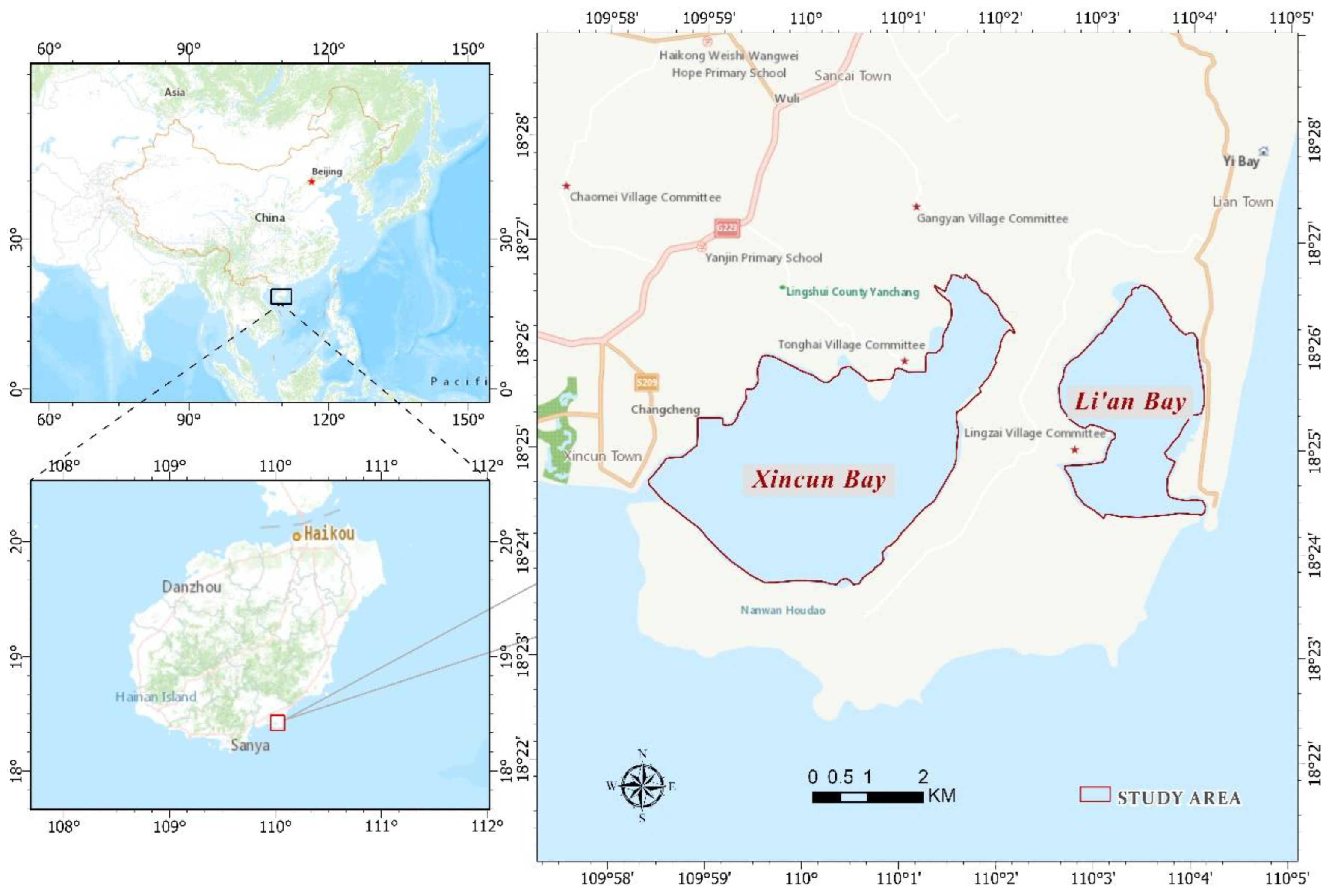
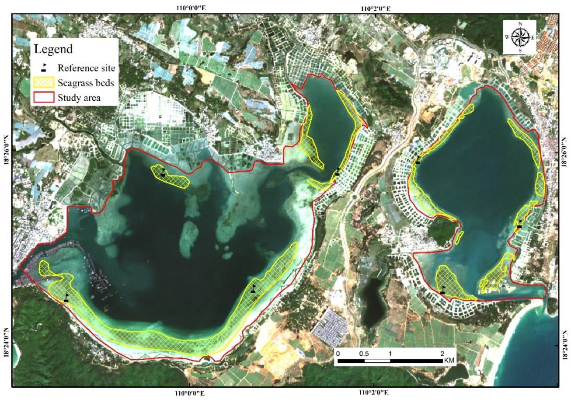
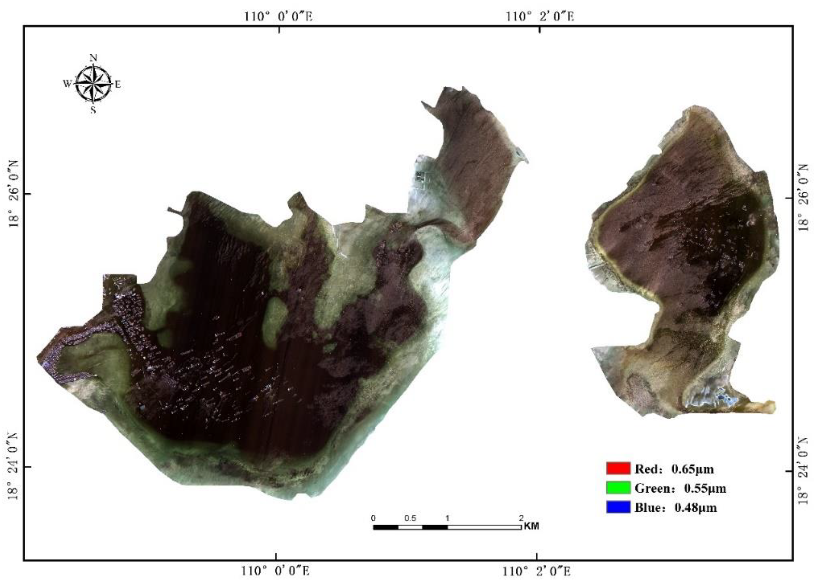
2.1. Location of the Study Area

The study area is located in Xincun Bay, Lingshui County, Hainan Province (109°58′3″E, 18°23′22″N–110°3′52″E, 18°26′57″N) (Figure 1), and was composed of two shallow lagoon basins, namely Xincun Harbor and Li’an Harbor. The water area of Xincun Harbor is about 1731.966 hectares with an average depth of 2.37 m, while the water area of Li’an Harbor is about 714.841 hectares with an average depth of 5.12 m. The seagrasses in this area are widely distributed (Figure 2), with good growth, and with the main species being Enhalus acoroides, Thalassia hemprichii, Cymodocea rotundata, Halodule uninervis, Halophila ovalis, and Halophila minor (Figure 3), among which Enhalus acoroides is the dominant species.

2.2. Image Preprocessing

In this study, a seagrass map for 2020 was created using Chinese Gaofen-2 (GF2) satellite imagery (Table 1), and multi-year change analysis of seagrass spatial distribution was carried out using ESA Sentinel-2 satellite data (Table 2).
The GF2 satellite was successfully launched into its intended orbit on 19 August 2014, and was officially put into service on 6 March 2015. The preprocessing operations performed for GF2 image data include: (1) radiometric calibration and atmospheric correction; (2) water column correction using the bottom reflectance index (BRI) method [42,43]; (3) orthorectification of panchromatic and multispectral bands using the nearest-neighbor sampling method; (4) alignment of the orthorectified multispectral image using the orthorectified panchromatic image as the reference, with the alignment error not exceeding 0.3 pixels; (5) fusion of the aligned 1 m panchromatic image and 4 m multispectral image by the NNDiffuse pan sharpening algorithm to obtain a GF2 image with 1 m spatial resolution; and (6) cropping of the image based on the extent of the study area using the GCS_WGS_1984 coordinate system accompanying the image (Figure 4).
The study area is located in the tropical coastal zone region where the skies in summer and autumn are often covered by tropical cyclone clouds, making it difficult to obtain cloud-free images. However, from November to March each year when the local area enters the dry season, clouds are thin and high-quality images are relatively easy to obtain. Therefore, the Sentinel-2 data in this study were all obtained in the winter of each year (Table 2). Atmospheric correction of the obtained L1-level Sentinel-2 data was performed with a dark spectrum fitting algorithm using ACOLITE software [44,45] (Figure 5 and Figure 6). All bands were resampled to 10 m resolution, and basic preprocessing operations, such as band overlay and image cropping, were performed. It has been demonstrated that Sentinel-2 data can satisfy benthic substrate differentiation by atmospheric correction only [27]; therefore, the Sentinel-2 data in this experiment were not treated with water column correction.

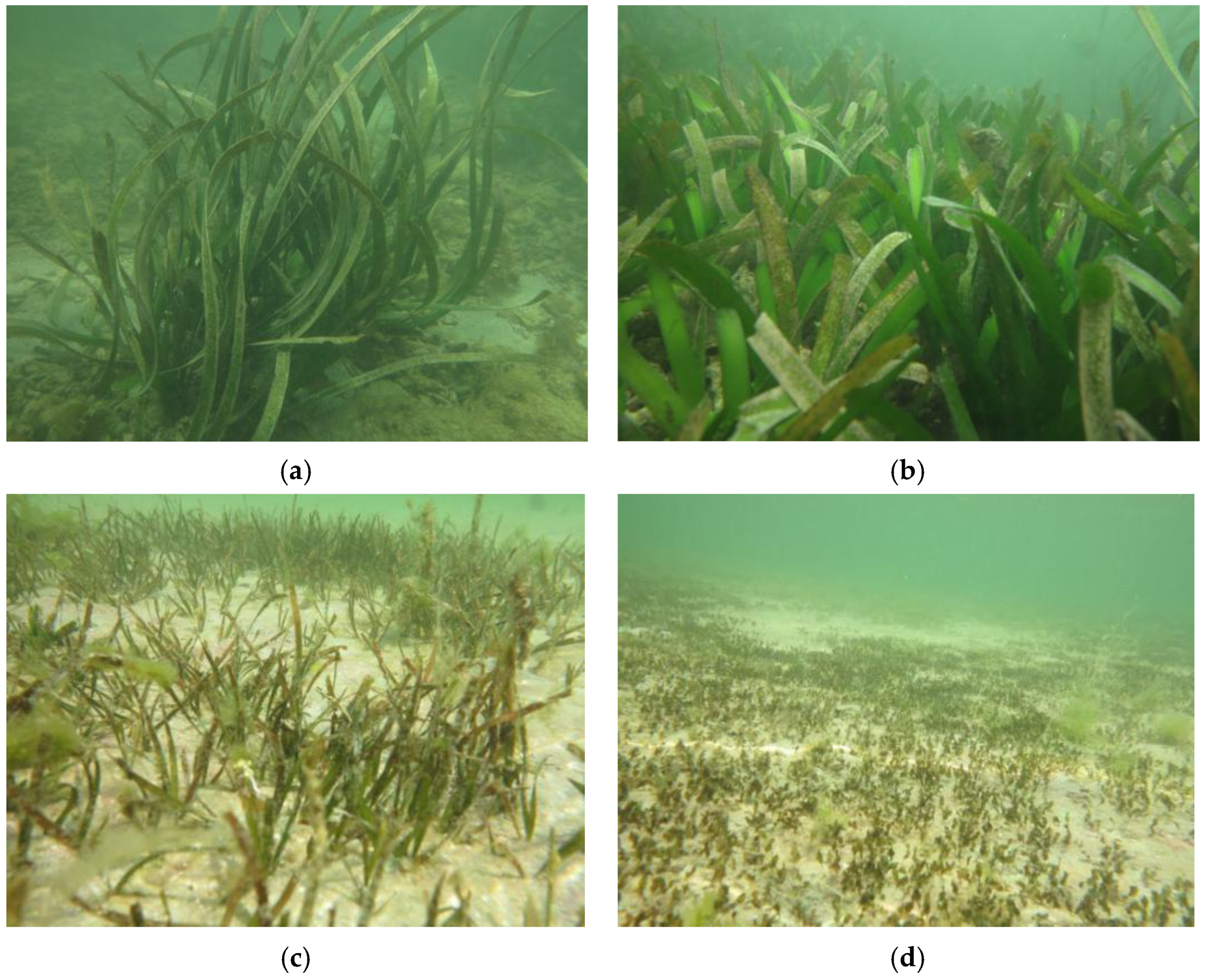
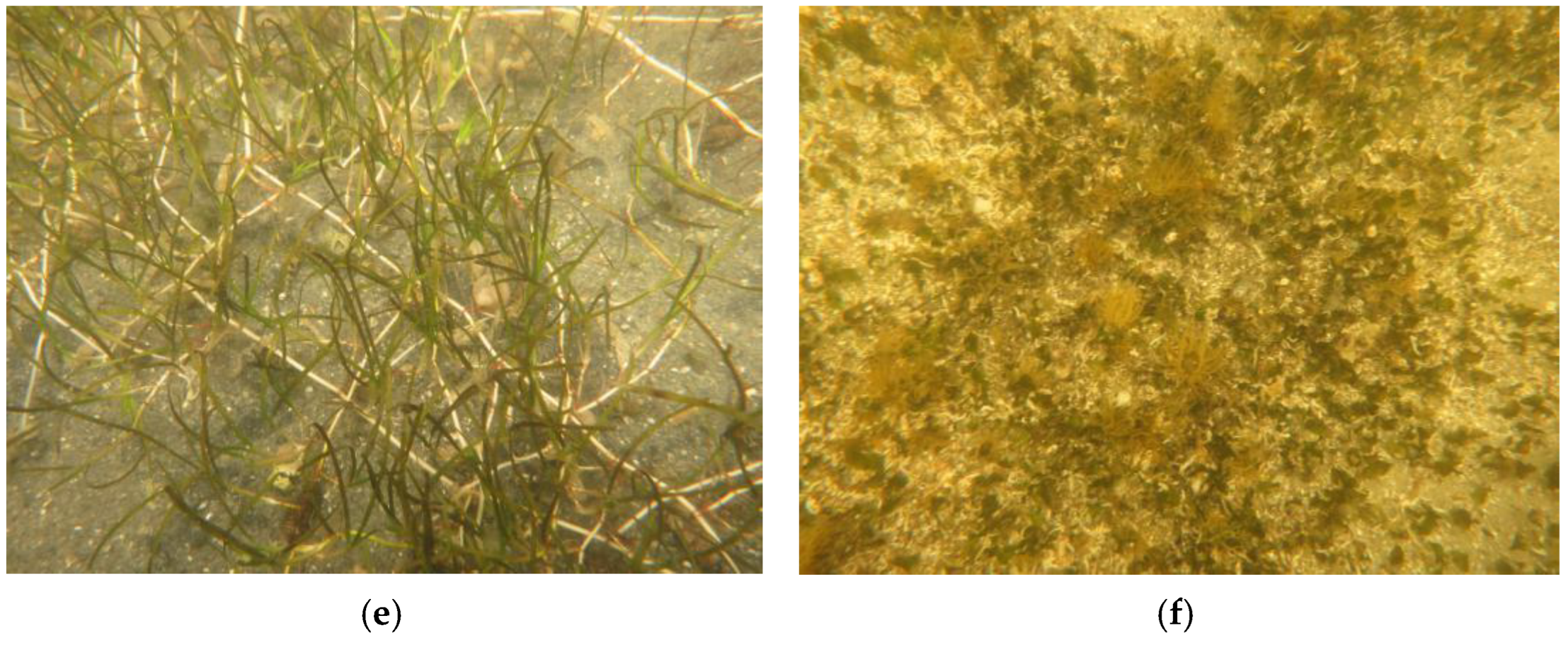
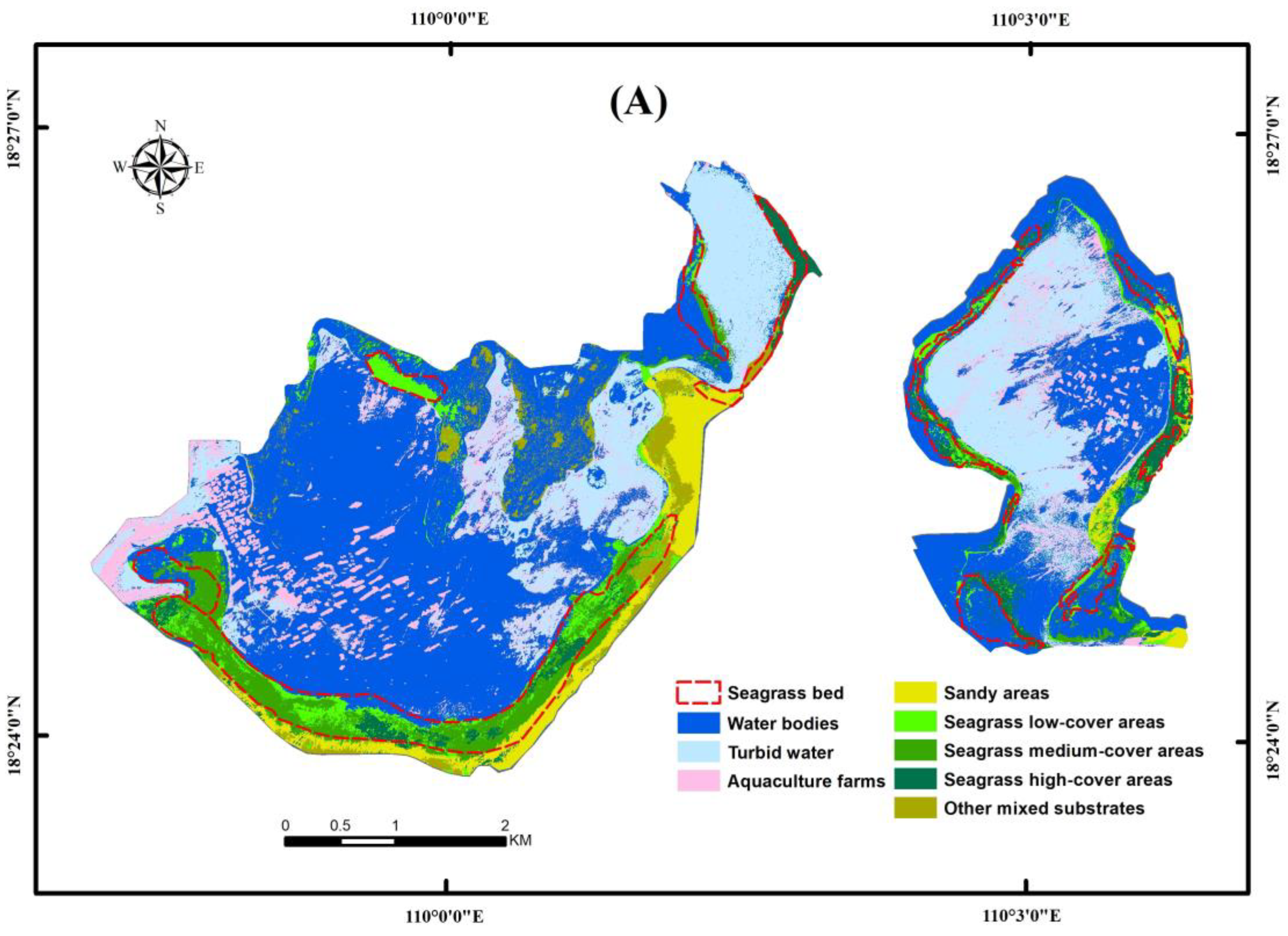
2.3. Classification of Seagrass Distribution Types

The imaging type delineation was based on the results of the 2018 Xincun Seagrass Resource Survey, which was based on the following steps. (1) Lay out the stations, and set up a section at each station. (2) Place a 30.00 × 30.00 cm sample frame, and use an underwater digital camera to photograph the status of seagrass resources in the sample frame. (3) Judge and calculate the seagrass species, density, and cover in the sample frame based on the field survey and filming images.
Based on empirical knowledge of ground truth data and manual interpretation of imagery, the entire study area could be divided in detail into eight types: seagrass high-cover areas, seagrass medium-cover areas, seagrass low-cover areas, sandy areas, other mixed substrates, water bodies, turbid water bodies and polluted waters, and aquaculture farms (Table 3). A 20% seagrass cover was the criterion for distinguishing other substrates from seagrass substrates [46,47], 50% seagrass cover was the criterion for distinguishing low-cover seagrass from medium-cover seagrass, and 80% or more seagrass cover was classified as high-cover seagrass [12,48].
Drawing on the images, the classification of seagrasses into low-, medium-, and high-cover classes was based on the actual size of the three index values of seagrass species, density, and cover at the survey sites, and was combined with the results of image interpretation by seagrass experts to make a comprehensive determination. The steps for selecting samples of seagrass classification pixels are as follows: (1) The location coordinates P(x,y) of the field survey sites were superimposed on the images. (2) Seagrass experts were invited to view the images, to visually estimate the seagrass cover (%) based on the ground truth data and image features at Pi(xi,yi) (Table 4), and to determine the corresponding levels of low-, medium-, and high-seagrass-cover integrated classes. (3) Pixels with the same features near Pi(xi,yi) were selected as part of the classification samples. (4) The levels of seagrass cover (%) near all survey sites were interpreted in turn, and a number of pixels were selected for each of the three integrated classes of low, medium, and high seagrass cover to construct classification samples of seagrass cover. Other types of classification samples were selected directly based on survey visual impressions and visual interpretation of images.

2.4. Image Classification Methods

In this paper, two methods–maximum likelihood and object-oriented image analysis–were used to classify the GF2 images.
Maximum likelihood classification (MLC) is a more mature method for extracting seagrass cover information using remotely sensed imagery and has yielded desirable practical results in many study areas [17,26,29,30]. In this experiment, the preprocessed GF2 data were first subjected to principal component analysis (PCA), and the maximum likelihood method was then executed to classify the data according to the classified samples.
Object-based image analysis (OBIA) is an effective method for monitoring seagrass cover and has been used in recent years for high-resolution remote sensing images [16,19,21,22,31]. One of its important steps is image segmentation, which directly affects the accuracy of classification. In this experiment, the multi-scale segmentation method was chosen to implement segmentation, in order to better avoid the influence of image details and noise compared with other image segmentation methods (Figure 7).

2.5. Error and Accuracy Evaluation

A sample pool was constructed for image classification and to effect the separation of all samples at 1.8 or higher. Pixel sample points were selected based on the location coordinates of the survey sites and on expert empirical knowledge. Based on the pixel sample point locations, the homogeneous spots after image segmentation were selected as the spot samples for the operation of the object-oriented classification method. The selected samples were randomly grouped in a 7:3 ratio for each category, of which 70% were used as training samples for performing classification, and the other 30% were used as validation samples for evaluating the classification accuracy. The accuracy of the classification results was evaluated using the validation samples, and an error matrix and summary table were generated to measure the final classification accuracy using four metrics: overall accuracy, kappa coefficient, mapping accuracy, and user accuracy.

2.6. Spatial and Temporal Variation in Seagrass Distribution

Sentinel-2 image data from the study area for 2016, 2017, 2018, 2019, and 2020 were classified to obtain annual seagrass-cover distribution information. The distribution of seagrasses in each year was compared, and the specific spatial locations where changes occurred were identified. The change area A c h a n g e and the change ratio R a . were calculated to analyze the change status and trends of seagrasses in the study area.
A c h a n g e = A t 1 A t 0
R a = A t 1 A t 0 A t 0 × 100 %

3. Results

3.1. Evaluation of the Accuracy of Seagrass Information Extraction Based on Satellite Images

The classification results based on GF2 image data were evaluated using four indicators: overall accuracy, Kappa coefficient, mapping accuracy, and user accuracy (Table 5 and Table 6). Additionally, the accuracy of seagrass information extraction results based on Sentinel-2 images for the past five years was quantitatively evaluated. It can be seen that in the seagrass-distribution results obtained using GF2 image data, both the MLC and OBIA methods had better accuracy; the OBIA method was especially ideal, able to effectively portray the overall condition of seagrass patches (Figure 8). Better results were also obtained for the seagrass distribution monitoring based on Sentinel-2 imagery for the five years from 2016 to 2020, with overall accuracies of 80.295%, 82.421%, 86.963%, 83.523%, and 84.999%, respectively.

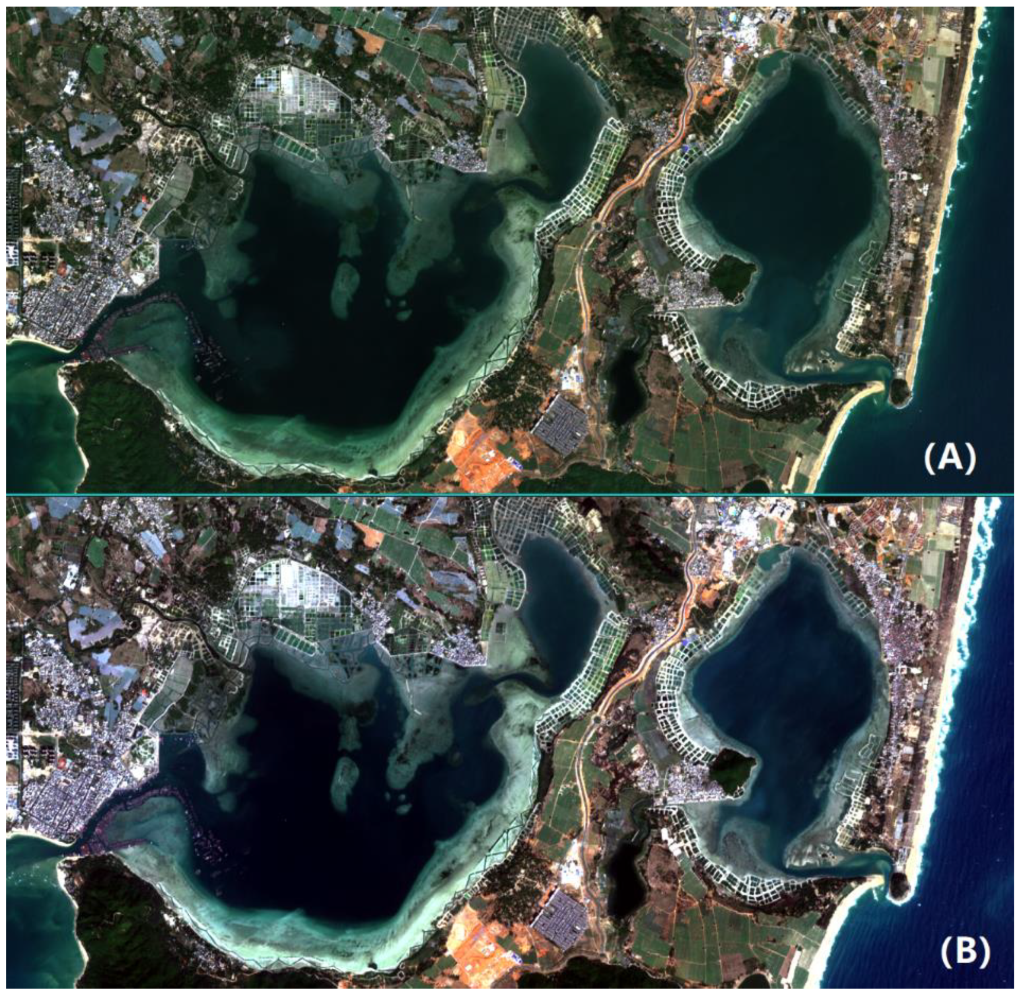
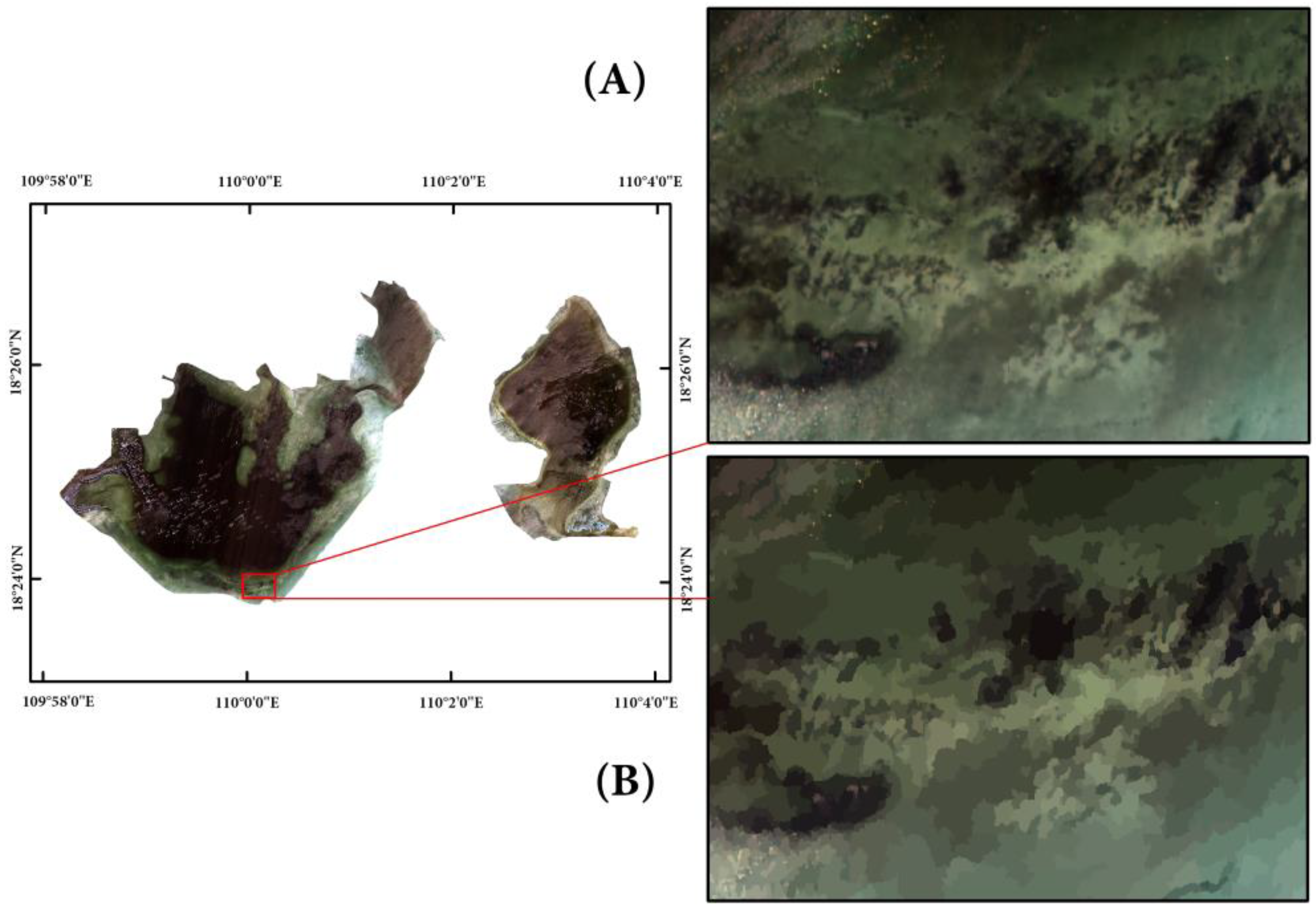
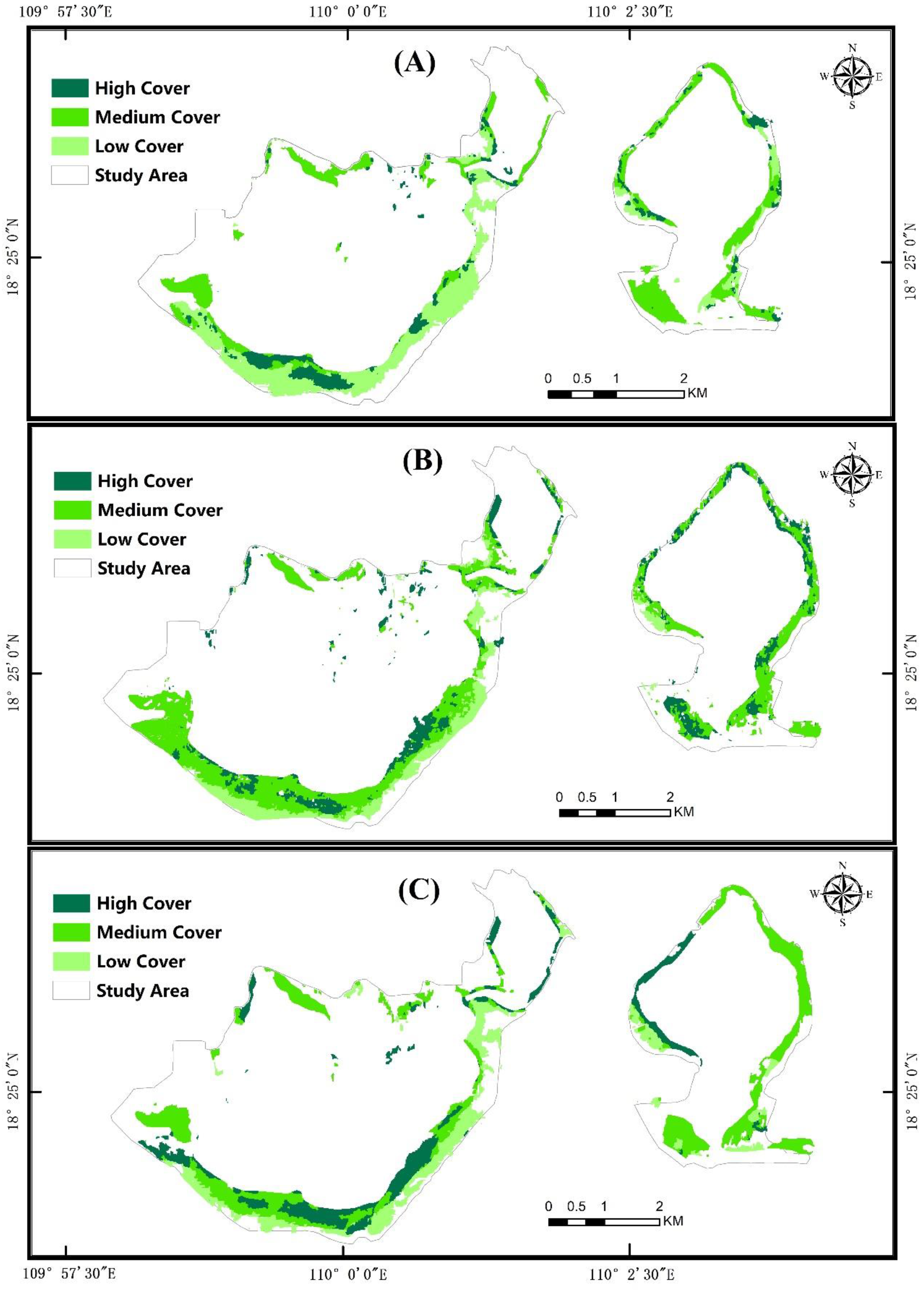
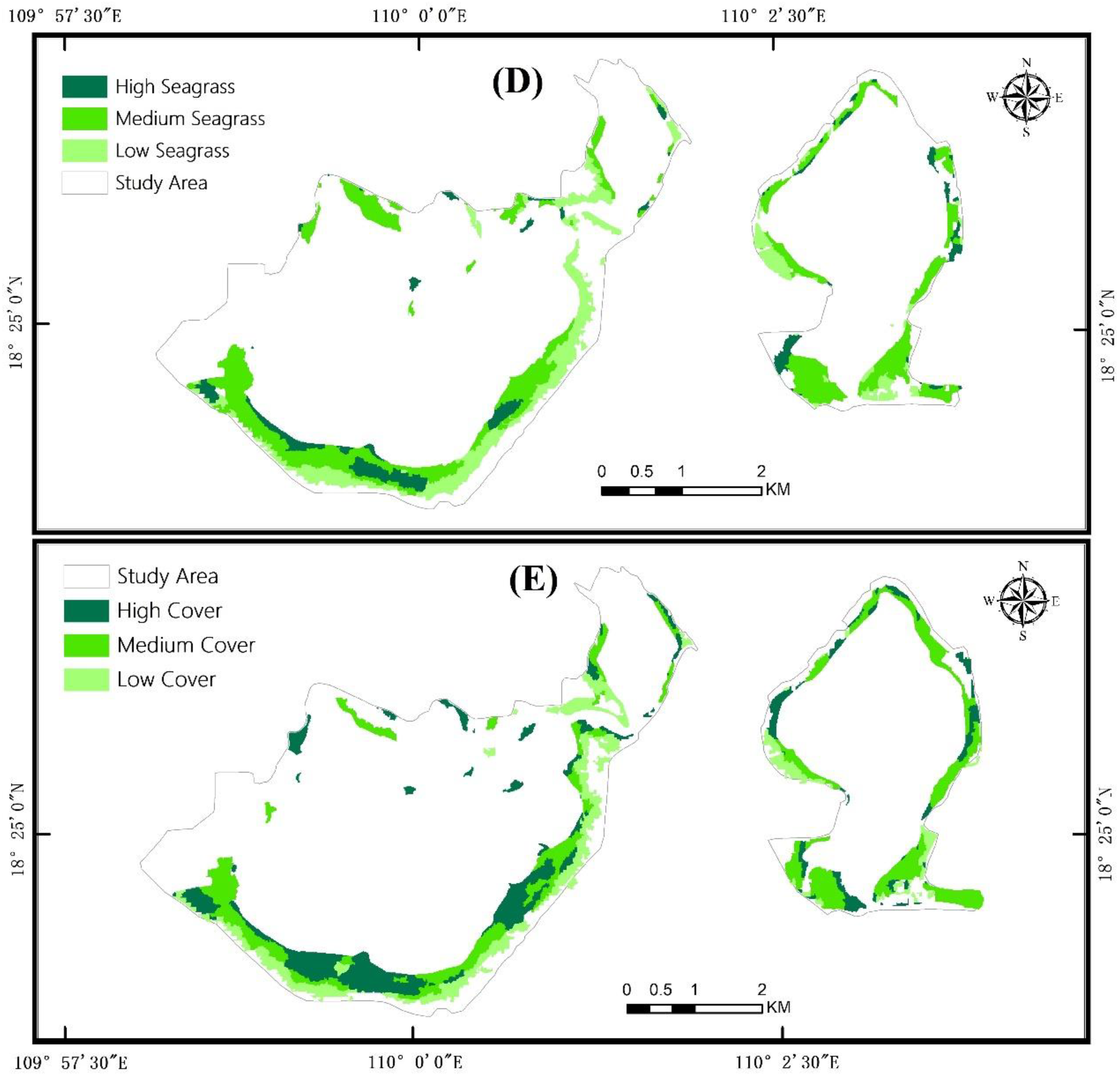
3.2. Mapping of Seagrass Distribution in the Study Area in 2020 Based on GF2 Images

The GF2 image data were analyzed using both the MLC and OBIA methods, and one seagrass distribution map of the study area was obtained for each method (Figure 9). As can be seen from the figure, the main distribution areas of seagrasses obtained by each method were close to the currently known distribution ranges of seagrasses. In addition, both methods revealed many small seagrass patches that had not yet been detected by field surveys. The area status of seagrass distribution in the study area in 2020 was calculated based on the information in the seagrass distribution maps obtained by the OBIA method (Figure 10).

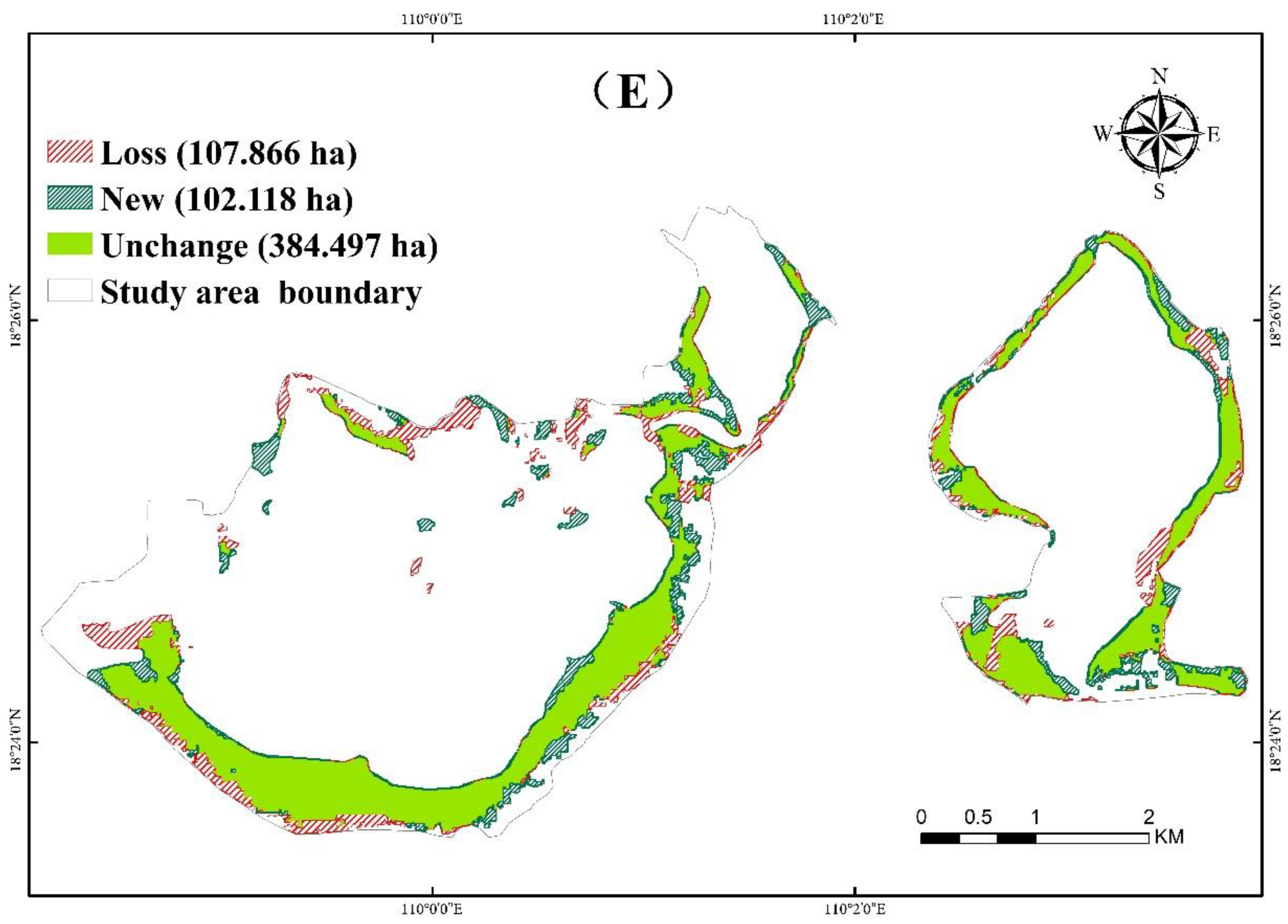
3.3. Mapping of Seagrass Distribution and Changes in the Study Area from 2016 to 2020 Based on Sentinel-2 Imagery

Based on Sentinel-2 data in the study area from 2016 to 2020, seagrass distribution information was extracted for each year (Figure 11). The spatial variation of seagrass distribution during the five years was plotted by comparing the seagrass distribution information from two adjacent years (Figure 12). Based on the mapping results, information related to the distribution of and changes in seagrass areas in the study area from 2016 to 2020 can be statistically obtained (Figure 13, Figure 14, Figure 15 and Figure 16).

4. Discussion

4.1. The Effect of Seagrass Mapping Based on GF2 Images

Spatial resolution is an important factor affecting the accuracy of multispectral satellite remote sensing seagrass monitoring. The higher the spatial resolution of the image, the richer the spatial detail information that can be provided [13,14]. GF2 data can obtain a spatial resolution higher than 1 m through fusion processing, which significantly increases the identifiability of surface objects. GF2 images also have better spectral information characteristics, including the four bands of blue, green, red, and near infrared, in addition to panchromatic bands (Table 1), which are the common ranges for seagrass remote sensing detection [9,49,50,51]. According to the accuracy evaluation, seagrass mapping based on GF2 images can achieve better results.

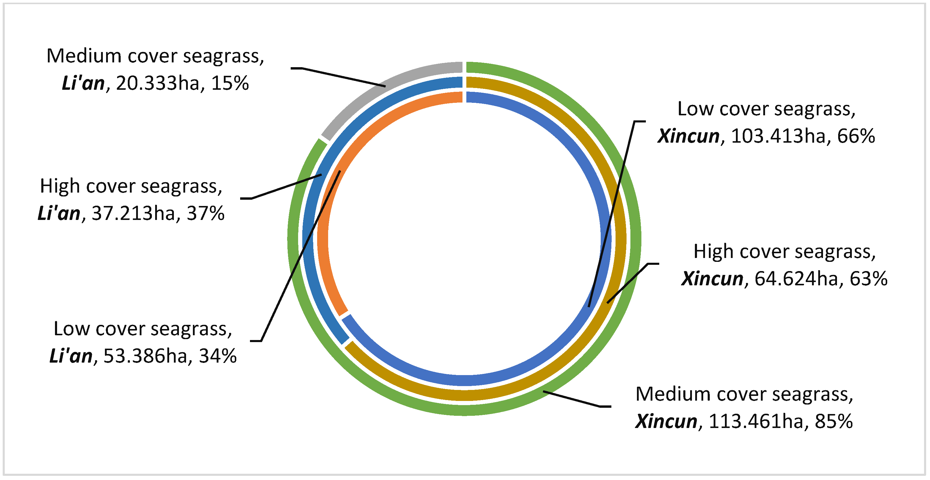
4.2. Status of Seagrass Distribution in the Study Area in 2020

In the statistical image classification results (Figure 9), it can be seen that the total area of seagrass in the study area in 2020 was 392.430 ha. Seagrass in Xincun Harbor was more widely distributed, with 281.498 ha of seagrass area, accounting for about 71.732% of the total seagrass area in the entire study area, while seagrass in Li’an Harbor was distributed across 110.932 ha, accounting for about 28.268% of the total seagrass area in the study area. In terms of spatial distribution, the southern coast of Xincun Harbor is an important area, with seagrasses concentrated and distributed in a strip along the coast. The area of seagrass on this coast was about 228.096 ha, accounting for 79.785% of the seagrass area in Xincun Harbor and 58.124% of the seagrass area in the entire study area. The seagrasses in Li’an Harbor were generally distributed in a narrow strip around the harbor as a whole, sparsely distributed to the north of the harbor, and relatively abundantly distributed in the south, east, and west sides of the harbor, but the overall concentration and contiguity were not as high as those in Xincun Harbor.
The seagrass areas with different coverage levels also differed in the Xincun and Li’an Harbors (Figure 10). Seagrasses with high cover were mainly distributed along the southern coast of Xincun Harbor, forming a concentrated and continuous distribution pattern, while seagrasses with medium cover were distributed continuously along the southern coast of Xincun Harbor and in a large number of continuous areas along the coast of Li’an Harbor, especially in the southern part near the port. The other areas were mainly low-coverage seagrass growing zones but were also interspersed with some small, non-contiguous high-coverage and medium-coverage seagrass areas.

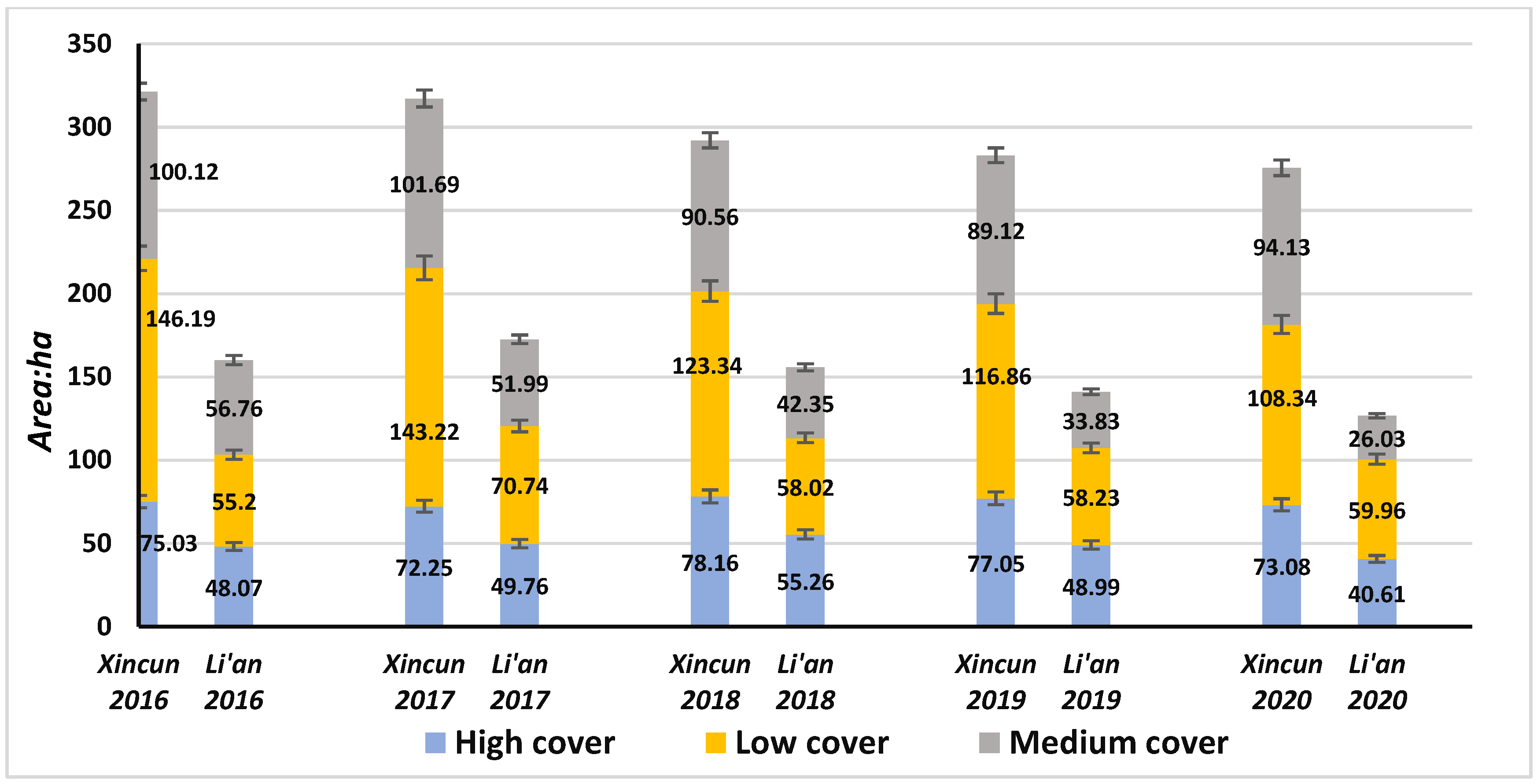
4.3. Spatial and Temporal Variation of Seagrasses in the Study Area from 2016 to 2020

In the images of the statistical seagrass distribution area (Figure 11) and change area (Figure 12) for the five years from 2016 to 2020, it can be seen that the total annual areas of seagrass in the study area were 481.377 ha, 489.652 ha, 447.691 ha, 424.073 ha, and 402.153 ha, respectively. The total area of seagrass decreased by 79.224 ha in five years, with an average annual decrease of 15.844 ha, with the five year decay rate reaching 16.458% with an average decay rate of 3.292% per year. The amount and the rate of change in each specific stage are shown in Figure 13. Among these statistics, the seagrass areas of both the Xincun and Li’an Harbors showed decreasing trends, with reductions of −45.790 ha and −33.430 ha, respectively; the specific change rates of seagrass area of the two harbors in each time period are shown in Figure 14.
During 2016–2017, there were some differences in the changes in seagrass area in the study zone for the three classes of seagrass cover. The seagrass areas with high and medium coverages decreased by 1.093 and 3.200 ha, respectively, while the seagrass area with low coverage increased by 12.571 ha. The area of seagrass distribution for all three levels of cover density showed a decreasing trend from 2018. In particular, the total seagrass area decreased by 41.961 ha during 2017–2018, with the distributed areas of medium- and low-cover seagrass decreasing by 32.664 ha and 20.770 ha, respectively, while the area of high-cover seagrass increased by 11.411 ha. The rate of change in the distribution area of seagrasses with different cover-levels fluctuated between −3.874% and −9.798% during the period 2018–2020 (Figure 15). In general, the area of high-coverage seagrass in the two lagoon harbors in the study area decreased by a total of 9.41 ha during the 5-year period, with a decay rate of 7.644%; the area of medium-coverage seagrass decreased by a total of 36.720 ha during the 5-year period, with a decrease rate of 23.406%; and the area of low-coverage seagrass decreased by a total of 33.091 ha during the 5 year period, with a decrease rate of 16.431%. The changes in seagrass areas with different coverages in the Xincun and Li’an Harbors also had some differences, as shown in Figure 16.

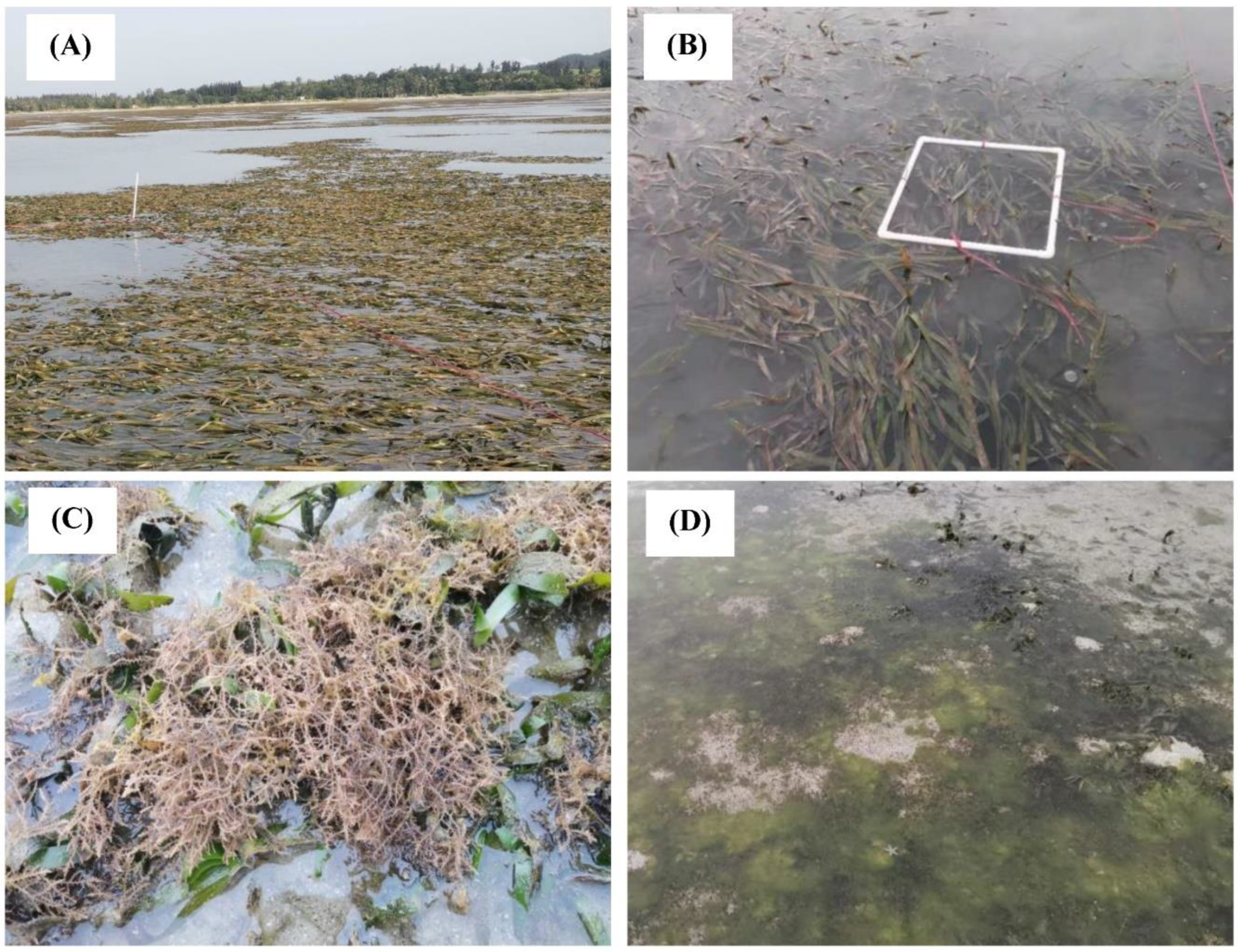
4.4. Main Causes Affecting Seagrass Attenuation in the Study Area

Xincun Bay is the first seagrass nature reserve in China. In the early years, seagrass resources in the two lagoons were abundant and provided important habitats and food resources for commercial and traditional fishery species. In recent years, natural disasters, such as typhoons [52], have had an impact on local seagrass resources, but the significant increase in human activities in the vicinity has been the main cause of the degradation of local seagrass habitats and the decline in seagrass populations [38]. Long-term illegal fishing and extensive aquaculture by nearby fishers have caused serious eutrophication of water bodies in the lagoon, resulting in rapid growth of algae, which severely inhibits the growth and survival of seagrasses [53] (Figure 17) and further affects the function and structure of seagrass communities [54,55]. In addition, coastal discharges and in-lagoon aquaculture have led to increasing levels of heavy metals in the water environment, resulting in a significant increase in the phytotoxic effects of heavy metals on seagrasses [56], thus causing a decline in the number of seagrass plants. These effects have not only reduced the fixation capacity of organic carbon in the seagrass beds of Xincun but also caused the dwindling and degradation of local seagrass habitats [39,40,41].

5. Conclusions

Xincun seagrass is typically representative in terms of seagrass resources and seagrass ecosystems in the South China Sea. It is currently monitored by traditional field research methods, which are time-consuming and inefficient. In this paper, the first monitoring method based on optical satellite remote sensing images was used to comprehensively and rapidly map the distribution of seagrasses in Xincun. Historical changes were projected and analyzed, and three conclusions were obtained. (1) Domestic GF2 images can be applied to seagrass distribution mapping and have good accuracy. (2) Sea grasses in the study area are mostly distributed in Xincun Harbor, with the southern coast of Xincun Harbor being an important area where seagrasses are concentrated and distributed in strips along the coast as a whole. (3) The seagrass area in the study area showed a gradually decreasing trend from 2016 to 2020, and seagrass coverage levels also decreased slowly. Therefore, the development and implementation of specific measures concerning the conservation of seagrass resources should be strengthened. This study was the first comprehensive monitoring of seagrass in Xincun using satellite remote sensing images and comprised the first use of GF2 data in seagrass research, aiming to provide a reference for remote sensing monitoring of seagrass in the South China Sea area and hoping to promote the application of domestic GF2 satellite images for this purpose.

Author Contributions

Conceptualization, Y.L.; Data curation, J.B.; Formal analysis, Y.L. and J.B.; Investigation, Y.L. and J.B.; Project administration, L.Z.; Resources, Z.Y.; Supervision, L.Z. All authors have read and agreed to the published version of the manuscript.

Funding

This research received funding from the Suzhou University of Science and Technology research fund project (XKZ2019009) and Survey of Wetland Resources of International Importance in South China (DDZD20220132).

Acknowledgments

The field survey data used in this research were provided by Bo Huang of Hainan University and Shiquan Chen of the Hainan Academy of Marine and Fishery Sciences. We express our sincere thanks to them. We would also like to thank Xiaohai Zhang and Weipin Ding for providing field photos.

Conflicts of Interest

The authors declare no conflict of interest.

References

  1. Unsworth, R.K.F.; McKenzie, L.J.; Collier, C.J.; Cullen-Unsworth, L.C.; Duarte, C.M.; Eklöf, J.S.; Jarvis, J.C.; Jones, B.L.; Nordlund, L.M. Global challenges for seagrass conservation. Ambio 2019, 48, 801–815. [Google Scholar] [CrossRef] [PubMed] [Green Version]
  2. McKenzie, L.J.; Nordlund, L.M.; Jones, B.L.; Cullen-Unsworth, L.C.; Roelfsema, C.; Unsworth, R.K.F. The global distribution of seagrass meadows. Environ. Res. Lett. 2020, 15, 74041. [Google Scholar] [CrossRef]
  3. Potouroglou, M.; Bull, J.C.; Krauss, K.W.; Kennedy, H.A.; Fusi, M.; Daffonchio, D.; Mangora, M.M.; Githaiga, M.N.; Diele, K.; Huxham, M. Measuring the role of seagrasses in regulating sediment surface elevation. Sci. Rep. 2017, 7, 11917. [Google Scholar] [CrossRef] [Green Version]
  4. Fourqurean, J.W.; Duarte, C.M.; Kennedy, H.; Marbà, N.; Holmer, M.; Mateo, M.A.; Apostolaki, E.T.; Kendrick, G.A.; Krause-Jensen, D.; McGlathery, K.J.; et al. Seagrass ecosystems as a globally significant carbon stock. Nat. Geosci. 2012, 5, 505–509. [Google Scholar] [CrossRef]
  5. Green, A.E.; Unsworth, R.K.F.; Chadwick, M.A.; Jones, P.J.S. Historical Analysis Exposes Catastrophic Seagrass Loss for the United Kingdom. Front. Plant Sci. 2021, 12, 261. [Google Scholar] [CrossRef]
  6. Short, F.T.; Polidoro, B.; Livingstone, S.R.; Carpenter, K.E.; Bandeira, S.; Bujang, J.S.; Calumpong, H.P.; Carruthers, T.J.B.; Coles, R.G.; Dennison, W.C.; et al. Extinction risk assessment of the world’s seagrass species. Biol. Conserv. 2011, 144, 1961–1971. [Google Scholar] [CrossRef]
  7. De la Torre-Castro, M.; Di Carlo, G.; Jiddawi, N.S. Seagrass importance for a small-scale fishery in the tropics: The need for seascape management. Mar. Pollut. Bull. 2014, 83, 398–407. [Google Scholar] [CrossRef]
  8. Nordlund, L.M.; Unsworth, R.K.F.; Gullström, M.; Cullen-Unsworth, L.C. Global significance of seagrass fishery activity. Fish Fish. 2018, 19, 399–412. [Google Scholar] [CrossRef]
  9. Hossain, M.S.; Bujang, J.S.; Zakaria, M.H.; Hashim, M. The application of remote sensing to seagrass ecosystems: An overview and future research prospects. Int. J. Remote Sens. 2015, 36, 61–114. [Google Scholar] [CrossRef]
  10. Veettil, B.K.; Ward, R.D.; Lima, M.D.A.C.; Stankovic, M.; Hoai, P.N.; Quang, N.X. Opportunities for seagrass research derived from remote sensing: A review of current methods. Ecol. Indic. 2020, 117, 106560. [Google Scholar] [CrossRef]
  11. Murray, N.J.; Keith, D.A.; Bland, L.M.; Ferrari, R.; Lyons, M.B.; Lucas, R.; Pettorelli, N.; Nicholson, E. The role of satellite remote sensing in structured ecosystem risk assessments. Sci. Total Environ. 2018, 619–620, 249–257. [Google Scholar] [CrossRef] [PubMed] [Green Version]
  12. Zoffoli, M.L.; Gernez, P.; Godet, L.; Peters, S.; Oiry, S.; Barillé, L. Decadal increase in the ecological status of a North-Atlantic intertidal seagrass meadow observed with multi-mission satellite time-series. Ecol. Indic. 2021, 130, 108033. [Google Scholar] [CrossRef]
  13. Wicaksono, P.; Salivian Wisnu Kumara, I.; Kamal, M.; Afif Fauzan, M.; Zhafarina, Z.; Agus Nurswantoro, D.; Noviaris Yogyantoro, R. Multispectral Resampling of Seagrass Species Spectra: WorldView-2, Quickbird, Sentinel-2A, ASTER VNIR, and Landsat 8 OLI. IOP conference series. Earth Environ. Sci. 2017, 98, 12039. [Google Scholar] [CrossRef]
  14. Kovacs, E.; Roelfsema, C.; Lyons, M.; Zhao, S.; Phinn, S. Seagrass habitat mapping: How do Landsat 8 OLI, Sentinel-2, ZY-3A, and Worldview-3 perform? Remote Sens. Lett. 2018, 9, 686–695. [Google Scholar] [CrossRef]
  15. Garcia, R.; Hedley, J.; Tin, H.; Fearns, P. A Method to Analyze the Potential of Optical Remote Sensing for Benthic Habitat Mapping. Remote Sens. 2015, 7, 13157–13189. [Google Scholar] [CrossRef] [Green Version]
  16. Baumstark, R.; Duffey, R.; Pu, R. Mapping seagrass and colonized hard bottom in Springs Coast, Florida using WorldView-2 satellite imagery. Estuar. Coast. Shelf Sci. 2016, 181, 83–92. [Google Scholar] [CrossRef]
  17. Pu, R.; Bell, S. Mapping seagrass coverage and spatial patterns with high spatial resolution IKONOS imagery. Int. J. Appl. Earth Obs. Geoinf. 2017, 54, 145–158. [Google Scholar] [CrossRef]
  18. Poursanidis, D.; Topouzelis, K.; Chrysoulakis, N. Mapping coastal marine habitats and delineating the deep limits of the Neptune’s seagrass meadows using very high resolution Earth observation data. Int. J. Remote Sens. 2018, 39, 8670–8687. [Google Scholar] [CrossRef]
  19. Siregar, V.P.; Agus, S.B.; Subarno, T.; Prabowo, N.W. Mapping shallow waters habitats using OBIA by applying several approaches of depth invariant index in North Kepulauan Seribu. IOP conference series. Earth Environ. Sci. 2018, 149, 12052. [Google Scholar]
  20. Wicaksono, P.; Lazuardi, W. Assessment of PlanetScope images for benthic habitat and seagrass species mapping in a complex optically shallow water environment. Int. J. Remote Sens. 2018, 39, 5739–5765. [Google Scholar] [CrossRef]
  21. Papakonstantinou, A.; Stamati, C.; Topouzelis, K. Comparison of True-Color and Multispectral Unmanned Aerial Systems Imagery for Marine Habitat Mapping Using Object-Based Image Analysis. Remote Sens. 2020, 12, 554. [Google Scholar] [CrossRef] [Green Version]
  22. Rende, S.F.; Bosman, A.; Di Mento, R.; Bruno, F.; Lagudi, A.; Irving, A.D.; Dattola, L.; Giambattista, L.D.; Lanera, P.; Proietti, R.; et al. Ultra-High-Resolution Mapping of Posidonia oceanica (L.) Delile Meadows through Acoustic, Optical Data and Object-based Image Classification. J. Mar. Sci. Eng. 2020, 8, 647. [Google Scholar] [CrossRef]
  23. Traganos, D.; Reinartz, P. Mapping Mediterranean seagrasses with Sentinel-2 imagery. Mar. Pollut. Bull. 2018, 134, 197–209. [Google Scholar] [CrossRef] [PubMed] [Green Version]
  24. Traganos, D.; Reinartz, P. Machine learning-based retrieval of benthic reflectance and Posidonia oceanica seagrass extent using a semi-analytical inversion of Sentinel-2 satellite data. Int. J. Remote Sens. 2018, 39, 9428–9452. [Google Scholar] [CrossRef]
  25. Immordino, F.; Barsanti, M.; Candigliota, E.; Cocito, S.; Delbono, I.; Peirano, A. Application of Sentinel-2 Multispectral Data for Habitat Mapping of Pacific Islands: Palau Republic (Micronesia, Pacific Ocean). J. Mar. Sci. Eng. 2019, 7, 316. [Google Scholar] [CrossRef] [Green Version]
  26. Ha, N.T.; Manley-Harris, M.; Pham, T.D.; Hawes, I. A Comparative Assessment of Ensemble-Based Machine Learning and Maximum Likelihood Methods for Mapping Seagrass Using Sentinel-2 Imagery in Tauranga Harbor, New Zealand. Remote Sens. 2020, 12, 355. [Google Scholar] [CrossRef] [Green Version]
  27. Kuhwald, K.; Schneider Von Deimling, J.; Schubert, P.; Oppelt, N. How can Sentinel-2 contribute to seagrass mapping in shallow, turbid Baltic Sea waters? Remote Sens. Ecol. Conserv. 2021. [Google Scholar] [CrossRef]
  28. Zoffoli, M.L.; Gernez, P.; Rosa, P.; Le Bris, A.; Brando, V.E.; Barillé, A.; Harin, N.; Peters, S.; Poser, K.; Spaias, L.; et al. Sentinel-2 remote sensing of Zostera noltei-dominated intertidal seagrass meadows. Remote Sens. Environ. 2020, 251, 112020. [Google Scholar] [CrossRef]
  29. Meyer, C.A.; Pu, R. Seagrass resource assessment using remote sensing methods in St. Joseph Sound and Clearwater Harbor, Florida, USA. Environ. Monit. Assess. 2012, 184, 1131–1143. [Google Scholar] [CrossRef]
  30. Pu, R.; Bell, S.; Meyer, C. Mapping and assessing seagrass bed changes in Central Florida’s west coast using multitemporal Landsat TM imagery. Estuar. Coast. Shelf Sci. 2014, 149, 68–79. [Google Scholar] [CrossRef]
  31. Ventura, D.; Bonifazi, A.; Gravina, M.F.; Belluscio, A.; Ardizzone, G. Mapping and Classification of Ecologically Sensitive Marine Habitats Using Unmanned Aerial Vehicle (UAV) Imagery and Object-Based Image Analysis (OBIA). Remote Sens. 2018, 10, 1331. [Google Scholar] [CrossRef] [Green Version]
  32. Fengying, Z.; Guanglong, Q.; Hangqing, F.; Wei, Z. Diversity, distribution and conservation of Chinese seagrass species:Diversity, distribution and conservation of Chinese seagrass species. Biodivers. Sci. 2013, 21, 571. [Google Scholar]
  33. Huang, X.; Huang, L.; Li, Y.; Xu, Z.; Fong, C.W.; Huang, D.; Han, Q.; Huang, H.; Tan, Y.; Liu, S. Main seagrass beds and threats to their habitats in the coastal sea of South China. Chin. Sci. Bull. 2006, 51 (Suppl. S2), 136–142. [Google Scholar] [CrossRef]
  34. Xiao, X.; Huang, Y.; Holmer, M. Current trends in seagrass research in China (2010–2019). Aquat. Bot. 2020, 166, 103266. [Google Scholar] [CrossRef]
  35. Sudo, K.; Quiros, T.E.A.L.; Prathep, A.; Luong, C.V.; Lin, H.; Bujang, J.S.; Ooi, J.L.S.; Fortes, M.D.; Zakaria, M.H.; Yaakub, S.M.; et al. Distribution, Temporal Change, and Conservation Status of Tropical Seagrass Beds in Southeast Asia: 2000–2020. Front. Mar. Sci. 2021, 8, 779. [Google Scholar] [CrossRef]
  36. Yang, D.; Yang, C. Detection of Seagrass Distribution Changes from 1991 to 2006 in Xincun Bay, Hainan, with Satellite Remote Sensing. Sensors 2009, 9, 830–844. [Google Scholar] [CrossRef]
  37. Xu, S.; Xu, S.; Zhou, Y.; Yue, S.; Zhang, X.; Gu, R.; Zhang, Y.; Qiao, Y.; Liu, M. Long-Term Changes in the Unique and Largest Seagrass Meadows in the Bohai Sea (China) Using Satellite (1974–2019) and Sonar Data: Implication for Conservation and Restoration. Remote Sens. 2021, 13, 856. [Google Scholar] [CrossRef]
  38. Zhang, J.; Huang, X.; Jiang, Z. Physiological responses of the seagrass Thalassia hemprichii (Ehrenb.) Aschers as indicators of nutrient loading. Mar. Pollut. Bull. 2014, 83, 508–515. [Google Scholar] [CrossRef]
  39. Jiang, Z.; Liu, S.; Zhang, J.; Wu, Y.; Zhao, C.; Lian, Z.; Huang, X. Eutrophication indirectly reduced carbon sequestration in a tropical seagrass bed. Plant Soil 2018, 426, 135–152. [Google Scholar] [CrossRef]
  40. Liu, S.; Jiang, Z.; Wu, Y.; Zhang, J.; Arbi, I.; Ye, F.; Huang, X.; Macreadie, P.I. Effects of nutrient load on microbial activities within a seagrass-dominated ecosystem: Implications of changes in seagrass blue carbon. Mar. Pollut. Bull. 2017, 117, 214–221. [Google Scholar] [CrossRef]
  41. Liu, S.; Jiang, Z.; Deng, Y.; Wu, Y.; Zhang, J.; Zhao, C.; Huang, D.; Huang, X.; Trevathan-Tackett, S.M. Effects of nutrient loading on sediment bacterial and pathogen communities within seagrass meadows. MicrobiologyOpen 2018, 7, e00600. [Google Scholar] [CrossRef] [PubMed]
  42. Sagawa, T.; Boisnier, E.; Komatsu, T.; Mustapha, K.B.; Hattour, A.; Kosaka, N.; Miyazaki, S. Using bottom surface reflectance to map coastal marine areas: A new application method for Lyzenga’s model. Int. J. Remote Sens. 2010, 31, 3051–3064. [Google Scholar] [CrossRef]
  43. Chen, C.; Lau, V.; Chang, N.; Son, N.; Tong, P.; Chiang, S. Multi-temporal change detection of seagrass beds using integrated Landsat TM/ETM+/OLI imageries in Cam Ranh Bay, Vietnam. Ecol. Inform. 2016, 35, 43–54. [Google Scholar] [CrossRef]
  44. Vanhellemont, Q. Adaptation of the dark spectrum fitting atmospheric correction for aquatic applications of the Landsat and Sentinel-2 archives. Remote Sens. Environ. 2019, 225, 175–192. [Google Scholar] [CrossRef]
  45. Vanhellemont, Q.; Ruddick, K. Atmospheric correction of metre-scale optical satellite data for inland and coastal water applications. Remote Sens. Environ. 2018, 216, 586–597. [Google Scholar] [CrossRef]
  46. Valle, M.; Palà, V.; Lafon, V.; Dehouck, A.; Garmendia, J.M.; Borja, Á.; Chust, G. Mapping estuarine habitats using airborne hyperspectral imagery, with special focus on seagrass meadows. Estuar. Coast. Shelf Sci. 2015, 164, 433–442. [Google Scholar] [CrossRef]
  47. Barillé, L.; Robin, M.; Harin, N.; Bargain, A.; Launeau, P. Increase in seagrass distribution at Bourgneuf Bay (France) detected by spatial remote sensing. Aquat. Bot. 2010, 92, 185–194. [Google Scholar] [CrossRef]
  48. Calleja, F.; Galván, C.; Silió-Calzada, A.; Juanes, J.A.; Ondiviela, B. Long-term analysis of Zostera noltei: A retrospective approach for understanding seagrasses’ dynamics. Mar. Environ. Res. 2017, 130, 93–105. [Google Scholar] [CrossRef]
  49. Lyzenga, D.R. Passive remote sensing techniques for mapping water depth and bottom features. Appl. Opt. 1978, 17, 379. [Google Scholar] [CrossRef]
  50. Kim, K.; Choi, J.; Ryu, J.; Jeong, H.J.; Lee, K.; Park, M.G.; Kim, K.Y. Observation of typhoon-induced seagrass die-off using remote sensing. Estuar. Coast. Shelf Sci. 2015, 154, 111–121. [Google Scholar] [CrossRef]
  51. Wicaksono, P.; Fauzan, M.A.; Kumara, I.S.W.; Yogyantoro, R.N.; Lazuardi, W.; Zhafarina, Z. Analysis of reflectance spectra of tropical seagrass species and their value for mapping using multispectral satellite images. Int. J. Remote Sens. 2019, 40, 8955–8978. [Google Scholar] [CrossRef]
  52. Yang, D.; Huang, D. Impacts of Typhoons Tianying and Dawei on seagrass distribution in Xincun Bay, Hainan Province, China. Acta Oceanol. Sin. 2011, 30, 32–39. [Google Scholar] [CrossRef]
  53. Hauxwell, J.; Cebrián, J.; Valiela, I. Eelgrass Zostera marina loss in temperate estuaries: Relationship to land-derived nitrogen loads and effect of light limitation imposed by algae. Mar. Ecol. Prog. Ser. 2003, 247, 59–73. [Google Scholar] [CrossRef] [Green Version]
  54. Ruiz, J.M.; Marco-Méndez, C.; Sánchez-Lizaso, J.L. Remote influence of off-shore fish farm waste on Mediterranean seagrass (Posidonia oceanica) meadows. Mar. Environ. Res. 2010, 69, 118–126. [Google Scholar] [CrossRef] [PubMed]
  55. Fertig, B.; Kennish, M.J.; Sakowicz, G.P. Changing eelgrass (Zostera marina L.) characteristics in a highly eutrophic temperate coastal lagoon. Aquat. Bot. 2013, 104, 70–79. [Google Scholar] [CrossRef]
  56. Zheng, J.; Gu, X.; Zhang, T.; Liu, H.; Ou, Q.; Peng, C. Phytotoxic effects of Cu, Cd and Zn on the seagrass Thalassia hemprichii and metal accumulation in plants growing in Xincun Bay, Hainan, China. Ecotoxicology 2018, 27, 517–526. [Google Scholar] [CrossRef]
Figure 1. Location of the study area (working base map from ArcGIS Pro’s colorful English version of the Chinese map. Projection: WGS 1984 Web Mercator).
Remotesensing 14 02373 g001
Figure 2. Distribution of seagrasses in the study area with the surface conditions displayed by the Sentinel-2 images (28 December 2020).
Remotesensing 14 02373 g002
Figure 3. Seagrass species in the study area. (a) E. acoroides (b) T. hemprichii (c) C. rotundata (d) H. ovalis (e) H. uninervis (f) H. minor.
Remotesensing 14 02373 g003aRemotesensing 14 02373 g003b
Figure 4. GF2 image data (10 August 2020) of the study area after preprocessing.
Remotesensing 14 02373 g004
Figure 5. Comparison between the image after atmospheric correction using the ACOLITE method and the original image ((A) is the original image, and (B) is the image after ACOLITE atmospheric correction).
Remotesensing 14 02373 g005
Figure 6. Comparison of the localized image after atmospheric correction using the ACOLITE method with the localized original image ((A) is the localized original image, and (B) is the localized image after ACOLITE atmospheric correction). (Taking the 2020 Sentinel-2 image as an example, the seagrass information on the image is more obvious after the ACOLITE atmospheric correction).
Remotesensing 14 02373 g006
Figure 7. Comparison of original and segmented images of GF2 data in the study area ((A) original image and (B) segmented image).
Remotesensing 14 02373 g007
Figure 8. Comparison of the results of seagrass information extraction by two methods ((A) results of the MLC method and (B) results of the OBIA method).
Remotesensing 14 02373 g008
Figure 9. Seagrass map based on the MLC and OBIA methods ((A) results of the MLC method and (B) results of the OBIA method).
Remotesensing 14 02373 g009aRemotesensing 14 02373 g009b
Figure 10. Area and percentage of seagrass with different cover classes in Xincun Harbor and Li’an Harbor in 2020.
Remotesensing 14 02373 g010
Figure 11. Annual map of seagrass distribution in the study area ((A) 2016, (B) 2017, (C) 2018, (D) 2019, and (E) 2020).
Remotesensing 14 02373 g011aRemotesensing 14 02373 g011b
Figure 12. Annual changes in seagrass distribution in the study area ((A) 2016–2017, (B) 2017–2018, (C) 2018–2019, (D) 2019–2020, and (E) 2016–2020).
Remotesensing 14 02373 g012aRemotesensing 14 02373 g012bRemotesensing 14 02373 g012c
Figure 13. Amount and rate of seagrass area changes in the study area from 2016 to 2020.
Remotesensing 14 02373 g013
Figure 14. Change rate of seagrass area (%) between 2016 and 2020 in the Xincun and Li’an Harbors.
Remotesensing 14 02373 g014
Figure 15. Change rate of the seagrass area in the study area from 2016 to 2020 for three cover levels.
Remotesensing 14 02373 g015
Figure 16. Seagrass area statistics with different cover in the Xincun and Li’an Harbors during 2016–2020.
Remotesensing 14 02373 g016
Figure 17. Healthy growing seagrasses vs. algae-affected seagrass in Xincun Bay ((A) continuous growth of E. acoroides, (B) healthy growth of E. acoroides, (C) T. hemprichii inhibited by algae, and (D) H. ovalis and T. hemprichii in decline due to algal influence).
Remotesensing 14 02373 g017
Table 1. GF2 satellite image data used in the study.
Band No.Spectral BandSpectral Range
(μm)
Spatial Resolution (m)Width (km)Experimental Data Date
PA1Panchromatic0.45–0.9014510 August 2020
MSI2Blue0.45–0.524
3Green0.52–0.59
4Red0.63–0.69
5NIR0.77–0.89
Table 2. Sentinel-2 satellite image data used for the study.
Band No.Spectral BandCentral Wavelength (μm)Spatial Resolution (m)Experimental Data Date
1Coastal aerosol0.443609 December 2016
19 December 2017
30 October 2018
4 December 2019
28 December 2020
2Blue0.49010
3Green0.56010
4Red0.66510
5Vegetation red edge0.70520
6Vegetation red edge0.74020
7Vegetation red edge0.78320
8NIR0.84210
8ANarrow NIR0.86520
9Water vapor0.94560
11SWIR1.61020
12SWIR2.19020
Table 3. Classification of study area types.
Class TypeDescription
Seagrass high-cover areas>80% seagrass coverage in the pixel
Seagrass medium-cover areas>50%, <80% seagrass coverage in the pixel
Seagrass low-cover areas>20%, <50% seagrass coverage in the pixel
Sandy areas<20% seagrass, >80% bare sand coverage in the pixel
Other mixed substratesMixed coverages of very little seagrass, seaweed, sand, and gravel in the pixel
Water bodiesThe water body area
Turbid water bodiesTurbid water body and polluted water area
Aquaculture farmsFishing rafts and nets area used for aquaculture
Table 4. Manual visual estimation of seagrass cover based on image features.
DataImage FeaturesVisual Estimation of Seagrass Coverage (%)Image FeaturesVisual Estimation of Seagrass Coverage (%)Image FeaturesVisual Estimation of Seagrass Coverage (%)
Sentinel-2 Remotesensing 14 02373 i001100% Remotesensing 14 02373 i00276% Remotesensing 14 02373 i00335%
GF2 Remotesensing 14 02373 i00495% Remotesensing 14 02373 i00575% Remotesensing 14 02373 i00640%
Sentinel-2 Remotesensing 14 02373 i00788% Remotesensing 14 02373 i00855% Remotesensing 14 02373 i00920%
GF2 Remotesensing 14 02373 i01086% Remotesensing 14 02373 i01157% Remotesensing 14 02373 i01225%
Table 5. Classification result accuracy of MLC.
ClassProd. Acc. (Percent)User Acc. (Percent)Prod. Acc. (Pixels)User Acc. (Pixels)
Water bodies91.7183.012986/32562986/3597
Turbid Water bodies82.1876.48959/1167959/1254
Aquaculture farms73.6376.51863/1172963/1128
Seagrass high-cover areas77.4886.211338/17271338/1552
Seagrass low-cover areas77.9863.161190/15261190/1884
Seagrass medium-cover areas56.9397.21698/1226698/718
Sandy areas10073.861023/10231023/1385
Other mixed substrates43.7274.09449/1027449/606
Overall Accuracy(9506/12,124) = 78.407%
Kappa Coefficient0.744
Table 6. Classification result accuracy of OBIA.
ClassProd. Acc. (Percent)User Acc. (Percent)Prod. Acc. (Pixels)User Acc. (Pixels)
Water bodies95.1477.23074/32313074/3982
Turbid Water bodies81.2190.38977/1203977/1081
Aquaculture farms79.294.73952/1202952/1005
Seagrass high-cover areas91.292.041503/16481503/1633
Seagrass low-cover areas82.0881.751232/15011232/1507
Seagrass medium-cover areas65.55100805/1228805/805
Sandy areas10064.781008/10081008/1556
Other mixed substrates45.42100456/1004456/456
Overall Accuracy(10,007/12,025) = 83.218%
Kappa Coefficient0.7999
Publisher’s Note: MDPI stays neutral with regard to jurisdictional claims in published maps and institutional affiliations.

