Backtracking Reconstruction Network for Three-Dimensional Compressed Hyperspectral Imaging

Abstract

Compressed sensing (CS) has been widely used in hyperspectral (HS) imaging to obtain hyperspectral data at a sub-Nyquist sampling rate, lifting the efficiency of data acquisition. Yet, reconstructing the acquired HS data via iterative algorithms is time consuming, which hinders the real-time application of compressed HS imaging. To alleviate this problem, this paper makes the first attempt to adopt convolutional neural networks (CNNs) to reconstruct three-dimensional compressed HS data by backtracking the entire imaging process, leading to a simple yet effective network, dubbed the backtracking reconstruction network (BTR-Net). Concretely, we leverage the divide-and-conquer method to divide the imaging process based on coded aperture tunable filter (CATF) spectral imager into steps, and build a subnetwork for each step to specialize in its reverse process. Consequently, BTR-Net introduces multiple built-in networks which performs spatial initialization, spatial enhancement, spectral initialization and spatial–spectral enhancement in an independent and sequential manner. Extensive experiments show that BTR-Net can reconstruct compressed HS data quickly and accurately, which outperforms leading iterative algorithms both quantitatively and visually, while having superior resistance to noise.

1. Introduction

Hyperspectral (HS) images have been widely used in remote sensing, biomedical and environmental monitoring, and other fields [1,2,3,4,5] due to their enriched spatial and spectral information. However, such plentiful information is accompanied by an exponential growth in data amount, and requires dense sampling and a long imaging time for HS image acquisition. Compressed sensing (CS) theory reconstructs original signal from sub-Nyquist sampled measurements [6,7,8], which can effectively reduce the density and time of data acquisition, and is thus becoming increasingly popular in HS imaging [5,9,10,11,12].

The coded aperture tunable filter (CATF) spectral imager is a compressive spectral imaging system based on liquid crystal tunable filters (LCTFs), which can effectively improve spectral and spatial resolutions over traditional LCTF-based spectral imagers without changing the structures of LCTFs and detectors [13]. The CATF spectral imager simultaneously modulates spatial and spectral domains to obtain three-dimensional encoded compressive spectral images. Spatial encoding is implemented by digital micromirror devices (DMDs), which load the discretionary coded pattern, making it feasible to improve system performance simply through coding optimization [14,15]. Hereby, LCTF is taken as a spectral modulator instead of a narrowband filter as common. Under the CS framework, by designing the coded patterns on DMD and precisely measuring the transmission function of LCTF, HS images with higher resolution than the detector and more spectral bands than the LCTF can be reconstructed.

Like other computational imaging systems, the nature of CATF spectral imager is to shift efforts from data acquisition to reconstruction. Conventional solutions use iterative algorithms to reconstruct HS images, such as the popular iterative algorithms TwIST [16], GPSR [17], and GAP-TV [18]. Yet, reconstructing a $1280\times 1280$-sized HS image with 196 spectral bands would take over 5 h on a CPU. Such time-consuming features greatly hamper the application of CATF spectral imager for real-time imaging. Moreover, iterative algorithms are rather sensitive to the variation of sensing matrix (the product of measurement matrix and sparse transform basis). However, the measurement matrix in real optical systems can hardly achieve the same effect as designed and signals are usually not strictly sparse on this basis [19,20,21]. These further weaken the practicability of iterative algorithms for reconstructing real HS images.

In recent years, advanced reconstruction algorithms for HS images have also emerged [22,23,24,25]. Compared with popular iterative algorithms, these algorithms take into account the features of the HS images and achieve better reconstruction results. However, these elaborate algorithms usually contain multiple hyperparameters, which reduces their transferability across different imaging models. In addition, these algorithms are still fundamentally iteration-based and thus cannot escape the limitations of iterative algorithms.

In the past decade, with the advent of deep learning, convolution neural networks (CNNs) have achieved a huge success in the fields of computer vision and pattern recognition, etc. [26,27,28,29,30,31,32,33]. Recently, CNNs have also been offering promising solutions to reconstruct measurements of compressed HS imaging, and demonstrate superiority in reconstruction quality and speed over traditional iterative algorithms. HyperReconNet [34] is a pioneering spectral image reconstruction network for coded aperture snapshot spectral imaging (CASSI) systems, which optimize the entities of coded apertures as network parameters to obtain both optimized coded apertures and reconstructed spectral images. Some other reconstruction networks [35,36,37,38] have been further proposed for CASSI systems, but suffer limited spectral resolution for reconstructed results. DeepCubeNet [39] incorporates pseudo-inverse operators and 3D convolutions to perform spectral reconstruction for compressive sensing miniature ultra-spectral imagers (CS-MUSI), achieving reconstructed images of high spectral resolution. However, all previous methods are designed for specific imaging systems, failing to be applied to systems such as the CATF spectral imager, whose measurements are compressed in both spectral and spatial dimensions.

To overcome the limitations of iterative algorithm, this paper makes the first attempt to design a CNN-based framework for three-dimensional compressed HS data reconstruction. Instead of directly applying a well-established CNN backbone to forcibly map compressed measurements to original HS data and train the network as a black box with limited insights from the CS domain, we pay more attention to network design to achieve a more reasonable and interpretable solution. If we take the optical imaging and reconstruction as a process of encoding and decoding, respectively, then a simple yet effective way for reconstruction should be to reverse the imaging process step by step. Following the above intuition, we propose a backtracking reconstruction network (BTR-Net) to reconstruct three-dimensional compressed HS data for a CATF spectral imager.

Concretely, BTR-Net performs spatial initialization, spatial enhancement, spectral initialization, and spatial–spectral enhancement in a step-wise manner through multiple built-in subnetworks. The spatial initialization subnet exploits channel–spatial relations to extend the spatial resolution of input compressed data. The spatial enhancement subnet is designed to enrich spatial details through residual learning [40]. The spectral initialization subnet captures long-range dependencies among sampled spectra to increase spectral resolution. The spatial–spectral enhancement network lifts image quality from spatial and spectral perspective collaboratively to obtain final reconstructed results.

For evaluation, we conduct both quantitative and qualitative comparisons of BTR-Net with widely used iterative algorithms. Robustness tests on varying levels of noise are presented. Experimental results demonstrate that BTR-Net achieves higher reconstruction quality and stronger anti-noise performance, while running two magnitudes faster than iterative algorithms. In addition, we build a real optical system and verify the effectiveness of BTR-Net in real data.

The rest of this paper is organized as follows. Section 2 introduces the imaging model of CATF spectral imager. Section 3 develops a CNN-based backtracking reconstruction framework for the CATF spectral imager. Section 4 shows the performance of proposed framework. Section 5 discusses the parameters settings. Section 6 presents our conclusion.

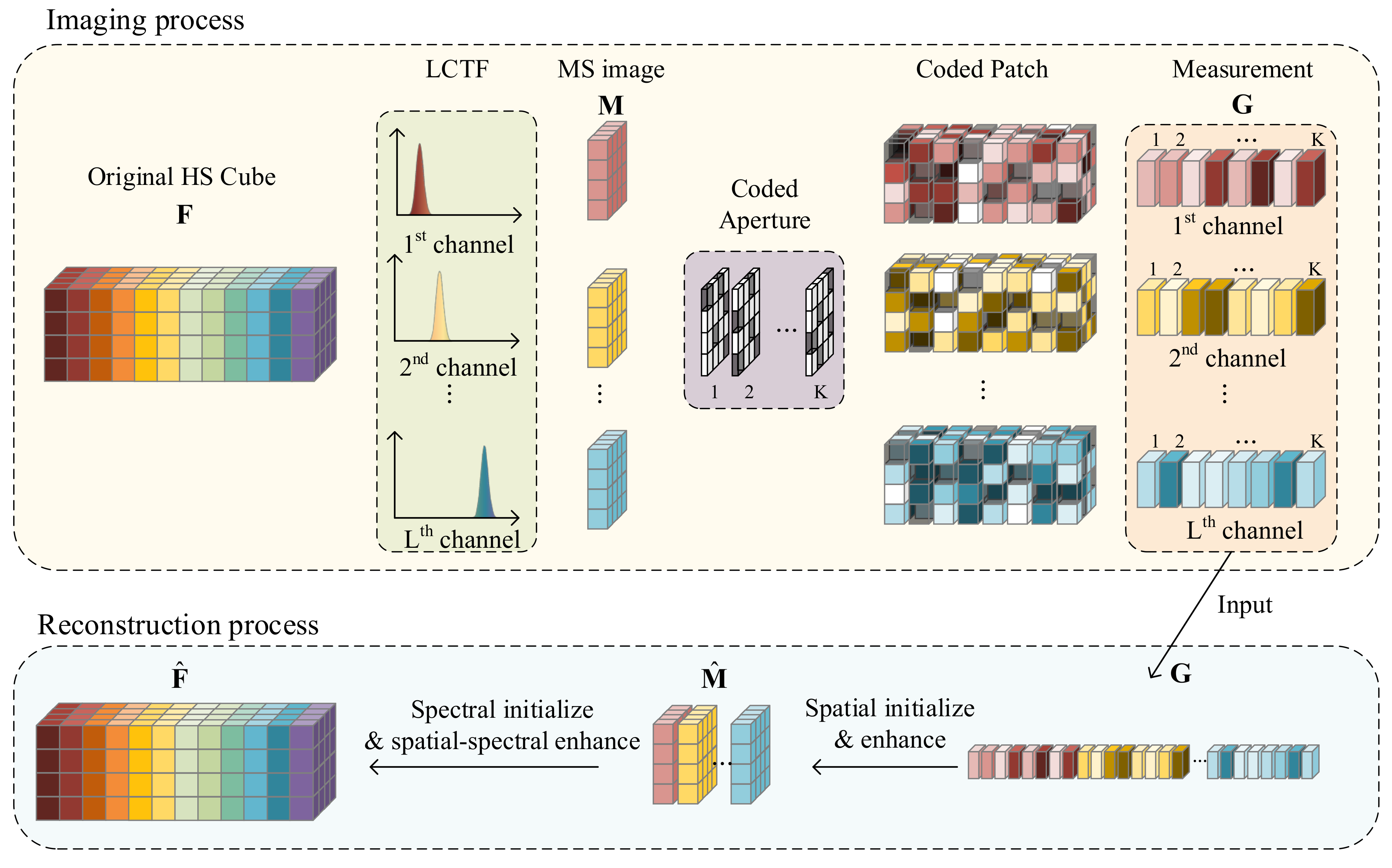
2. CATF Spectral Imager

Figure 1 shows the schematic of CATF spectral imager with its optical structure presented in the dashed box. The reflected light source from the object is modulated by LCTF and DMD, in turn, and received by the detector. Concretely, the imaging lens first focuses the reflected light on LCTF that modulates the object’s spectral information by adjusting the amplitudes of selected channel transmission functions. The spectrally modulated scene is then imaged on the DMD by the first relay lens to undergo spatially modulation with a random coded aperture pattern. Finally, the compressed measurements are projected on the detector by the second relay lens.

Differently from traditional imaging systems, the detector hereby receives compressed measurements that need to be further reconstructed by algorithms to obtain final HS images. The original HS cube is denoted by $\mathbf{F}\in {\mathbb{R}}^{N_{\lambda }\times N_x\times N_y}$ with a spatial resolution of $N_x\times N_y$ and $N_{\lambda }$ number of spectral bands. Multiple sampling in both spectral and spatial dimensions is required to achieve accurate HS data reconstruction. Let L denote the spectral sampling number (i.e., the number of LCTF channels) and K denote the spatial sampling number (i.e., the number of coded patterns in the DMD). Then, the compressed measurements acquired on the detector can be expressed as $\mathbf{G}\in {\mathbb{R}}^{L\times K\times M_x\times M_y}$, where $M_x\times M_y$ denotes the dimension of the detector. Since the spatial resolution of the detector is usually much smaller than that of the coded aperture, the scaling factor is $R=N_x/M_x=N_y/M_y$. Note that we hereby only consider the case where the coded aperture matches with the detector, i.e., R shall be an integer.

Mathematically, let $\mathit{f}\in {\mathbb{R}}^{N_{\lambda }{N}_x{N}_y}$ denote the vectorized representation of the original HS cube, the process of obtaining vectorized compressed measurements $\mathit{g}\in {\mathbb{R}}^{LK{M}_x{M}_y}$ by the detector can be formulated as:

$$\mathit{g}=\mathsf{\Phi }\mathit{f},$$

(1)

where $\mathsf{\Phi }\in {\mathbb{R}}^{LK{M}_x{M}_y\times N_{\lambda }{N}_x{N}_y}$ is the measurement matrix of the system, which can be regarded as the product of a spectral and a spatial measurement matrix determined by the transmission functions of the LCTF and the patterns of the coded aperture, respectively.

The massive information contained in HS image, which inevitably results in high computational cost for reconstruction, poses a great challenge to reconstruct the whole HS images using either iterative algorithms or deep networks. Hence, we adopt a block-compressed sensing (BCS) framework [41] to alleviate computational complexity. Assume that the original HS cube is spatially divided into several $N_{\lambda }\times B\times B$-sized subcubes, each of which corresponds to a $M^B\times M^B$-sized region on the detector ($M^B=B/R$). The measurement matrix of CATF spectral imager can be denoted as:

$$\mathsf{\Phi }=\left[\begin{array}{cccc}{\mathsf{\Phi }}^B& & & \\ & {\mathsf{\Phi }}^B& & \\ & & \ddots & \\ & & & {\mathsf{\Phi }}^B\end{array}\right],$$

(2)

where ${\mathsf{\Phi }}^B$ is the measurement matrix for each subcube, which can be written in the following Kronecker production form:

$${\mathsf{\Phi }}^B={\mathsf{\Phi }}_{\lambda }\otimes {\mathsf{\Phi }}_{xy}^B\in {\mathbb{R}}^{LK{M}^B{M}^B\times N_{\lambda }BB},$$

(3)

where ${\mathsf{\Phi }}_{\lambda }\in {\mathbb{R}}^{L\times N_{\lambda }}$ and ${\mathsf{\Phi }}_{xy}^B\in {\mathbb{R}}^{K{M}^B{M}^B\times BB}$ are the spectral and the spatial measurement matrix for the subcube, respectively. Based on the above analysis, Equation (1) can be decomposed into a number of subproblems:

$${\mathit{g}}^B={\mathsf{\Phi }}^B{\mathit{f}}^B,$$

(4)

where ${\mathit{g}}^B\in {\mathbb{R}}^{LK{M}^B{M}^B}$ are the vectorized compressed measurements for subcube ${\mathit{f}}^B\in {\mathbb{R}}^{N_{\lambda }BB}$. The iterative reconstruction algorithms rely on the sparsity of HS images and thus transform the solution to Equation (4), to an optimization problem of $l_1$ norm:

$$\widehat{{\mathbf{\theta }}^B}=\arg \underset{{\mathit{\theta }}^B}{\min }{∥{\mathit{\theta }}^B∥}_1\mathrm{subject}\mathrm{to}{∥{\mathit{g}}^B-{\mathsf{\Phi }}^B{\mathsf{\Psi }}^B{\mathit{\theta }}^B∥}_2⩽\epsilon ,$$

(5)

where ${\mathsf{\Psi }}^B\in {\mathbb{R}}^{N_{\lambda }BB\times N_{\lambda }BB}$ is the sparse basis of the sub-HS cube, ${\mathbf{\theta }}^B\in {\mathbb{R}}^{N_{\lambda }BB}$ is the sparse coefficient vector, and $\epsilon$ is the reconstruction error bound.

In addition, Equation (4) can also be solved as a total variation (TV) minimization problem:

$${\mathit{f}}^B=\arg \underset{{\mathit{f}}^B}{\min }∥\mathrm{TV}\left({\mathit{f}}^B\right)∥\mathrm{subject}\mathrm{to}{\mathit{g}}^B={\mathsf{\Phi }}^B{\mathit{f}}^B,$$

(6)

where $∥\mathrm{TV}\left({\mathit{f}}^B\right)∥$ denotes the TV norm of ${\mathit{f}}^B$.

3. Methodology

In this section, we first briefly describe design inspiration and representation for network-based reconstruction, and then elaborate on the design of the proposed BTR-Net. The BCS framework is also used in the design of BTR-Net, and the superscript B is omitted for simplicity of writing.

3.1. Design Inspiration and Representation

The intention of the proposed reconstruction network is to reverse the imaging process of spectral imager step by step. Figure 2 illustrates the overall workflow of BTR-Net with the example of acquiring and reconstructing compressed one-pixel measurements on the detector.

For the acquisition process, the input HS subcube $\mathbf{F}\in {\mathbb{R}}^{N_{\lambda }\times B\times B}$, with a spatial resolution of $B\times B$ and $N_{\lambda }$ spectral bands, is first spectrally modulated by LCTF with L channels to produce a multispectral (MS) image $\mathbf{M}\in {\mathbb{R}}^{L\times B\times B}$. The MS image is further spatially encoded by DMD with K different coding patterns to obtain shrunken measurements on an $M^B\times M^B$-sized detector, resulting in modulated output $\mathbf{G}\in {\mathbb{R}}^{(L\times K)\times M^B\times M^B}$.

Conversely, the reconstruction process aims to learn a reverse mapping function $\Theta :\mathbf{G}\to \mathbf{M}\to \mathbf{F}$. It first maps the compressed measurement, $\mathbf{G}$, to an MS image, $\mathbf{M}$, by spanning spatial resolution (spatial initialization) and enriching fine-grained details (spatial enhancement), then it extends its spectral resolution (spectral initialization) and jointly promotes the image quality spatially and spectrally (spatial–spectral enhancement), leading to final reconstructed result $\mathbf{F}$.

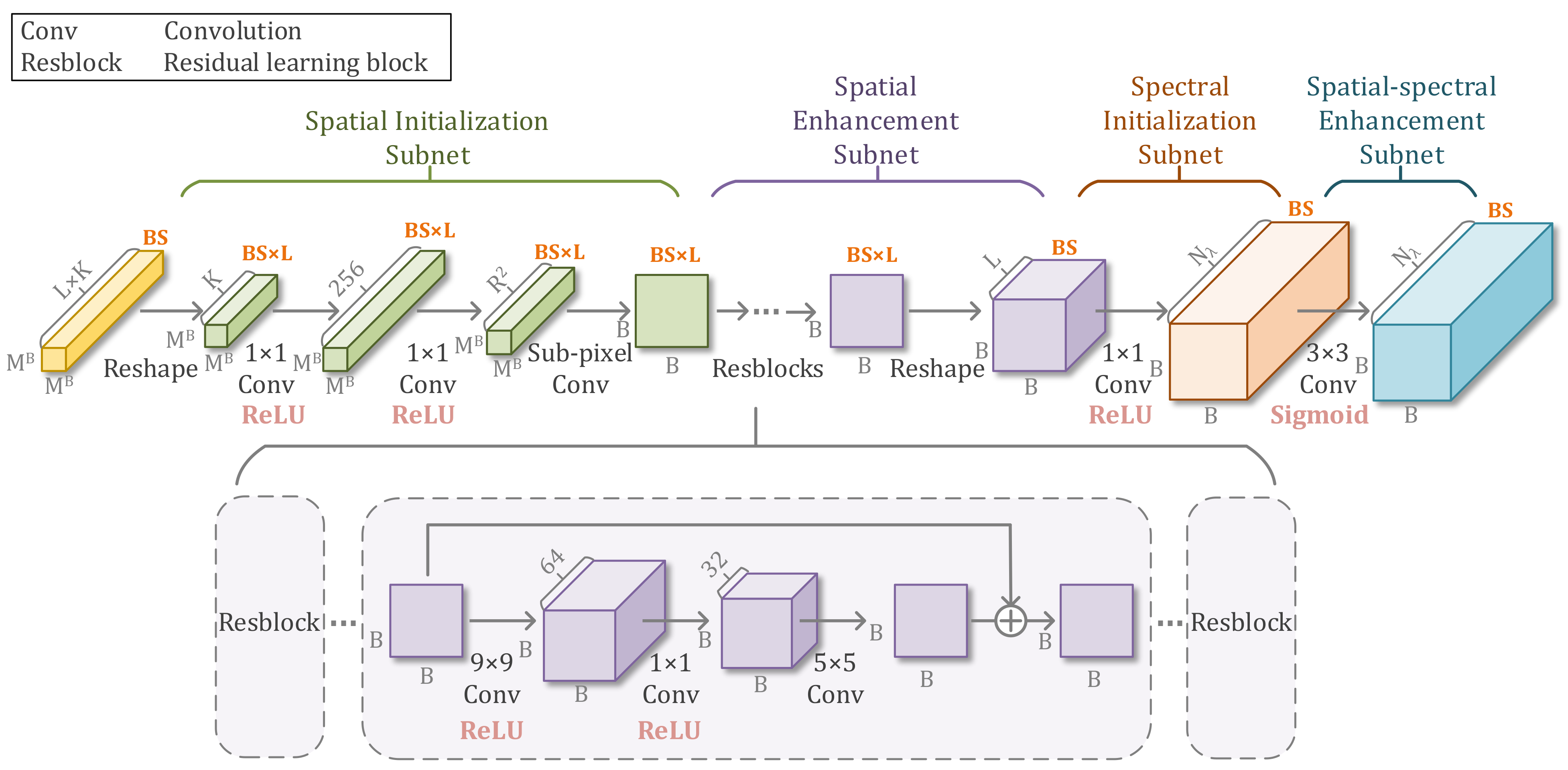
3.2. BTR-Net Architecture

Figure 3 shows the network architecture of the proposed BTR-Net. It is composed of four subnetworks: spatial initialization, spatial enhancement, spectral initialization, and spatial–spectral enhancement subnet, mapping the compressed measurement to original HS data step by step in an interpretable and unified manner. In the following, we use $[\mathrm{batch}\mathrm{size},\mathrm{channel},\mathrm{high},\mathrm{width}]$ to denote the data size in the BTR-Net.

Spatial Initialization Subnet: This aims to acquire the spatial initialization $\widehat{\mathbf{M}}$ from compressed measurement $\mathbf{G}$ by spanning spatial resolution. The function of this subnet can be formulated as follows:

$$\widehat{\mathbf{M}}=\mathcal{P}\mathcal{S}\left(\gamma \left({\mathbf{W}}_2\gamma \left({\mathbf{W}}_1{\mathcal{R}}_1\left(\mathbf{G}\right)\right)\right)\right),$$

(7)

where ${\mathcal{R}}_1$ represents a reshape operation, ${\mathbf{W}}_1$ and ${\mathbf{W}}_2$ are the weights to be trained for the first and second convolution layers, respectively, and each convolution layer is followed by a ReLU activation $\gamma$. $\mathcal{P}\mathcal{S}$ is a periodic shuffling operator called sub-pixel convolution layer, which was first introduced in [30]. More specifically, ${\mathcal{R}}_1$ merges the spectral measurements of the input data g into the batch size dimension (i.e.,$[BS,L\times K,M^B,M^B]\to [BS\times L,K,M^B,M^B]$), thus we were able to focus on the spatial information in the following operations. Subsequent convolutional layers extract features with low spatial resolution, and ensure that the number of feature maps feeding to $\mathcal{P}\mathcal{S}$ is $R^2$ (where $R=B/M^B$). Finally, $\mathcal{PS}$ rearranges $R^2$ features with resolution $M^B\times M^B$ to a single image: $B\times B$ (i.e., $[BS\times L,R^2,M^B,M^B]\to [BS\times L,1,B,B]$).

Spatial Enhancement Subnet: Designed to obtain predicted MS image ${\mathbf{M}}^{\ast }$ from the spatial initialization $\widehat{\mathbf{M}}$ by feature refinement. Mathematically, it learns the following function:

$${\mathbf{M}}^{\ast }={\mathcal{R}}_2\left(\mathcal{H}\left(\widehat{\mathbf{M}},\left\{{\mathcal{F}}_{N_r}\right\}\right)\right),$$

(8)

where ${\mathcal{R}}_2$ performs a reverse operation of ${\mathcal{R}}_1$ (i.e., $[BS\times L,1,B,B]\to [BS,L,B,B]$). $\mathcal{H}$ takes the spatial initialization $\widehat{\mathbf{M}}$ as input and contains $N_r$ residual learning block (Resblock) to be learned. The nth Resblock is defined as:

$${\mathbf{M}}^{n\ast }=\left\{\begin{array}{c}{\mathcal{F}}_n\left(\widehat{\mathbf{M}},\left\{{\mathbf{W}}_i^n\right\}\right)+\widehat{\mathbf{M}},n=1\\ {\mathcal{F}}_n\left({\mathbf{M}}^{\left(n-1\right)\ast },\left\{{\mathbf{W}}_i^n\right\}\right)+{\mathbf{M}}^{\left(n-1\right)\ast },1<n\le N_r\end{array}\right.,$$

(9)

where ${\mathbf{W}}_i^n$ represents the weights to be trained for the ith residual mapping ${\mathcal{F}}_n$. Each Resblock takes the output of the previous Resblock as input and adds the learned residual mapping to the input of the current block as output. The structure of Resblock is designed with reference to the setting in [42], which contains three convolutional layers. The residual mapping is formulated as:

$${\mathcal{F}}_n\left(x,\left\{{\mathbf{W}}_i^n\right\}\right)={\mathbf{W}}_3^r\gamma \left({\mathbf{W}}_2^r\gamma \left({\mathbf{W}}_1^{r}x\right)\right),$$

(10)

where x represents the input, and ${\mathbf{W}}_{{}_i}^r$ is the weight for the ith convolutional layer of residual mapping. Furthermore, the first two convolutional layers are followed by ReLU activation $\gamma$.

Spectral Initialization Subnet: Designed to obtain initialization of the HS image $\widehat{\mathbf{F}}$ via extending the spectral resolution of the predicted MS image ${\mathbf{M}}^{\ast }$, which can be formulated as:

$$\widehat{\mathbf{F}}=\gamma \left({\mathbf{W}}_3{\mathbf{M}}^{\ast }\right),$$

(11)

where ${\mathbf{W}}_3$ represents the weights to be trained. We generated $N_{\lambda }$ feature maps with a convolutional layer to preliminarily reconstruct spectra (i.e., $[BS,L,B,B]\to [BS,N_{\lambda },B,B]$). As with the previous design, an ReLU activation $\gamma$ is added.

Spatial–Spectral Enhancement Subnet: Jointly promotes image quality of the initialized HS image $\widehat{\mathbf{F}}$ spatially and spectrally, resulting in the final reconstructed HS image ${\mathbf{F}}^{\ast }$. The function of this subnet could be expressed as:

$${\mathbf{F}}^{\ast }=\varsigma \left({\mathbf{W}}_4\widehat{\mathbf{F}}\right),$$

(12)

where ${\mathbf{W}}_4$ represents the weights to be trained. Moreover, a Sigmoid activation $\varsigma$ is added to limit the output to between 0 and 1.

It is worth noting that, when we feed the divided images into the network, it is likely to cause distinct block artifacts for the reassemble reconstructed images due to zero-padding. Reflect-padding replaces “zero” with a pixel value at the feature map, so that the convolution result at the edge will not be pulled down. Thus, we use reflect-padding in the padding operation of each convolution layer, which effectively mitigates artifacts caused by block-wise processing [43].

3.3. Loss Function

We optimize the network parameters by minimizing the pixel-wise mean square error (MSE), i.e.,

$$\mathcal{L}\left(\mathsf{\Lambda }\right)=\underset{\mathsf{\Lambda }}{\min }\left\{\frac{1}{N_{\lambda }{B}^2}\sum _{i=1}^{N_{\lambda }}\sum _{j=1}^B\sum _{k=1}^B{\left({\mathbf{F}}_{i,j,k}^{\ast }-{\mathbf{F}}_{i,j,k}\right)}^2\right\},$$

(13)

where $\mathsf{\Lambda }$ is the trainable parameters in BTR-Net, and ${\mathbf{F}}^{\ast }$ and $\mathbf{F}$ represent the HS image predicted by BTR-Net and the original HS image, respectively.

4. Results

We trained the networks from scratch for 30 epochs on a single NVIDIA GeForce GTX 1080, with batch size $BS=10$ and an initial learning rate of ${10}^{-3}$. We gradually decreased the learning rate by an order of magnitude after every 10 epochs. We used two Resblocks in BTR-Net throughout the experiments.

4.1. Dataset and Evaluation Metrics

We carried out experiments on a public HS dataset—the BGU iCVL Hyperspectral Image Dataset [44]. This dataset consists of HS images with 519 spectral bands ranging from 400 to 1000 nm, with a spectral interval of about 1.25 nm. We only used $N_{\lambda }=196$ bands (488 to 730 nm) to make the spectral range of input HS images consistent with that of the LCTF. We randomly selected 32 HS images for training and 8 for testing, and normalized the pixel values of all images to $(0,1)$. Through the blocking operation, more than 12,000 image pairs are used for network training. When generating input data, the following key points should be noted: (i) the original HS images were divided into $196\times 64\times 64$-sized image blocks, and then input cubes of $(22\times 25)\times 8\times 8$ were extracted by spectral filtering and spatial coding; (ii) $L=22$ real measured LCTF transmittance curves were utilized to simulate spectral filtering; and (iii) instead of using the same coded patterns for every image block, $K=25$ random coded patterns (random matrices with values between 0 and 1) were generated for each image block to simulate spatial coding.

For a comprehensive evaluation of the reconstructed results, we adopted mean peak signal to noise ratio (MPSNR), mean structural similarity index measure (MSSIM), mean relative absolute error (MRAE), and mean spectral angle mapper (MSAM) as evaluation metrics. The lower the MRAE and MSAM, or the larger the MSSIM and MPSNR, the better the reconstructed images.

The MPSNR, which measures the difference between two images, is defined as:

$$\mathrm{MPSNR}=\frac{1}{N_{\lambda }}\sum _{i=1}^{N_{\lambda }}10\times {\log }_{10}\left(\frac{1}{{\mathrm{MSE}}_i}\right),$$

(14)

where $N_{\lambda }$ denotes the number of spectral bands, and ${\mathrm{MSE}}_i$ is the MSE between the reconstructed and the original HS image at the ith spectral band.

The MSSIM, which evaluates the structural similarity between the reconstructed and the original images, is defined as:

$$\mathrm{MSSIM}=\frac{1}{N_{\lambda }}\sum _{i=1}^{N_{\lambda }}\frac{\left(2{\mu }_{{\mathbf{F}}_i^{\ast }}{\mu }_{{\mathbf{F}}_i}+c_1\right)\left(2{\sigma }_{{\mathbf{F}}_i^{\ast }{\mathbf{F}}_i}+c_2\right)}{\left({\mu }_{{\mathbf{F}}_i^{\ast }}^2+{\mu }_{{\mathbf{F}}_i}^2+c_1\right)\left({\sigma }_{{\mathbf{F}}_i^{\ast }}^2+{\sigma }_{{\mathbf{F}}_i}^2+c_2\right)},$$

(15)

where ${\mathbf{F}}_i^{\ast }$ (with mean ${\mu }_{{\mathbf{F}}_i^{\ast }}$ and variance ${\sigma }_{{\mathbf{F}}_i^{\ast }}^2$) and ${\mathbf{F}}_i$ (with mean ${\mu }_{{\mathbf{F}}_i}$ and variance ${\sigma }_{{\mathbf{F}}_i}^2$) denote the reconstructed and the original HS image at the ith spectral band, respectively. ${\sigma }_{{\mathbf{F}}_i^{\ast }{\mathbf{F}}_i}$ is the covariance of ${\mathbf{F}}_i^{\ast }$ and ${\mathbf{F}}_i$, and $c_1$ and $c_2$ are the two hyperparameters.

The MRAE, which describes the proportion of the reconstruction error of each pixel to the original value, is defined as:

$$\mathrm{MRAE}=\frac{1}{N_{\lambda }{N}_x{N}_y}\sum _{i=1}^{N_{\lambda }}\sum _{j=1}^{N_x}\sum _{k=1}^{N_y}\frac{\left|{\mathbf{F}}_{i,j,k}^{\ast }-{\mathbf{F}}_{i,j,k}\right|}{{\mathbf{F}}_{i,j,k}},$$

(16)

where ${\mathbf{F}}_{i,j,k}^{\ast }$ and ${\mathbf{F}}_{i,j,k}$ denote the point at the ith spectral band with spatial coordinates of $(j,k)$ on the reconstructed and the original HS image, respectively. $N_x$ and $N_y$ denote the spatial resolution of the HS image.

The MSAM, which calculates the average angle between spectra of the reconstructed and the original images across all spatial positions, is defined as:

$$\mathrm{MSAM}=\frac{1}{N_x{N}_y}{\displaystyle \sum _{j=1}^{N_x}}{\displaystyle \sum _{k=1}^{N_y}}{\cos }^{-1}\frac{{\displaystyle \sum _{i=1}^{N_{\lambda }}}{\mathbf{F}}_{i,j,k}{\mathbf{F}}_{i,j,k}^{\ast }}{\sqrt{{\displaystyle \sum _{i=1}^{N_{\lambda }}}{\left({\mathbf{F}}_{i,j,k}\right)}^2{\displaystyle \sum _{i=1}^{N_{\lambda }}}{\left({\mathbf{F}}_{i,j,k}^{\ast }\right)}^2}}.$$

(17)

4.2. Comparison with Iterative Algorithms

We compare the proposed BTR-Net with popular iterative algorithms, including TwIST [16], GPSR [17], and GAP-TV [18]. TwIST and GPSR aim to find the sparse solution of HS data, as in Equation (5), and the sparse basis is defined as the DCT basis. GAP-TV is a TV-based algorithm.

Table 1. Comparisons of reconstructed quality of BTR-Net and iterative algorithms. Each HS image is with a spatial resolution of $1280\times 1280$ and 196 spectral bands. We adopted mean peak signal to noise ratio (MPSNR), mean structural similarity index measure (MSSIM), mean relative absolute error (MRAE), and mean spectral angle mapper (MSAM) as evaluation metrics.

Methods	Metrics	Scene 1	Scene 2	Scene 3	Scene 4	Scene 5	Scene 6	Scene 7	Scene 8	Average
TwIST	MPSNR	25.9461	25.3603	29.0709	26.4064	25.9091	23.3570	25.3866	25.7167	25.8941
	MSSIM	0.7651	0.7555	0.8446	0.7913	0.7389	0.5745	0.7795	0.7741	0.7529
	MRAE	0.1440	0.1618	0.1548	0.1531	0.1400	0.1304	0.1730	0.1696	0.1533
	MSAM	0.1925	0.1779	0.3029	0.1903	0.1701	0.1683	0.2730	0.3021	0.2221
GPSR	MPSNR	27.7491	26.6125	30.9366	28.0081	28.1142	25.4694	26.6935	27.0328	27.5770
	MSSIM	0.8587	0.8359	0.9056	0.8754	0.8525	0.7100	0.8544	0.8451	0.8422
	MRAE	0.1012	0.1294	0.1106	0.1130	0.1018	0.1053	0.1312	0.1358	0.1160
	MSAM	0.1473	0.1422	0.2434	0.1415	0.1341	0.1469	0.2113	0.2525	0.1774
GAP-TV	MPSNR	27.0290	26.0617	29.6778	27.3291	27.1311	26.1558	25.3088	25.8458	26.8174
	MSSIM	0.8977	0.8728	0.9032	0.8977	0.8959	0.9187	0.8442	0.8459	0.8845
	MRAE	0.1445	0.1582	0.1781	0.1526	0.1368	0.1230	0.1959	0.1920	0.1601
	MSAM	0.2090	0.1938	0.3237	0.2079	0.1861	0.1830	0.2947	0.3230	0.2402
BTR-Net	MPSNR	31.4361	29.2063	35.0696	30.2514	32.4901	33.7753	30.2386	29.9614	31.5536
	MSSIM	0.9354	0.9065	0.9682	0.9242	0.9356	0.9485	0.9160	0.9009	0.9294
	MRAE	0.0473	0.0786	0.0544	0.0679	0.0454	0.0254	0.0724	0.0780	0.0587
	MSAM	0.0257	0.0337	0.0458	0.0316	0.0225	0.0199	0.0371	0.0491	0.0332

provides quantitative comparisons of reconstructed results from our BTR-Net and iterative algorithms. One can see that BTR-Net outperforms the three iterative algorithms in terms of all three metrics on each testing image (without noise). For instance, BTR-Net gains more than 4 dB over iterative algorithms in terms of average MPSNR.

Table 2. Comparisons of running time (average time to reconstruct an HS image with a spatial resolution of $1280\times 1280$ and 196 spectral bands).

Methods	TwIST	GPSR	GAP-TV	BTR-Net
Running time(s) CPU/GPU	$1.35\times {10}^4/$–	$1.15\times {10}^4/$–	$1.08\times {10}^4/$–	$1.29\times {10}^2/3.36$

shows the running time required for each methods to reconstruct an HS image with a spatial resolution of $1280\times 1280$ and 196 spectral bands. BTR-Net demonstrates significant decrease in running time compared with iterative algorithms. Specifically, BTR-Net runs two orders of magnitude faster than iterative algorithms on CPU. Moreover, BTR-Net supports acceleration using GPU, which makes it runs about 38 times faster than when using CPU.

Figure 4 shows qualitative comparisons of the reconstructed results in RGB projection. The red, green and blue channels of the RGB image are taken from three spectral bands of the HS image at 660 nm, 550 nm and 500 nm, respectively. For a clear comparison of reconstructed details, the image region in red square is enlarged at the lower left corner of the RGB image. The RGB images indicate that BTR-Net is superior to conventional iterative algorithms in color reproduction and detail recovery.

Figure 5 compares spectral curves reconstructed by these four methods. The second and third columns draw the spectra of two representative pixels whose positions are marked on the RGB image in the first column, where the x-axis and y-axis represent wavelength and normalized intensity, respectively. The SAM is labeled in the legend to evaluate the quality of the reconstructed spectra. The spectra suggest that BTR-Net performs well in spectrum reconstruction, while conventional iterative algorithms show poor performance at the edge of spectrum.

In order to further demonstrate the wavelength-dependent performance variation, we quantitatively compare the results at different wavelengths (taking Scene 1 as an example), as shown in Figure 6. One can see that the proposed BTR-Net possesses excellent global performance and stable reconstructed outcomes. By comparison, the reconstructed results of iterative algorithms change significantly with wavelength, probably due to the fact that the spectra are not strictly sparse on the given sparse basis.

We studied the noise immunity of BTR-Net by adding white Gaussian noise to the compressive measurements (i.e., input data of BTR-Net). The network is trained in the absence of noise and tested in the presence of noise. The three iterative algorithms were also tested by adding noise to the compressive measurements.

Table 3. Performance of different noise level (average of all test images).

Methods	Metrics	None	40 dB	30 dB	20 dB
TwIST	MPSNR	25.8941	25.2734	22.7043	15.9897
	MSSIM	0.7529	0.7225	0.5942	0.2820
	MRAE	0.1533	0.1625	0.2048	0.4066
	MSAM	0.2221	0.2277	0.2617	0.4585
GPSR	MPSNR	27.5770	27.4652	25.8821	12.0305
	MSSIM	0.8422	0.8385	0.7816	0.1633
	MRAE	0.1160	0.1175	0.1245	0.5493
	MSAM	0.1774	0.1779	0.1893	0.6204
GAP-TV	MPSNR	26.8174	26.6058	25.3251	20.5241
	MSSIM	0.8845	0.8736	0.8011	0.5357
	MRAE	0.1601	0.1755	0.1889	0.2654
	MSAM	0.2402	0.2418	0.2512	0.3299
BTR-Net	MPSNR	31.5536	31.5209	31.3158	29.9170
	MSSIM	0.9294	0.9294	0.9292	0.9278
	MRAE	0.0587	0.0594	0.0625	0.0820
	MSAM	0.0332	0.0332	0.0332	0.0334

compares the experimental results with noise levels of 40 dB, 30 dB and 20 dB. Taking Scene 1 as an example, Figure 7 compares the visual quality of these four methods at different noise levels, and Figure 8 shows the performance of the reconstructed spectra. It can be observed that the proposed BTR-Net surpasses iterative algorithms in terms of reconstruction performance and anti-noise ability. Concretely, the results of BTR-Net are almost impervious to the addition of 40 dB and 30 dB noise; although the 20 dB noise slows down the performance of BTR-Net, it is still acceptable. By contrast, the performance of TwIST declines obviously with 30 dB noise; the performance of GPSR and GAP-TV degrades but is still acceptable. When the noise level is set to 20 dB, TwIST and GPSR can hardly reconstruct the data successfully; the noise immunity of GAP-TV is better than that of TwIST and GPSR, but the reconstruction result is unsatisfactory with 20 dB noise.

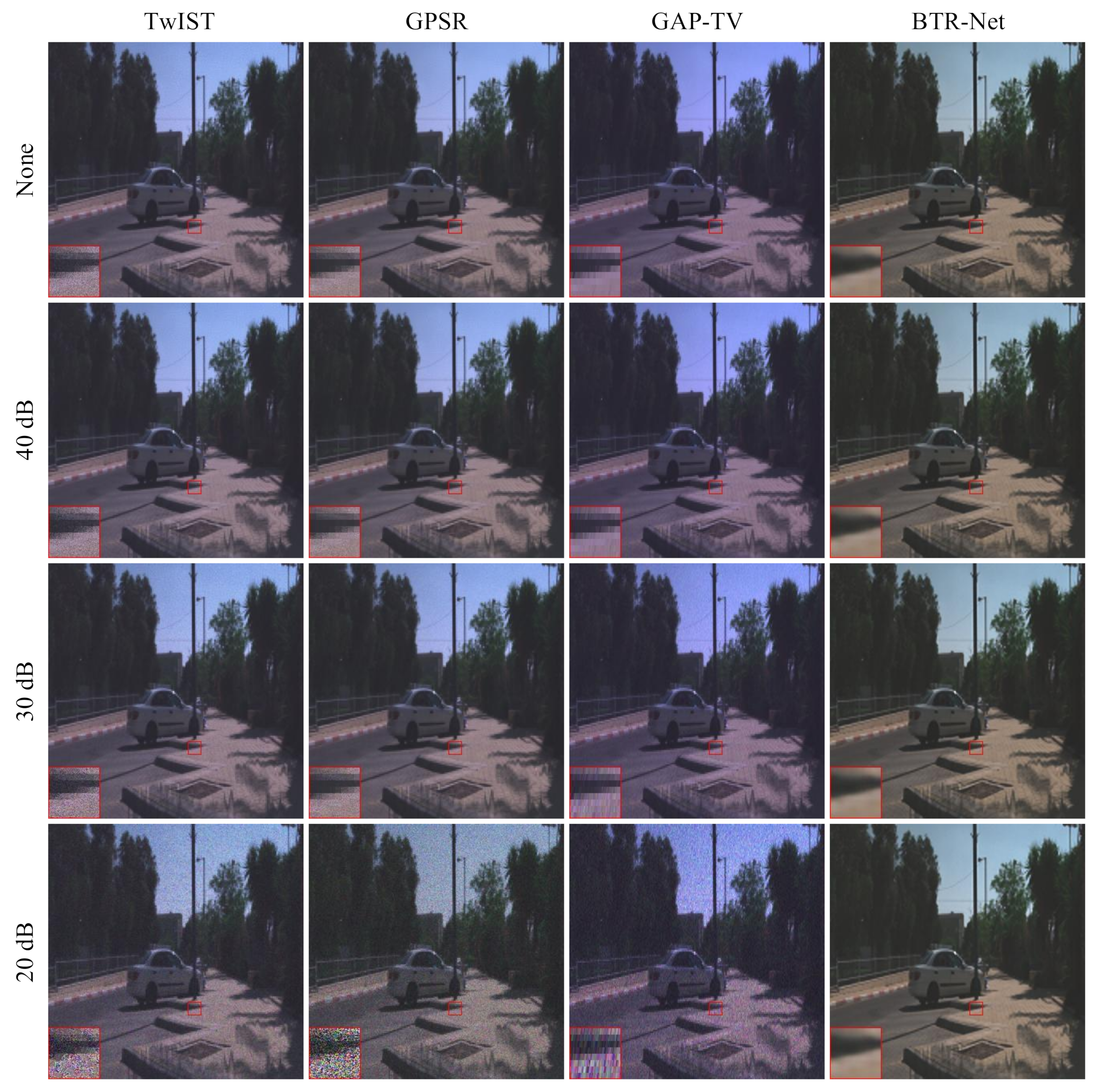
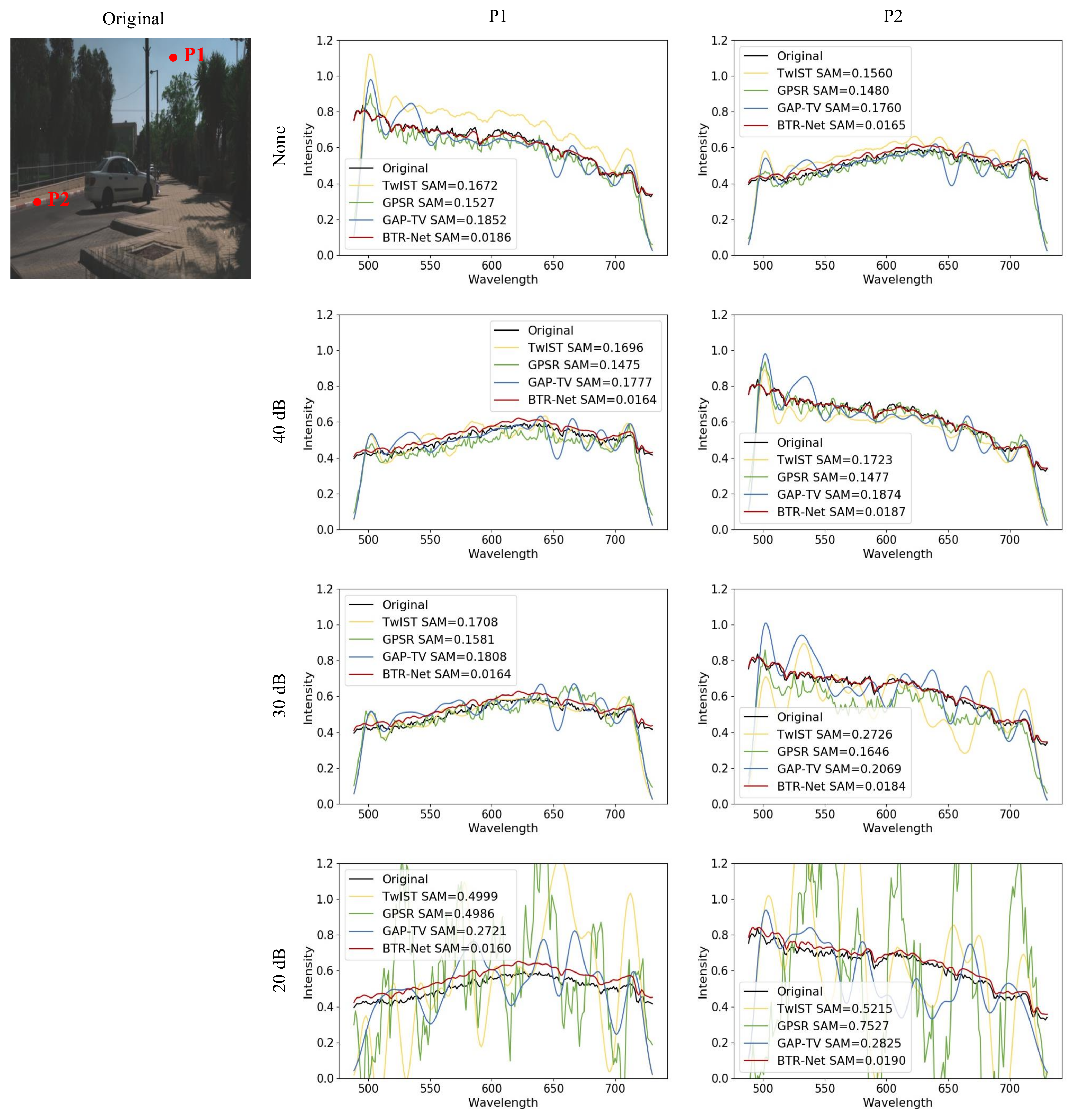
4.3. Real Experiments

We constructed an experimental prototype of the CATF spectral imager, as shown in Figure 9. The testbed consisted of a fiber ring illuminator (Thorlabs FRI61F50 and OSL2), an imaging lens with a focal length of 50 mm, a visible LCTF with a range of 500 nm–710 nm, two relay lenses with a focal length of 75 mm, a DMD (Texas Instruments DLP9500), and a monochromatic CMOS camera (Basler acA2040-90 um).

We took a set of compressive measurements by the prototype as the input data of the trained BTR-Net. Consistent with the parameter settings in simulations, $L=22$ LCTF channels and $K=25$ random coded patterns were taken in real experiments, and the scaling factor was set to $R=8$. The object occupied $384\times 384$ pixels on the DMD, which corresponded to $48\times 48$ pixels on the detector. The measurements were spatially divided into $8\times 8$ image blocks to meet the requirements of the BTR-Net on the size of input data.

In real experiments, we used the CATF spectral imager to obtain the measurements, but could not obtain the ground truth of the corresponding HS data. This made it impossible to train the BTR-Net with the dataset obtained in real experiments. So, we applied the trained BTR-Net in simulations to the real experiment. This was challenging since our BTR-Net was not trained with real data and the performance of the measurement matrix in the real experiments was degraded compared with the matrix used to generate the training data.

To compare the results qualitatively, Figure 10 shows the RGB projections of the reconstructed results from the real experimental data, including three iterative algorithms and the proposed BTR-Net. It can be seen that the colors of the RGB images are similar, which reflects that the spectral reconstruction capabilities of the four methods are comparable. Perceptually, the BTR-Net is superior to iterative algorithms in detail recovery.

Figure 11 draws the reflection spectra of two representative points whose positions are marked on the RGB image, where the x-axis and y-axis represent wavelength and reflectivity, respectively. The PSNR is labeled in the legend to evaluate the quality of the reconstructed spectra. The original reflection spectra are measured by a grating spectrometer (Ocean Optics Maya2000pro). The result shows that the reconstructed spectra of BTR-Net is in the best agreement with the original spectra in P1. These four methods show comparable spectral reconstruction performance at the background P2.

In real experiments, iterative algorithms tend to obtain a solution with high sparsity in order to combat noise (that is, the number of non-zero coefficients of ${\theta }^B$ in Equation (5) is extremely small). The reconstructed results of iterative algorithms lose a large proportion of high-frequency components, resulting in a lack of spatial details and relatively smooth spectra. Our BTR-Net learned the characteristics of HS dataset in the training. Thus, the details in the RGB projections were richer, and the spectra contained more fluctuations. The results demonstrate the feasibility of the proposed BTR-Net; although, the results are not as good as in the simulation.

5. Discussion

In this section, We further discuss our design choices and parameter settings in the proposed BTR-Net.

5.1. Effect of Up-Sampling Methods

We adopt sub-pixel convolution to up-sample low-resolution measurements in spatial initialization subnet. To validate our design, we compared it with the model variant by replacing sub-pixel convolution with an alternative up-sampling approach, i.e., bilinear interpolation. Figure 12 and

Table 4. Quantitative comparisons of using sub-pixel convolution and bilinear interpolation (the metric is the average of all test images).

Methods	MPSNR(dB)	MSSIM	MRAE	MSAM
Sub-pixel Convolution	31.5536	0.9294	0.0586	0.0332
Bilinear Interpolation	30.6836	0.9226	0.0706	0.0362

depict training error curve and quantitative comparisons of the reconstructed results, respectively. The model with either up-sampling approach can converge quickly, demonstrating the universality and rationality of our network design. Furthermore, the model with sub-pixel convolution achieves lower training error and better quantitative results, showing its superiority in enlarging spatial resolutions while retaining beneficial local structures.

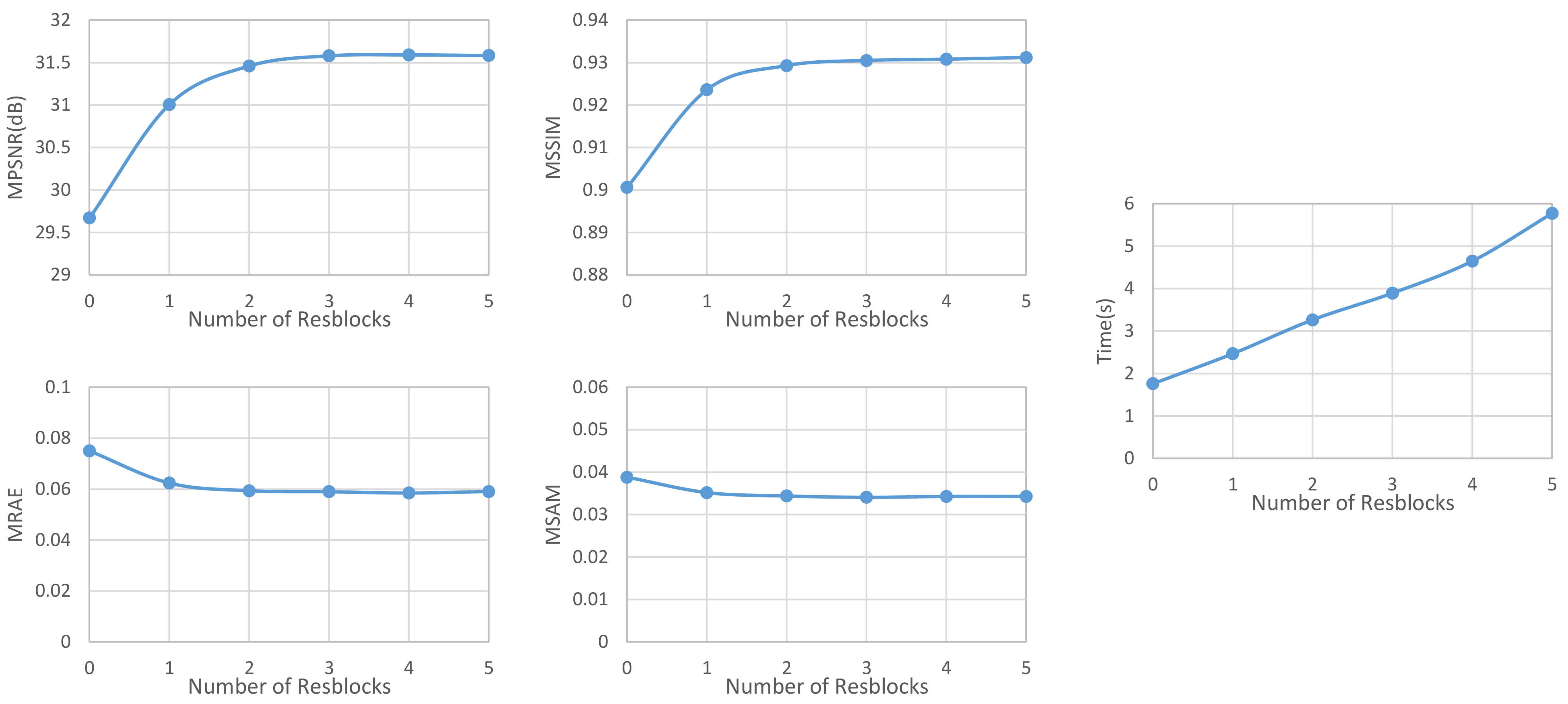
5.2. Effect of Resblock Number

The Resblock infers the residual between spatial initialized image and MS image, thereby ameliorating image quality. We test the effect of incorporating different numbers of Resblock in the spatial enhancement subnet. Figure 13 presents the varying trend of reconstruction quality and running speed with an increasing number of Resblocks. Generally, incorporating more Resblocks brings higher reconstruction quality, but at the cost of decreasing the running speed. We observe that reconstruction quality improves as the block number $N_r$ increases; however, the curves are almost flat when $N_r\ge 4$. Considering the tradeoff between network complexity and reconstruction performance, we set the default block number $N_r=2$ for BTR-Net. It is worth noting that BTR-Net performed better than iterative algorithms even without using any Resblocks for feature refinement, evidencing the effectiveness of backtracking reconstruction strategy itself.

5.3. Effect of Kernel Size in Resblock

Each Resblock in the spatial enhancement subnet contains three convolutional layers with different kernel sizes $K_s$ to extract multiscale features. The Resblock in DR2-Net [42], which we borrowed from, applies a combination of relatively large kernel sizes, i.e., $K_s$ = 11-1-7, resulting in added computation. To balance complexity and reconstruction performance, we test the model with shrunken convolutional kernels in Resblock.

Table 5. Performance and time complexity of using different kernel sizes in Resblock (the metric is the average of all test images).

Kernel Size	MPSNR(dB)	MSSIM	MRAE	MSAM	Time Complexity
11-1-7	31.6100	0.9302	0.0585	0.0333	$\sim 4.6\times {10}^7$
9-1-5	31.5536	0.9294	0.0586	0.0332	$\sim 3.3\times {10}^7$
7-1-3	31.3566	0.9269	0.0605	0.0332	$\sim 2.2\times {10}^7$

lists the quantitative comparisons of reconstructed results in $K_s$ = 11-1-7, 9-1-5 and 7-1-3, and the time complexity of one Resblock with different parameter settings. Diminution in kernel size degrades the reconstruction performance, while bringing the benefit of reducing the time and complexity. To weigh gains and losses, we set the parameter to $K_s$ = 9-1-5 for our Resblock.

5.4. Cross-Validation

We perform K-fold cross-validation experiments to verify the performance of the proposed BTR-Net. The original HS images are randomly divided into 5 groups, each of which contains 8 HS images. In each experiment, we selected one group as the testing set, and the other groups as the training set. Through the blocking operation, more than 12,000 image pairs are used for training in each experiment. The cross-validation process is repeat 5 times, and the results are shown in

Table 6. Cross-validation of BTR-Net.

Testing Set	MPSNR	MSSIM	MRAE	MSAM
1	30.9160	0.9173	0.0563	0.0316
2	30.8934	0.9116	0.0589	0.0315
3	30.9825	0.9136	0.0568	0.0327
4	31.6278	0.9209	0.0518	0.0289
5	31.5536	0.9294	0.0587	0.0332
Average	31.1947	0.9186	0.0565	0.0316

. The results show that the proposed BTR-Net is reliable and stable.

6. Conclusions

Suffering from traditional, iteration-based algorithms, we propose a backtracking reconstruction network called BTR-Net to solve the reconstruction problem in three-dimensional compressed HS imaging. We decomposed the imaging process based on CATF spectral imager into steps, and designed a series of subnetworks to reverse these steps. Specifically, we built four subnetworks—spatial initialization subnet, spatial enhancement subnet, spectral initialization subnet, and spatial–spectral enhancement subnet—in sequence, to obtain a reverse mapping from compressed measurements to HS data. Experimental results show that the proposed BTR-Net outperforms traditional iteration-based algorithms in reconstruction performance and running speed, while exhibiting great noise resistance.

The BTR-Net shows obvious advantages over iterative algorithms, yet there are several aspects requiring further study:

1. Multiple reshaping operations were adopted in BTR-Net, which means that the size of input data needs to be strictly limited once the network is trained. Follow-up work will be directed towards the design of a fully convolutional network capable of accepting variable dimension input data.

2. The BTR-Net takes compressed measurements as inputs to reconstruct HS data, which ignores characteristics of the imaging system itself, such as the transmittance curves of LCTF and coded patterns of DMD. Further effort is needed to design a network that rationally utilizes these prior information to make the network more interpretable.

References

1. Zhang, B.; Wu, D.; Zhang, L.; Jiao, Q.; Li, Q. Application of hyperspectral remote sensing for environment monitoring in mining areas. Environ. Earth Sci. 2012, 65, 649–658. [Google Scholar] [CrossRef]
2. Roberts, D.A.; Quattrochi, D.A.; Hulley, G.C.; Hook, S.J.; Green, R.O. Synergies between VSWIR and TIR data for the urban environment: An evaluation of the potential for the Hyperspectral Infrared Imager (HyspIRI) Decadal Survey mission. Remote Sens. Environ. 2012, 117, 83–101. [Google Scholar] [CrossRef]
3. Li, W.; Du, Q. A survey on representation-based classification and detection in hyperspectral remote sensing imagery. Pattern Recognit. Lett. 2016, 83, 115–123. [Google Scholar] [CrossRef]
4. Jay, S.; Guillaume, M.; Minghelli, A.; Deville, Y.; Chami, M.; Lafrance, B.; Serfaty, V. Hyperspectral remote sensing of shallow waters: Considering environmental noise and bottom intra-class variability for modeling and inversion of water reflectance. Remote Sens. Environ. 2017, 200, 352–367. [Google Scholar] [CrossRef]
5. Yu, C.; Yang, J.; Song, N.; Sun, C.; Wang, M.; Feng, S. Microlens array snapshot hyperspectral microscopy system for the biomedical domain. Appl. Opt. 2021, 60, 1896–1902. [Google Scholar] [CrossRef]
6. Donoho, D. Compressed sensing. IEEE Trans. Inf. Theory 2006, 52, 1289–1306. [Google Scholar] [CrossRef]
7. Neifeld, M.A.; Ke, J. Optical architectures for compressive imaging. Appl. Opt. 2007, 46, 5293–5303. [Google Scholar] [CrossRef] [PubMed]
8. Duarte, M.F.; Davenport, M.A.; Takhar, D.; Laska, J.N.; Sun, T.; Kelly, K.F.; Baraniuk, R.G. Single-pixel imaging via compressive sampling. IEEE Signal Process. Mag. 2008, 25, 83–91. [Google Scholar] [CrossRef] [Green Version]
9. Wagadarikar, A.; John, R.; Willett, R.; Brady, D. Single disperser design for coded aperture snapshot spectral imaging. Appl. Opt. 2008, 47, B44. [Google Scholar] [CrossRef] [Green Version]
10. Lin, X.; Liu, Y.; Wu, J.; Dai, Q. Spatial-spectral encoded compressive hyperspectral imaging. ACM Trans. Graph. 2014, 33, 1–11. [Google Scholar] [CrossRef]
11. Wang, L.; Xiong, Z.; Shi, G.; Wu, F.; Zeng, W. Adaptive Nonlocal Sparse Representation for Dual-Camera Compressive Hyperspectral Imaging. IEEE Trans. Pattern Anal. Mach. Intell. 2017, 39, 2104–2111. [Google Scholar] [CrossRef]
12. Ren, W.; Fu, C.; Wu, D.; Xie, Y.; Arce, G.R. Channeled compressive imaging spectropolarimeter. Opt. Express 2019, 27, 2197–2211. [Google Scholar] [CrossRef]
13. Wang, X.; Zhang, Y.; Ma, X.; Xu, T.; Arce, G.R. Compressive spectral imaging system based on liquid crystal tunable filter. Opt. Express 2018, 26, 25226–25243. [Google Scholar] [CrossRef]
14. Zhang, Y.; Xu, T.; Wang, X.; Pan, C.; Hao, J.; Huang, C. Real-time adaptive coded aperture: Application to the compressive spectral imaging system. In Proceedings of the Optics, Photonics and Digital Technologies for Imaging Applications VI, Online, 6–10 April 2020; Schelkens, P., Kozacki, T., Eds.; International Society for Optics and Photonics, SPIE: Bellingham, WA, USA, 2020; Volume 11353, pp. 280–289. [Google Scholar]
15. Xu, C.; Xu, T.; Yan, G.; Ma, X.; Zhang, Y.; Wang, X.; Zhao, F.; Arce, G.R. Super-resolution compressive spectral imaging via two-tone adaptive coding. Photon. Res. 2020, 8, 395–411. [Google Scholar] [CrossRef]
16. Bioucas-Dias, J.M.; Figueiredo, M.A.T. A New TwIST: Two-Step Iterative Shrinkage/Thresholding Algorithms for Image Restoration. IEEE Trans. Image Process. 2007, 16, 2992–3004. [Google Scholar] [CrossRef] [Green Version]
17. Figueiredo, M.A.T.; Nowak, R.D.; Wright, S.J. Gradient Projection for Sparse Reconstruction: Application to Compressed Sensing and Other Inverse Problems. IEEE J. Sel. Top. Signal Process. 2007, 1, 586–597. [Google Scholar] [CrossRef] [Green Version]
18. Yuan, X. Generalized alternating projection based total variation minimization for compressive sensing. In Proceedings of the 2016 IEEE International Conference on Image Processing (ICIP), Phoenix, AZ, USA, 25–28 September 2016; pp. 2539–2543. [Google Scholar]
19. Wagadarikar, A.A.; Pitsianis, N.P.; Sun, X.; Brady, D.J. Spectral image estimation for coded aperture snapshot spectral imagers. In Proceedings of the Image Reconstruction from Incomplete Data V, San Francisco, CA, USA, 28 August 2008; International Society for Optics and Photonics, SPIE: Bellingham, WA, USA, 2008; Volume 7076, pp. 9–23. [Google Scholar]
20. Mousavi, A.; Baraniuk, R.G. Learning to invert: Signal recovery via Deep Convolutional Networks. In Proceedings of the 2017 IEEE International Conference on Acoustics, Speech and Signal Processing (ICASSP), New Orleans, LA, USA, 5–9 March 2017; pp. 2272–2276. [Google Scholar]
21. Metzler, C.A.; Maleki, A.; Baraniuk, R.G. From Denoising to Compressed Sensing. IEEE Trans. Inf. Theory 2016, 62, 5117–5144. [Google Scholar] [CrossRef]
22. Wang, L.; Feng, Y.; Gao, Y.; Wang, Z.; He, M. Compressed Sensing Reconstruction of Hyperspectral Images Based on Spectral Unmixing. IEEE J. Sel. Top. Appl. Earth Obs. Remote Sens. 2018, 11, 1266–1284. [Google Scholar] [CrossRef]
23. Xue, J.; Zhao, Y.; Liao, W.; Chan, J.C.W. Nonlocal Tensor Sparse Representation and Low-Rank Regularization for Hyperspectral Image Compressive Sensing Reconstruction. Remote Sens. 2019, 11, 193. [Google Scholar] [CrossRef] [Green Version]
24. Chen, Y.; Huang, T.; He, W.; Yokoya, N.; Zhao, X. Hyperspectral Image Compressive Sensing Reconstruction Using Subspace-Based Nonlocal Tensor Ring Decomposition. IEEE Trans. Image Process. 2020, 29, 6813–6828. [Google Scholar] [CrossRef]
25. Takeyama, S.; Ono, S.; Kumazawa, I. A Constrained Convex Optimization Approach to Hyperspectral Image Restoration with Hybrid Spatio-Spectral Regularization. Remote Sens. 2020, 12, 3541. [Google Scholar] [CrossRef]
26. Schmidhuber, J. Deep learning in neural networks: An overview. Neural Netw. 2015, 61, 85–117. [Google Scholar] [CrossRef] [Green Version]
27. Rastegari, M.; Ordonez, V.; Redmon, J.; Farhadi, A. XNOR-Net: ImageNet Classification Using Binary Convolutional Neural Networks. In Proceedings of the Computer Vision—ECCV 201, 14th European Conference, Amsterdam, The Netherlands, 11–14 October 2016; Leibe, B., Matas, J., Sebe, N., Welling, M., Eds.; Springer International Publishing: Cham, Switzerland, 2016; pp. 525–542. [Google Scholar]
28. Moeskops, P.; Viergever, M.A.; Mendrik, A.M.; de Vries, L.S.; Benders, M.J.N.L.; Išgum, I. Automatic Segmentation of MR Brain Images With a Convolutional Neural Network. IEEE Trans. Med. Imaging 2016, 35, 1252–1261. [Google Scholar] [CrossRef] [Green Version]
29. Liskowski, P.; Krawiec, K. Segmenting Retinal Blood Vessels With Deep Neural Networks. IEEE Trans. Med. Imaging 2016, 35, 2369–2380. [Google Scholar] [CrossRef]
30. Shi, W.; Caballero, J.; Huszár, F.; Totz, J.; Aitken, A.P.; Bishop, R.; Rueckert, D.; Wang, Z. Real-Time Single Image and Video Super-Resolution Using an Efficient Sub-Pixel Convolutional Neural Network. In Proceedings of the 2016 IEEE Conference on Computer Vision and Pattern Recognition (CVPR), Las Vegas, NV, USA, 27–30 June 2016; pp. 1874–1883. [Google Scholar]
31. Chen, L.C.; Papandreou, G.; Kokkinos, I.; Murphy, K.; Yuille, A.L. DeepLab: Semantic Image Segmentation with Deep Convolutional Nets, Atrous Convolution, and Fully Connected CRFs. IEEE Trans. Pattern Anal. Mach. Intell. 2018, 40, 834–848. [Google Scholar] [CrossRef] [PubMed] [Green Version]
32. Li, X.; Zhang, G.; Qiao, H.; Bao, F.; Deng, Y.; Wu, J.; He, Y.; Yun, J.; Lin, X.; Xie, H.; et al. Unsupervised content-preserving transformation for optical microscopy. Light. Sci. Appl. 2021, 10, 44. [Google Scholar] [CrossRef] [PubMed]
33. Zhang, W.; Song, H.; He, X.; Huang, L.; Zhang, X.; Zheng, J.; Shen, W.; Hao, X.; Liu, X. Deeply learned broadband encoding stochastic hyperspectral imaging. Light. Sci. Appl. 2021, 10, 108. [Google Scholar] [CrossRef]
34. Wang, L.; Zhang, T.; Fu, Y.; Huang, H. HyperReconNet: Joint Coded Aperture Optimization and Image Reconstruction for Compressive Hyperspectral Imaging. IEEE Trans. Image Process. 2019, 28, 2257–2270. [Google Scholar] [CrossRef] [PubMed]
35. Miao, X.; Yuan, X.; Pu, Y.; Athitsos, V. lambda-Net: Reconstruct Hyperspectral Images From a Snapshot Measurement. In Proceedings of the 2019 IEEE/CVF International Conference on Computer Vision (ICCV), Seoul, Korea, 27 October–2 November 2019; pp. 4058–4068. [Google Scholar]
36. Wang, L.; Sun, C.; Fu, Y.; Kim, M.H.; Huang, H. Hyperspectral Image Reconstruction Using a Deep Spatial-Spectral Prior. In Proceedings of the 2019 IEEE/CVF Conference on Computer Vision and Pattern Recognition (CVPR), Long Beach, CA, USA, 15–20 June 2019; pp. 8024–8033. [Google Scholar]
37. Wang, L.; Sun, C.; Zhang, M.; Fu, Y.; Huang, H. DNU: Deep Non-Local Unrolling for Computational Spectral Imaging. In Proceedings of the 2020 IEEE/CVF Conference on Computer Vision and Pattern Recognition (CVPR), Seattle, WA, USA, 13–19 June 2020; pp. 1658–1668. [Google Scholar]
38. Yang, Y.; Xie, Y.; Chen, X.; Sun, Y. Hyperspectral Snapshot Compressive Imaging with Non-Local Spatial-Spectral Residual Network. Remote Sens. 2021, 13, 1812. [Google Scholar] [CrossRef]
39. Gedalin, D.; Oiknine, Y.; Stern, A. DeepCubeNet: Reconstruction of spectrally compressive sensed hyperspectral images with deep neural networks. Opt. Express 2019, 27, 35811–35822. [Google Scholar] [CrossRef] [PubMed]
40. He, K.; Zhang, X.; Ren, S.; Sun, J. Deep Residual Learning for Image Recognition. In Proceedings of the 2016 IEEE Conference on Computer Vision and Pattern Recognition (CVPR), Las Vegas, NV, USA, 27–30 June 2016; pp. 770–778. [Google Scholar]
41. Gan, L. Block Compressed Sensing of Natural Images. In Proceedings of the 2007 15th International Conference on Digital Signal Processing, Wales, UK, 1–4 July 2007; pp. 403–406. [Google Scholar]
42. Yao, H.; Dai, F.; Zhang, S.; Zhang, Y.; Tian, Q.; Xu, C. DR2-Net: Deep Residual Reconstruction Network for image compressive sensing. Neurocomputing 2019, 359, 483–493. [Google Scholar] [CrossRef] [Green Version]
43. Alsallakh, B.; Kokhlikyan, N.; Miglani, V.; Yuan, J.; Reblitz-Richardson, O. Mind the Pad–CNNs can Develop Blind Spots. arXiv 2020, arXiv:2010.02178. [Google Scholar]
44. Arad, B.; Ben-Shahar, O. Sparse Recovery of Hyperspectral Signal from Natural RGB Images. In Proceedings of the European Conference on Computer Vision, Amsterdam, The Netherlands, 11–14 October 2016; Springer: Berlin/Heidelberg, Germany, 2016; pp. 19–34. [Google Scholar]
Figure 1. Schematic of coded aperture tunable filter (CATF) spectral imager. The reflected light source from the object is modulated by liquid crystal tunable filter (LCTF) and digital micromirror device (DMD). Each block on the DMD represents a micromirror unit. The micromirror unit in ON state (in white) reflects the light along the main optical axis to the detector, while the unit in OFF state (in black) reflects the light far away from the main optical axis.
Remotesensing 14 02406 g001
Figure 2. The imaging model of the CATF spectral imager and the reconstruction process (diagram of one pixel on the detector). The upper part of the figure describes the imaging process of the CATF spectral imager. The original hyperspectral (HS) cube is first filtered by LCTF with L channels to generate multispectral (MS) image (without loss of spatial resolution). It is then spatially modulated by DMD with K coded apertures. Finally, L × K measurements are obtained on the detector. The reconstruction process is in the lower part of the figure, backtracking the imaging process step by step. The detector measurements are used as the input, then the MS image with the same spatial resolution as DMD is produced via spatial initialization and enhancement. The reconstructed HS cube is finally acquired after spectral initialization and spatial–spectral information enhancement.
Remotesensing 14 02406 g002
Figure 3. Overall architecture of the proposed backtracking reconstruction network (BTR-Net). The arrows denote different operations. Each box corresponds to a feature map, with the batch size denoted on top, the number of channels denoted at the topper left edge, and the x–y size provided at bottom.
Remotesensing 14 02406 g003
Figure 4. RGB projections of the reconstructed results.
Remotesensing 14 02406 g004
Figure 5. Comparisons of spectrum reconstruction.
Remotesensing 14 02406 g005
Figure 6. Performance of BTR-Net and iterative algorithms at different wavelengths, taking PSNR (left), SSIM (middle) and RAE (right) as evaluation metrics.
Remotesensing 14 02406 g006
Figure 7. Visual quality comparisons of reconstructed results at different noise levels.
Remotesensing 14 02406 g007
Figure 8. Comparisons of the reconstructed spectra at different noise levels.
Remotesensing 14 02406 g008
Figure 9. Testbed of the CATF spectral imager.
Remotesensing 14 02406 g009
Figure 10. Visual quality comparison of the reconstructed results.
Remotesensing 14 02406 g010
Figure 11. The reflection spectra of reconstructed results for two representative points whose positions are marked on the RGB image (left), P1 (middle) and P2 (right).
Remotesensing 14 02406 g011
Figure 12. Training error of the model using sub-pixel convolution and bilinear interpolation.
Remotesensing 14 02406 g012
Figure 13. Performance of different number of Resblocks (average of all test images).
Remotesensing 14 02406 g013