
Assessing Novel Lidar Modalities for Maximizing Coverage of a Spaceborne System through the Use of Diode Lasers

 , ,
, ,  ,
,
Abstract
:
1. Introduction
2. Lidar Coverage
- —controlled by the laser source;
- Q—controlled by the detector;
- —controlled by the signal processing method and noise level.
2.1. Laser Requirements
2.2. Laser Sources
2.3. Lidar Modalities
2.3.1. Single Pulse
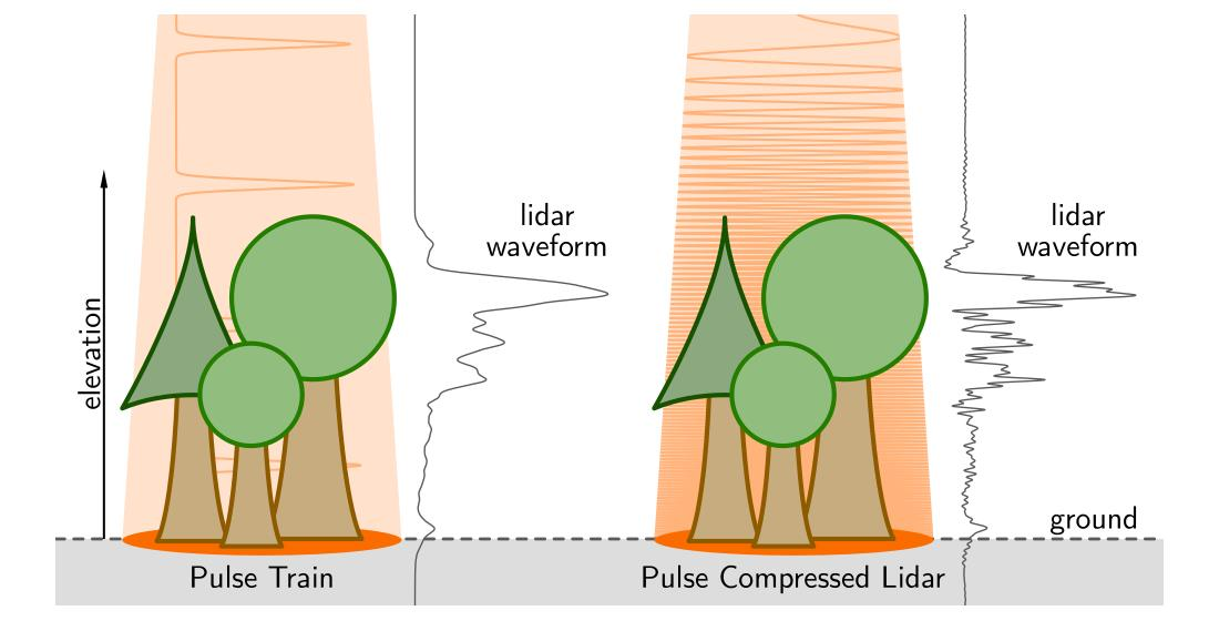
2.3.2. Pulse-Train
2.3.3. Pulse Compressed Lidar (PCL)
Frequency Chirps
Other Pulse Shapes
2.3.4. Phase-Based
2.4. Detectors
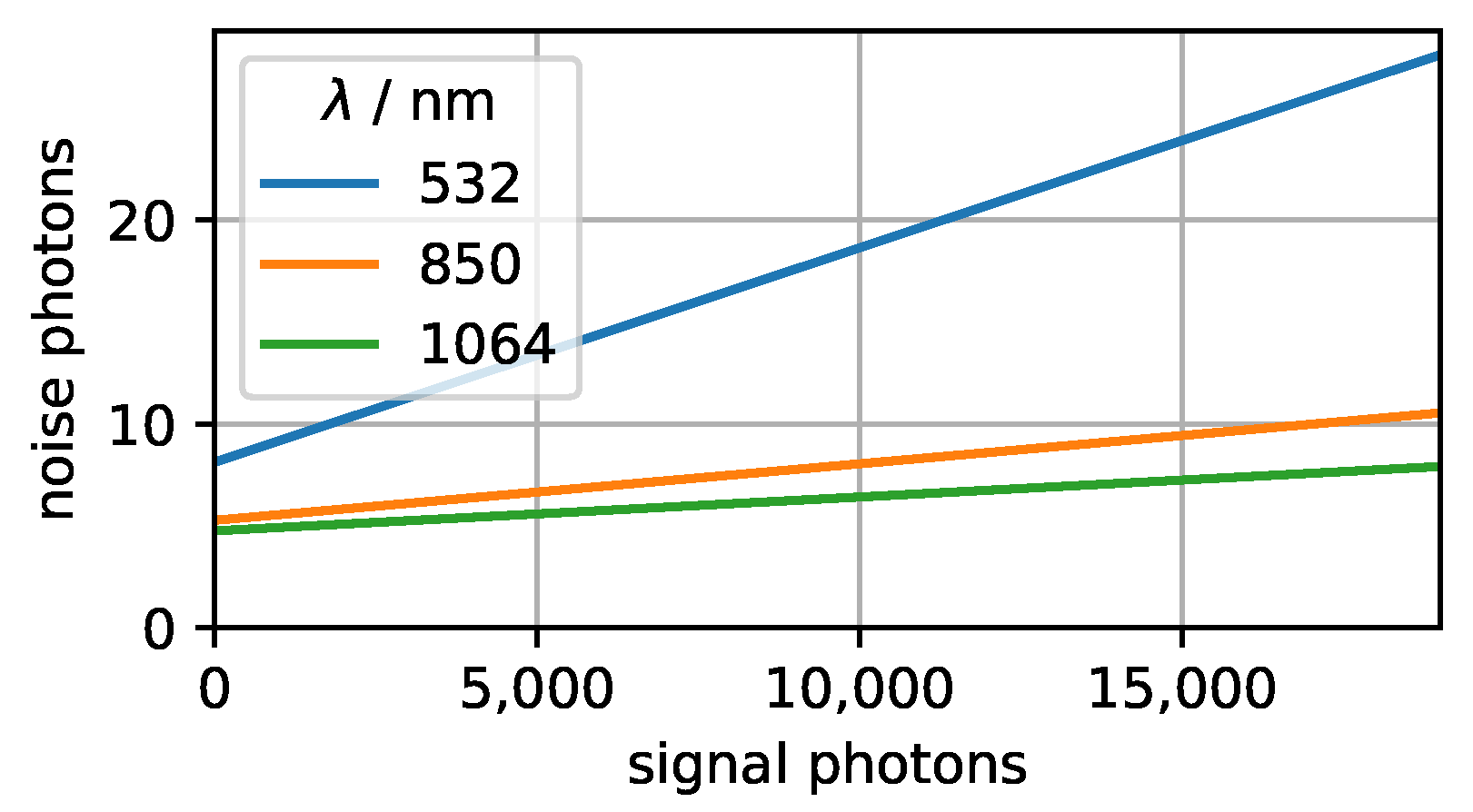
2.5. Estimation of Noise Photons
2.5.1. Lunar Noise
2.5.2. Dark Count
2.5.3. Atmospheric Scattering
2.5.4. Total Noise Rate
- The lunar noise () is proportional to , , A, and Q.
- The dark count () is constant and does not scale with any of the parameters.
- The atmospheric scattering () scales with , A and Q.
2.6. Energy and Power Estimation
3. Methods
3.1. Lidar Simulator
3.1.1. Simulator Validation
3.1.2. Signal Processing
- varScale
- controls the signal detection threshold as a number of standard deviations above background [50];
- minWidth
- controls the minimum number of consecutive bins that must lie above the threshold [50];
- sWidth
- sets the smoothing width in meters;
- hann
- applies a Hann filter with the specified number of bins [51].
3.2. ALS Datasets
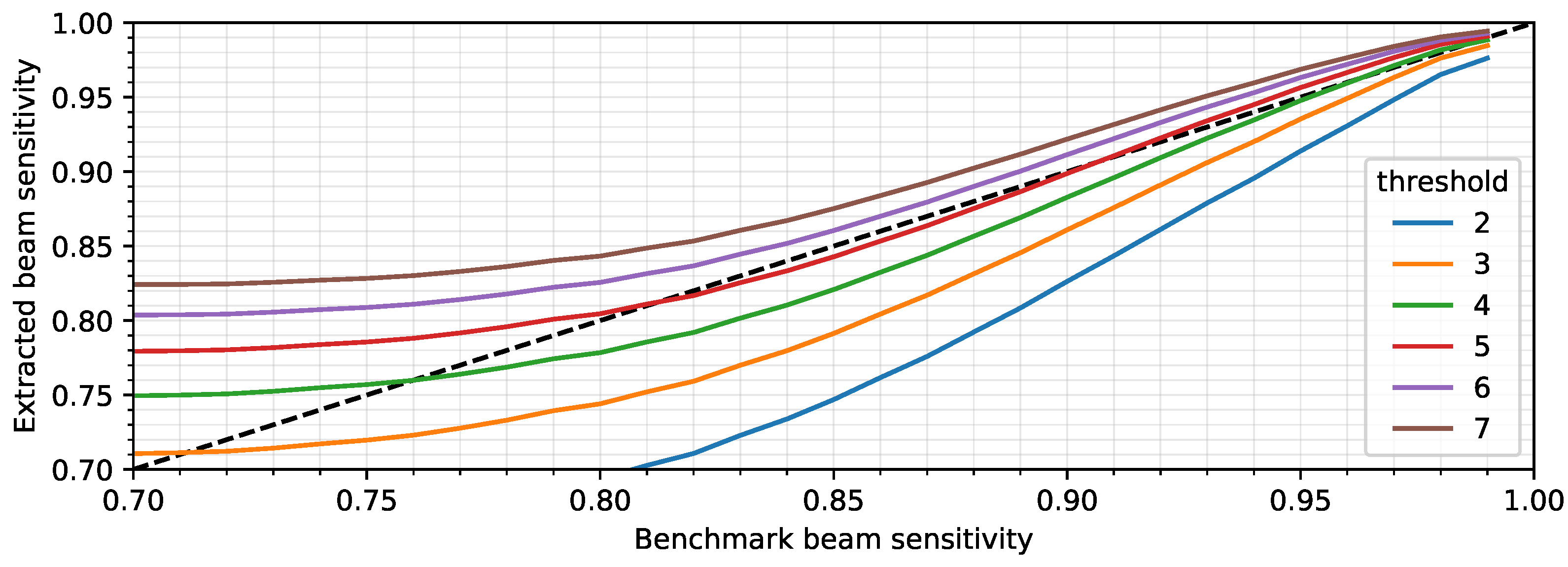
3.3. Beam Sensitivity Calculation
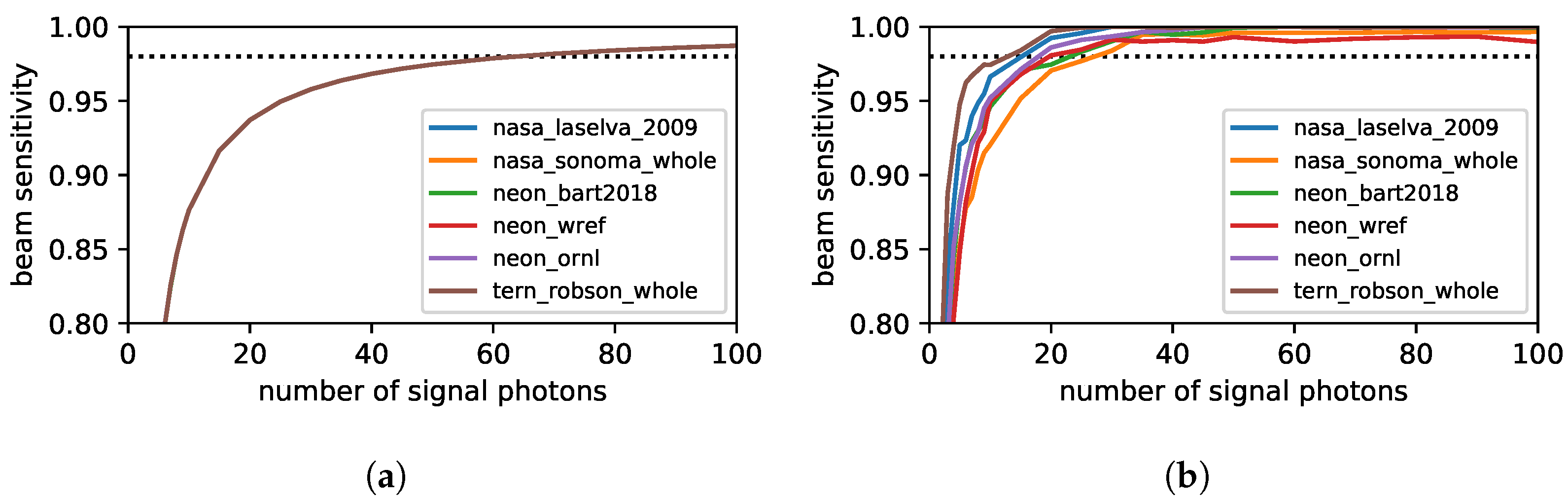
3.3.1. Estimation from Signal-to-Noise Ratio
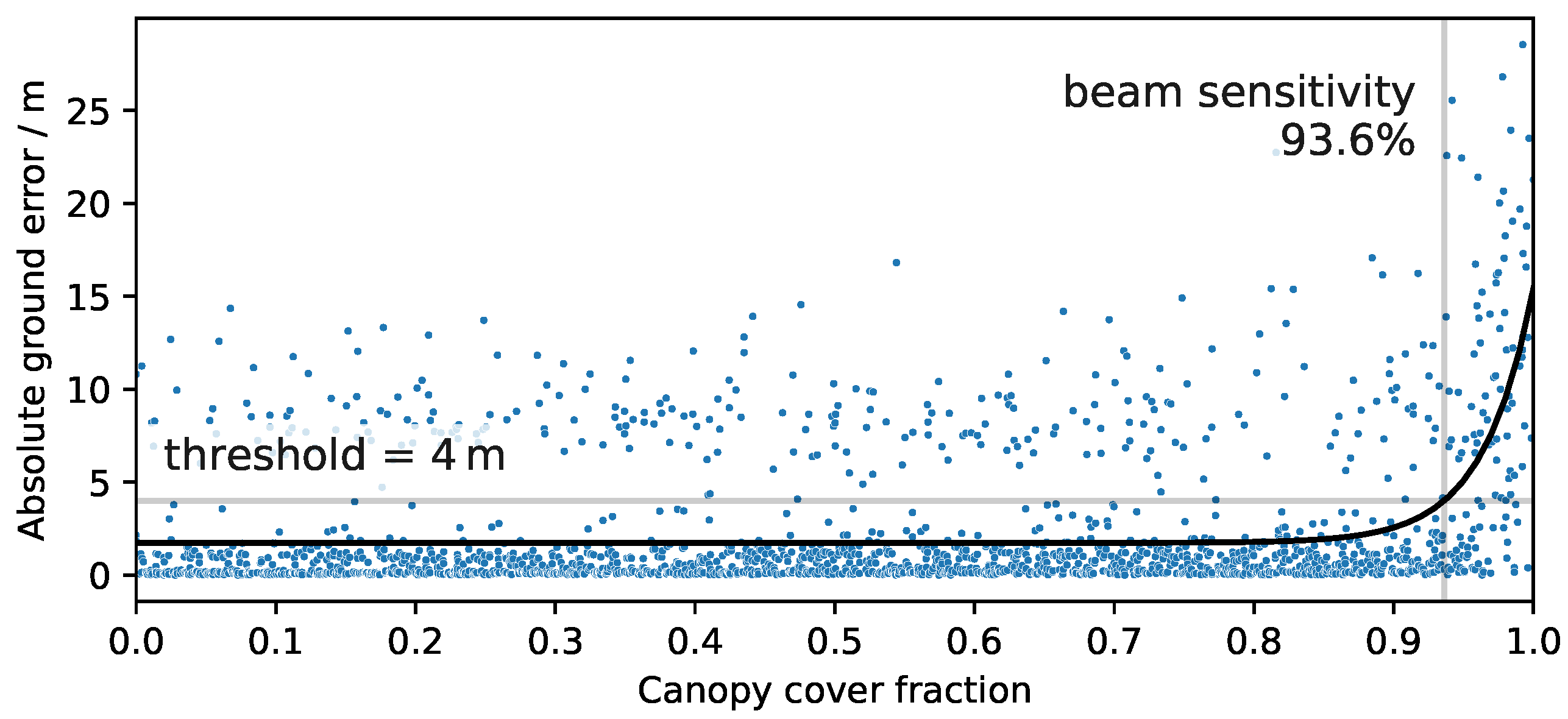
3.3.2. Estimation from Ground Error Distribution
3.4. Experiments
3.4.1. Solid-State Lasers
3.4.2. Diode Lasers
4. Results
4.1. Simulator Validation
4.2. Solid-State Lasers
Photon Counting
4.3. Diode Lasers
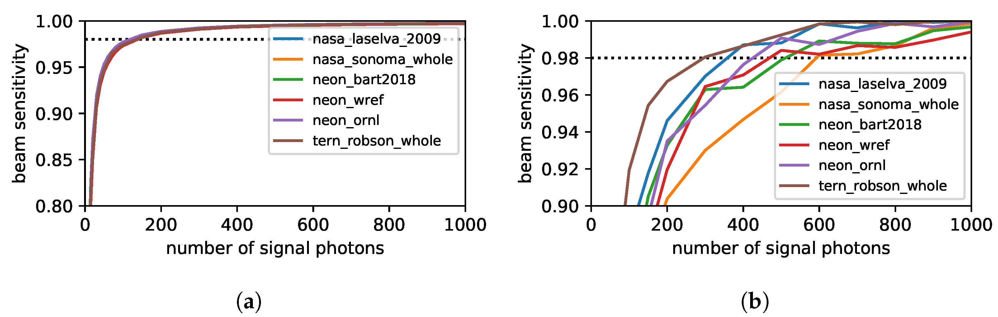
4.3.1. Pulse Train
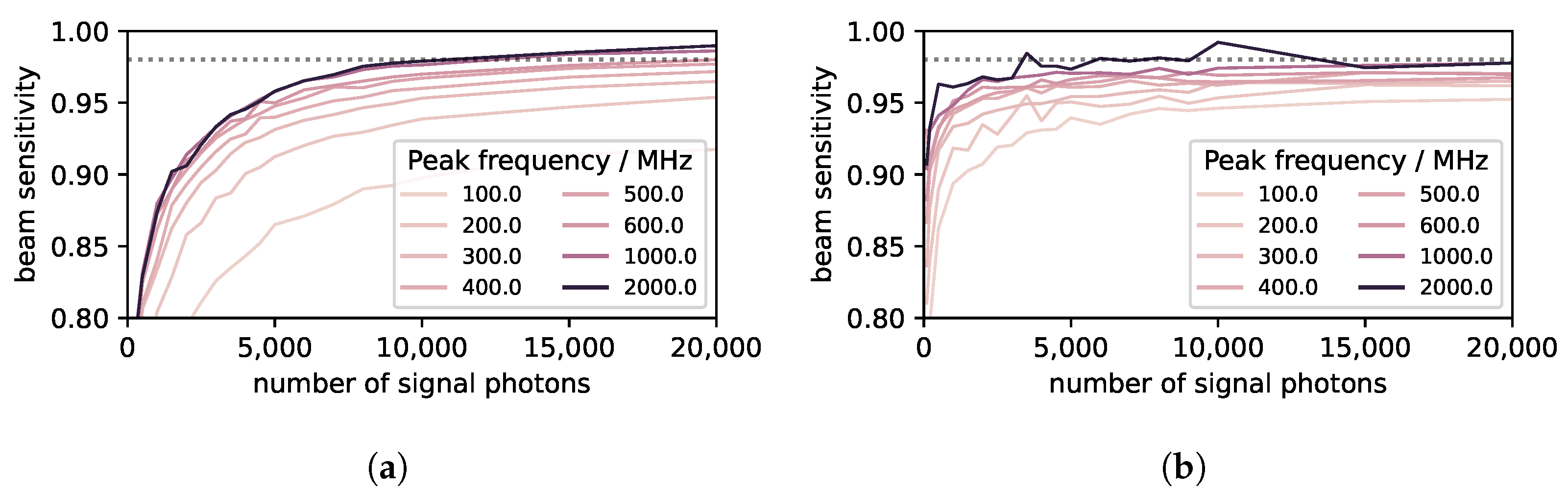
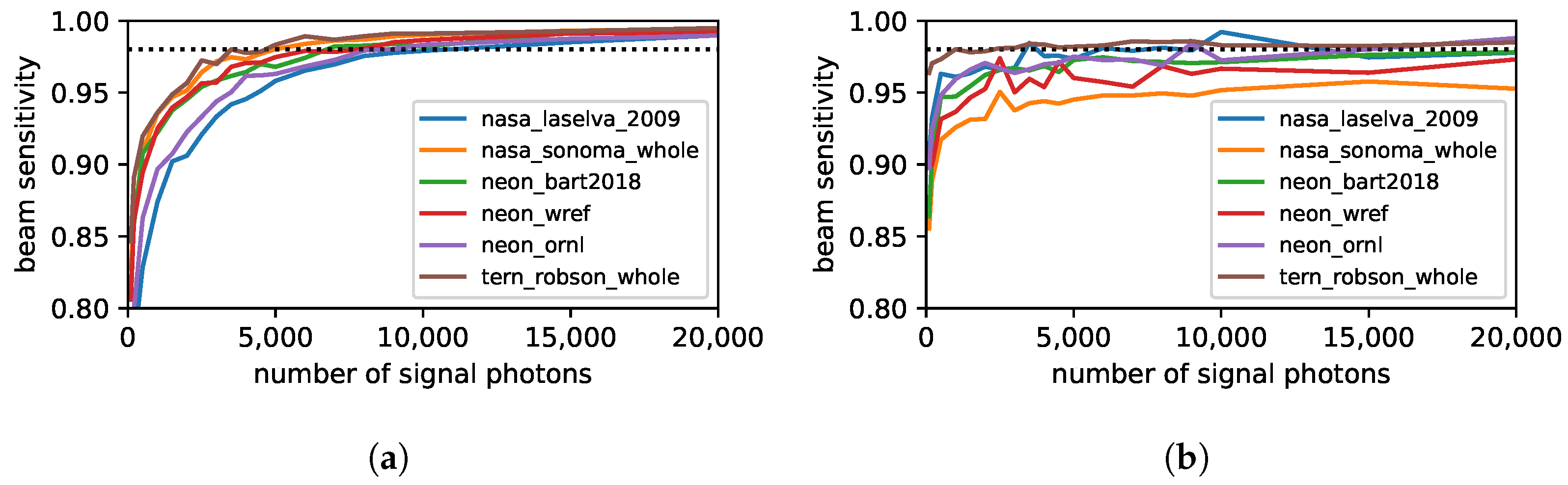
4.3.2. PCL
4.4. Comparison of Values
5. Discussion
6. Conclusions
- (a)
- A solid-state laser with photon-counting detector still requires the lowest detectable energy overall.
- (b)
- Based on energy and power requirements alone, a diode laser with a pulse train configuration can provide a two times wider coverage than a solid-state laser with a swath width of 13,085 m, while at the same time requiring less than 0.1% of the peak power.
- (c)
- Compared to a pulse train, PCL requires significantly larger photon numbers to achieve the same beam sensitivity due to the cross-correlation artifacts introduced by a discrete photon counting return signal. It is therefore probably not the optimum configuration for a diode laser lidar.
- (d)
- The anticipated system cost for global coverage in 5 years can potentially be reduced when using a diode laser compared to a solid-state laser, as the same coverage may be achieved with a smaller satellite.
Author Contributions
Funding
Data Availability Statement
Acknowledgments
Conflicts of Interest
Abbreviations
| ADC | analog-to-digital converter |
| ALS | Airborne Laser Scanning |
| CW | Continuous Wave |
| FWHM | full-width half maximum |
| MLS | maximum length sequence |
| PCL | Pulse Compressed Lidar |
| PDE | photon detection efficiency |
| SiPM | silicon photomultiplier |
| SNR | signal-to-noise ratio |
| SPAD | single photon avalanche diode |
| TEC | thermo-electric cooling |
| TRL | technology readiness level |
Appendix A. Calculating Average and Peak Power
Appendix B. Beam Sensitivity Benchmark
References
- Sun, G.; Ranson, K.; Kimes, D.; Blair, J.; Kovacs, K. Forest vertical structure from GLAS: An evaluation using LVIS and SRTM data. Remote Sens. Environ. 2008, 112, 107–117. [Google Scholar] [CrossRef]
- Dubayah, R.; Blair, J.B.; Goetz, S.; Fatoyinbo, L.; Hansen, M.; Healey, S.; Hofton, M.; Hurtt, G.; Kellner, J.; Luthcke, S.; et al. The Global Ecosystem Dynamics Investigation: High-resolution laser ranging of the Earth’s forests and topography. Sci. Remote Sens. 2020, 1, 100002. [Google Scholar] [CrossRef]
- Markus, T.; Neumann, T.; Martino, A.; Abdalati, W.; Brunt, K.; Csatho, B.; Farrell, S.; Fricker, H.; Gardner, A.; Harding, D.; et al. The Ice, Cloud, and land Elevation Satellite-2 (ICESat-2): Science requirements, concept, and implementation. Remote Sens. Environ. 2017, 190, 260–273. [Google Scholar] [CrossRef]
- Duncanson, L.; Neuenschwander, A.; Hancock, S.; Thomas, N.; Fatoyinbo, T.; Simard, M.; Silva, C.A.; Armston, J.; Luthcke, S.B.; Hofton, M.; et al. Biomass estimation from simulated GEDI, ICESat-2 and NISAR across environmental gradients in Sonoma County, California. Remote Sens. Environ. 2020, 242, 111779. [Google Scholar] [CrossRef]
- Schneider, F.D.; Ferraz, A.; Hancock, S.; Duncanson, L.I.; Dubayah, R.O.; Pavlick, R.P.; Schimel, D.S. Towards mapping the diversity of canopy structure from space with GEDI. Environ. Res. Lett. 2020, 15, 115006. [Google Scholar] [CrossRef]
- Patterson, P.L.; Healey, S.P.; Ståhl, G.; Saarela, S.; Holm, S.; Andersen, H.E.; Dubayah, R.O.; Duncanson, L.; Hancock, S.; Armston, J.; et al. Statistical properties of hybrid estimators proposed for GEDI—NASA’s global ecosystem dynamics investigation. Environ. Res. Lett. 2019, 14, 065007. [Google Scholar] [CrossRef]
- Friedlingstein, P.; O’sullivan, M.; Jones, M.W.; Andrew, R.M.; Hauck, J.; Olsen, A.; Peters, G.P.; Peters, W.; Pongratz, J.; Sitch, S.; et al. Global carbon budget 2020. Earth Syst. Sci. Data 2020, 12, 3269–3340. [Google Scholar] [CrossRef]
- Healey, S.P.; Yang, Z.; Gorelick, N.; Ilyushchenko, S. Highly local model calibration with a new GEDI LiDAR asset on Google Earth Engine reduces landsat forest height signal saturation. Remote Sens. 2020, 12, 2840. [Google Scholar] [CrossRef]
- Mitchard, E.T.; Saatchi, S.S.; White, L.; Abernethy, K.; Jeffery, K.J.; Lewis, S.L.; Collins, M.; Lefsky, M.A.; Leal, M.E.; Woodhouse, I.H.; et al. Mapping tropical forest biomass with radar and spaceborne LiDAR in Lopé National Park, Gabon: Overcoming problems of high biomass and persistent cloud. Biogeosciences 2012, 9, 179–191. [Google Scholar] [CrossRef] [Green Version]
- Qi, W.; Lee, S.K.; Hancock, S.; Luthcke, S.; Tang, H.; Armston, J.; Dubayah, R. Improved forest height estimation by fusion of simulated GEDI Lidar data and TanDEM-X InSAR data. Remote Sens. Environ. 2019, 221, 621–634. [Google Scholar] [CrossRef] [Green Version]
- Silva, C.A.; Duncanson, L.; Hancock, S.; Neuenschwander, A.; Thomas, N.; Hofton, M.; Fatoyinbo, L.; Simard, M.; Marshak, C.Z.; Armston, J.; et al. Fusing simulated GEDI, ICESat-2 and NISAR data for regional aboveground biomass mapping. Remote Sens. Environ. 2021, 253, 112234. [Google Scholar] [CrossRef]
- Saatchi, S.S.; Harris, N.L.; Brown, S.; Lefsky, M.; Mitchard, E.T.; Salas, W.; Zutta, B.R.; Buermann, W.; Lewis, S.L.; Hagen, S.; et al. Benchmark map of forest carbon stocks in tropical regions across three continents. Proc. Natl. Acad. Sci. USA 2011, 108, 9899–9904. [Google Scholar] [CrossRef] [Green Version]
- Baccini, A.; Goetz, S.; Walker, W.; Laporte, N.; Sun, M.; Sulla-Menashe, D.; Hackler, J.; Beck, P.; Dubayah, R.; Friedl, M.; et al. Estimated carbon dioxide emissions from tropical deforestation improved by carbon-density maps. Nat. Clim. Chang. 2012, 2, 182–185. [Google Scholar] [CrossRef]
- Avitabile, V.; Herold, M.; Heuvelink, G.B.; Lewis, S.L.; Phillips, O.L.; Asner, G.P.; Armston, J.; Ashton, P.S.; Banin, L.; Bayol, N.; et al. An integrated pan-tropical biomass map using multiple reference datasets. Glob. Chang. Biol. 2016, 22, 1406–1420. [Google Scholar] [CrossRef] [PubMed] [Green Version]
- Hill, T.C.; Williams, M.; Bloom, A.A.; Mitchard, E.T.; Ryan, C.M. Are inventory based and remotely sensed above-ground biomass estimates consistent? PLoS ONE 2013, 8, e74170. [Google Scholar] [CrossRef] [PubMed] [Green Version]
- Ploton, P.; Mortier, F.; Réjou-Méchain, M.; Barbier, N.; Picard, N.; Rossi, V.; Dormann, C.; Cornu, G.; Viennois, G.; Bayol, N.; et al. Spatial validation reveals poor predictive performance of large-scale ecological mapping models. Nat. Commun. 2020, 11, 1–11. [Google Scholar] [CrossRef]
- Hancock, S.; Mcgrath, C.; Lowe, C.; Woodhouse, I. Requirements for a spaceborne lidar with wall-to-wall coverage: A Global Lidar System. R. Soc. Open Sci. 2021, 8, 1–17. [Google Scholar] [CrossRef]
- Harding, D.J.; Carabajal, C.C. ICESat waveform measurements of within-footprint topographic relief and vegetation vertical structure. Geophys. Res. Lett. 2005, 32. [Google Scholar] [CrossRef] [Green Version]
- Hancock, S.; Lewis, P.; Foster, M.; Disney, M.; Muller, J.P. Measuring forests with dual wavelength lidar: A simulation study over topography. Agric. For. Meteorol. 2012, 161, 123–133. [Google Scholar] [CrossRef] [Green Version]
- Hancock, S.; Armston, J.; Hofton, M.; Sun, X.; Tang, H.; Duncanson, L.I.; Kellner, J.R.; Dubayah, R. The GEDI Simulator: A Large-Footprint Waveform Lidar Simulator for Calibration and Validation of Spaceborne Missions. Earth Space Sci. 2019, 6, 294–310. [Google Scholar] [CrossRef]
- Hofton, M.A.; Minster, J.B.; Blair, J.B. Decomposition of laser altimeter waveforms. IEEE Trans. Geosci. Remote Sens. 2000, 38, 1989–1996. [Google Scholar] [CrossRef]
- Hancock, S.; Lewis, P.; Disney, M.; Foster, M.; Muller, J.P. Assessing the Accuracy of Forest Height Estimation with Long Pulse Waveform Lidar Through Monte-Carlo Ray Tracing. In Proceedings of the Silvilaser, Edinburgh, UK, 17–19 September 2008; pp. 199–206. [Google Scholar]
- Winker, D.M.; Couch, R.H.; McCormick, M. An overview of LITE: NASA’s lidar in-space technology experiment. Proc. IEEE 1996, 84, 164–180. [Google Scholar] [CrossRef]
- Schutz, B.E.; Zwally, H.J.; Shuman, C.A.; Hancock, D.; DiMarzio, J.P. Overview of the ICESat mission. Geophys. Res. Lett. 2005, 32. [Google Scholar] [CrossRef] [Green Version]
- Winker, D.M.; Vaughan, M.A.; Omar, A.; Hu, Y.; Powell, K.A.; Liu, Z.; Hunt, W.H.; Young, S.A. Overview of the CALIPSO mission and CALIOP data processing algorithms. J. Atmos. Ocean. Technol. 2009, 26, 2310–2323. [Google Scholar] [CrossRef]
- Stoffelen, A.; Marseille, G.; Bouttier, F.; Vasiljevic, D.; De Haan, S.; Cardinali, C. ADM-Aeolus Doppler wind lidar observing system simulation experiment. Q. J. R. Meteorol. Soc. A J. Atmos. Sci. Appl. Meteorol. Phys. Oceanogr. 2006, 132, 1927–1947. [Google Scholar] [CrossRef]
- McGill, M.J.; Yorks, J.E.; Scott, V.S.; Kupchock, A.W.; Selmer, P.A. The Cloud-Aerosol Transport System (CATS): A technology demonstration on the International Space Station. In Lidar Remote Sensing for Environmental Monitoring XV; International Society for Optics and Photonics: Bellingham, WA, USA, 2015; Volume 9612, p. 96120A. [Google Scholar]
- Stysley, P.R.; Coyle, D.B.; Kay, R.B.; Frederickson, R.; Poulios, D.; Cory, K.; Clarke, G. Long term performance of the High Output Maximum Efficiency Resonator (HOMER) laser for NASA’s Global Ecosystem Dynamics Investigation (GEDI) lidar. Opt. Laser Technol. 2015, 68, 67–72. [Google Scholar] [CrossRef]
- Konoplev, O.A.; Chiragh, F.L.; Vasilyev, A.A.; Edwards, R.; Stephen, M.A.; Troupaki, E.; Yu, A.W.; Krainak, M.A.; Sawruk, N.; Hovis, F.; et al. Three-year aging of prototype flight laser at 10 kHz and 1 ns pulses with external frequency doubler for ICESat-2 mission. In Proceedings of the Laser Technology for Defense and Security XII, Baltimore, MD, USA, 19–20 April 2016; Volume 9834, p. 98340A. [Google Scholar] [CrossRef] [Green Version]
- Abshire, J.B.; Sun, X.; Mazarico, E.; Head III, J.W.; Yu, A.W.; Beck, J.D. A 3-D Surface Imaging Lidar for Mapping Mars and Other Bodies from Orbit. In Proceedings of the 51st Lunar and Planetary Science Conference, The Woodlands, TX, USA, 16–20 March 2020; p. 1966. [Google Scholar]
- Kelemen, M.; Neukum, J. Semiconductor Tapered Amplifiers as a Tool for Quantum Technologies and LiDAR. Coherent Webinar. 2021. Available online: https://www.coherent.com/events/webinars (accessed on 4 April 2022).
- European Thermodynamics Ltd. ET-071-10-13 Peltier Cooler Module. 2020. Available online: https://docs.rs-online.com/c588/0900766b8144a9b9.pdf (accessed on 4 April 2022).
- Ziegler, M.; Hempel, M.; Larsen, H.E.; Tomm, J.W.; Andersen, P.E.; Clausen, S.; Elliott, S.N.; Elsaesser, T. Physical limits of semiconductor laser operation: A time-resolved analysis of catastrophic optical damage. Appl. Phys. Lett. 2010, 97, 10–13. [Google Scholar] [CrossRef] [Green Version]
- Neuenschwander, A.; Pitts, K. The ATL08 land and vegetation product for the ICESat-2 Mission. Remote Sens. Environ. 2019, 221, 247–259. [Google Scholar] [CrossRef]
- Yang, J.; Zhao, B.; Liu, B. Coherent Pulse-Compression Lidar Based on 90-Degree Optical Hybrid. Sensors 2019, 19, 4570. [Google Scholar] [CrossRef] [Green Version]
- Sarwate, D.V.; Pursley, M.B. Crosscorrelation properties of pseudorandom and related sequences. Proc. IEEE 1980, 68, 593–619. [Google Scholar] [CrossRef]
- Chu, D. Polyphase codes with good periodic correlation properties (corresp.). IEEE Trans. Inf. Theory 1972, 18, 531–532. [Google Scholar] [CrossRef]
- Popovic, B. Generalized chirp-like polyphase sequences with optimum correlation properties. IEEE Trans. Inf. Theory 1992, 38, 1406–1409. [Google Scholar] [CrossRef]
- Newnham, G.; Armston, J.; Muir, J.; Goodwin, N.; Tindall, D.; Culvenor, D.; Püschel, P.; Nyström, M.; Johansen, K. Evaluation of Terrestrial Laser Scanners for Measuring Vegetation Structure; CSIRO: Canberra, Australia, 2012.
- Barton-Grimley, R.A.; Thayer, J.P.; Hayman, M. Nonlinear target count rate estimation in single-photon lidar due to first photon bias. Opt. Lett. 2019, 44, 1249–1252. [Google Scholar] [CrossRef] [PubMed]
- Yang, G.; Martino, A.J.; Lu, W.; Cavanaugh, J.; Bock, M.; Krainak, M.A. IceSat-2 ATLAS photon-counting receiver: Initial on-orbit performance. In Proceedings of the Advanced Photon Counting Techniques XIII, Baltimore, MD, USA, 17–18 April 2019; International Society for Optics and Photonics: Bellingham, WA, USA, 2019; Volume 10978, p. 109780B. [Google Scholar]
- Morimoto, K.; Charbon, E. High fill-factor miniaturized SPAD arrays with a guard-ring-sharing technique. Opt. Express 2020, 28, 13068–13080. [Google Scholar] [CrossRef] [PubMed]
- Ito, K.; Otake, Y.; Kitano, Y.; Matsumoto, A.; Yamamoto, J.; Ogasahara, T.; Hiyama, H.; Naito, R.; Takeuchi, K.; Tada, T.; et al. A Back Illuminated 10 μm SPAD Pixel Array Comprising Full Trench Isolation and Cu-Cu Bonding with over 14% PDE at 940 nm. In Proceedings of the 2020 IEEE International Electron Devices Meeting (IEDM), San Francisco, CA, USA, 12–18 December 2020; IEEE: Piscataway, NJ, USA, 2020; pp. 16.6.1–16.6.4. [Google Scholar]
- Kumagai, O.; Ohmachi, J.; Matsumura, M.; Yagi, S.; Tayu, K.; Amagawa, K.; Matsukawa, T.; Ozawa, O.; Hirono, D.; Shinozuka, Y.; et al. A 189 × 600 Back-Illuminated Stacked SPAD Direct Time-of-Flight Depth Sensor for Automotive LiDAR Systems. In Proceedings of the 2021 IEEE International Solid-State Circuits Conference (ISSCC), San Francisco, CA, USA, 13–22 February 2021; IEEE: Piscataway, NJ, USA, 2021; Volume 64, pp. 110–112. [Google Scholar]
- Excelitas. SPCM-NIR: NIR-Optimized Single Photon Counting Module. 2020. Available online: https://www.excelitas.com/product/spcm-nir (accessed on 4 April 2022).
- Giudice, A.; Ghioni, M.; Biasi, R.; Zappa, F.; Cova, S.; Maccagnani, P.; Gulinatti, A. High-rate photon counting and picosecond timing with silicon-SPAD based compact detector modules. J. Mod. Opt. 2007, 54, 225–237. [Google Scholar] [CrossRef]
- Henderson, R.K.; Johnston, N.; Della Rocca, F.M.; Chen, H.; Li, D.D.U.; Hungerford, G.; Hirsch, R.; McLoskey, D.; Yip, P.; Birch, D.J. A 192 × 128 Time Correlated SPAD Image Sensor in 40-nm CMOS Technology. IEEE J. Solid-State Circuits 2019, 54, 1907–1916. [Google Scholar] [CrossRef] [Green Version]
- Blair, J.B.; Hofton, M.A. Modeling laser altimeter return waveforms over complex vegetation using high-resolution elevation data. Geophys. Res. Lett. 1999, 26, 2509–2512. [Google Scholar] [CrossRef]
- Duncanson, L.; Kellner, J.R.; Armston, J.; Dubayah, R.; Minor, D.M.; Hancock, S.; Healey, S.P.; Patterson, P.L.; Saarela, S.; Marselis, S.; et al. Aboveground biomass density models for NASA’s Global Ecosystem Dynamics Investigation (GEDI) lidar mission. Remote Sens. Environ. 2022, 270, 112845. [Google Scholar] [CrossRef]
- Hancock, S.; Anderson, K.; Disney, M.; Gaston, K.J. Measurement of fine-spatial-resolution 3D vegetation structure with airborne waveform lidar: Calibration and validation with voxelised terrestrial lidar. Remote Sens. Environ. 2017, 188, 37–50. [Google Scholar] [CrossRef] [Green Version]
- Kahlig, P. Some aspects of Julius von Hann’s contribution to modern climatology. Geophys.-Monogr.-Am. Geophys. Union 1993, 75, 1–7. [Google Scholar]
- OpenTopography. UMD-NASA Carbon Mapping/Sonoma County Vegetation Mapping and LiDAR Program; OpenTopography: La Jolla, CA, USA, 2014. [Google Scholar] [CrossRef]
- OpenTopography. TEAM Lidar Data Over La Selva, Costa Rica 2009; OpenTopography: La Jolla, CA, USA, 2019. [Google Scholar] [CrossRef]
- National Ecological Observatory Network (NEON). Elevation—LiDAR (DP3.30024.001); National Ecological Observatory Network (NEON): Boulder, CO, USA, 2021. [Google Scholar] [CrossRef]
- TERN AusCover. FNQR Robson Creek—Airborne LiDAR Survey, 2012. Made Available by the AusCover Facility of the Terrestrial Ecosystem Research Network (TERN). Available online: http://www.auscover.org.au (accessed on 4 April 2022).
- Neumann, T.A.; Brenner, A.; Hancock, D.; Robbins, J.; Saba, J.; Harbeck, K.; Gibbons, A.; Lee, J.; Luthcke, S.B.; Rebold, T.; et al. ATLAS/ICESat-2 L2A Global Geolocated Photon Data, Version 4; NSIDC NASA DAAC: National Snow and Ice Data Center: Boulder, CO, USA, 2021. [Google Scholar] [CrossRef]
- Applied Research Laboratories. PhoREAL, Version 3.24; University of Texas: Austin, TX, USA, 2020. [Google Scholar]


| Instrument | Pulse Rate (Hz) | (mJ) | Number Tracks | (W) | (kW) | (nm) | Detector type a | Db (cm) | Hc (km) | In Orbit |
|---|---|---|---|---|---|---|---|---|---|---|
| ICESat | 40 | 100 | 1 | 4.0 | 8300 | 1064, 532 | FW | 80 | 600 | 2003–2009 |
| CALIPSO | 20 | 110 | 1 | 2.2 | 2750 | 1064, 532 | FW | 100 | 705 | 2006– |
| CATS | 10,000/5000 | 1–2 | 3 | 15.0 | 1064, 532, 355 | PC | 60 | 400 | 2015–2017 | |
| Aeolus | 51 | 110 | 1 | 5.6 | 2750 | 355 | FW | 150 | 320 | 2018– |
| ICESat-2 | 10,000 | 1.2 | 6 | 12.0 | 400 | 532 | PC | 80 | 481 | 2018– |
| GEDI | 242 | 10 | 8 | 7.3 | 320 | 1064 | FW | 80 | 420 | 2018– |
| Laser Source: | Solid-State | Diode | |
|---|---|---|---|
| Lidar Modality: | Single Pulse | Pulse Train | PCL |
| Q | 0.31 | 0.58 | 0.58 |
| 30 pm | 1 nm | 1 nm | |
| 1 | 4000 | 4000 | |
| Integration time | 1 | 4 ms | 4 ms |
| Noise rate/μs−1 | 8.1 | 1.32 | 1.32 |
| Noise rate/mJ−1 | 0.067 | 0.125 | 0.125 |
| Site | Biome | Canopy Cover (%) | Ground Elevation (m) | Ground Slope (Degree) | Canopy Height (m) | Reference |
|---|---|---|---|---|---|---|
| Sonoma | Mediterranean Forests, Woodlands and Scrub | 65 ± 30 | 208 ± 80 | 18 ± 11 | 25 ± 14 | [52] |
| La Selva | Tropical and Subtropical Moist Broadleaf Forests | 68 ± 36 | 77 ± 35 | 10.0 ± 9.1 | 22 ± 12 | [53] |
| Bartlett | Temperate Broadleaf and Mixed Forests | 84 ± 20 | 510 ± 170 | 16.1 ± 9.4 | 19.3 ± 5.2 | [54] |
| Wind River | Temperate Conifer Forests | 75 ± 18 | 680 ± 240 | 18 ± 12 | 32 ± 12 | [54] |
| Robson Creek | Tropical and Subtropical Grasslands, Savannas and Shrublands | 97.7 ± 3.5 | 860 ± 140 | 22 ± 10 | 32.7 ± 5.6 | [55] |
| Oak Ridge | Temperate Broadleaf and Mixed Forests | 63 ± 39 | 272 ± 31 | 9.3 ± 7.7 | 19 ± 11 | [54] |
| Source | Solid-State | Diode | |||
|---|---|---|---|---|---|
| Modality | Single Pulse | Pulse Train | PCL | ||
| Detector | Full Waveform | Photon Counting | Photon Counting | Photon Counting | |
| scenario conditions { | Q | 0.58 | 0.31 | 0.58 | |
| 0.11 | 0.25 | ||||
| 1 | 4000 | ||||
| 0.7 nm | 30 pm | 1 nm | |||
| T | ≈1 | ≈1 | 4 ms | ||
| at 98% sensitivity { | 1500 a | 60 | 115 | 11,400 | |
| n/a | 0.02 | 5.3 | 8.4 | ||
| 0.28 | 0.014 | 0.027 | 2.66 | ||
| 2.6 mJ b | 0.25 mJ | 0.25 mJ | 25.2 mJ | ||
| 79.7 kW b | 7.5 kW | 1.9 | 14.9 | ||
| 0.66 b | 0.06 | 0.06 | 6.3 | ||
| swath | 553 m | 5898 m | 13,085 m | 132 m | |
| 4 | 1 | 1 | 15 | ||
Publisher’s Note: MDPI stays neutral with regard to jurisdictional claims in published maps and institutional affiliations. |
© 2022 by the authors. Licensee MDPI, Basel, Switzerland. This article is an open access article distributed under the terms and conditions of the Creative Commons Attribution (CC BY) license (https://creativecommons.org/licenses/by/4.0/).
Share and Cite
Hansen, J.N.; Hancock, S.; Prade, L.; Bonner, G.M.; Chen, H.; Davenport, I.; Jones, B.E.; Purslow, M. Assessing Novel Lidar Modalities for Maximizing Coverage of a Spaceborne System through the Use of Diode Lasers. Remote Sens. 2022, 14, 2426. https://doi.org/10.3390/rs14102426
Hansen JN, Hancock S, Prade L, Bonner GM, Chen H, Davenport I, Jones BE, Purslow M. Assessing Novel Lidar Modalities for Maximizing Coverage of a Spaceborne System through the Use of Diode Lasers. Remote Sensing. 2022; 14(10):2426. https://doi.org/10.3390/rs14102426
Chicago/Turabian StyleHansen, Johannes N., Steven Hancock, Ludwig Prade, Gerald M. Bonner, Haochang Chen, Ian Davenport, Brynmor E. Jones, and Matthew Purslow. 2022. "Assessing Novel Lidar Modalities for Maximizing Coverage of a Spaceborne System through the Use of Diode Lasers" Remote Sensing 14, no. 10: 2426. https://doi.org/10.3390/rs14102426