Hyperspectral Image Classification Based on Non-Parallel Support Vector Machine

Abstract

Support vector machine (SVM) has a good effect in the supervised classification of hyperspectral images. In view of the shortcomings of the existing parallel structure SVM, this article proposes a non-parallel SVM model. Based on the traditional parallel boundary structure vector machine, this model adds an additional empirical risk minimization term to the original optimization problem by adding the least square term of the sample and obtains two non-parallel hyperplanes, respectively, forming a new non-parallel SVM algorithm to minimize the additional empirical risk of non-parallel SVM (Additional Empirical Risk Minimization Non-parallel Support Vector Machine, AERM-NPSVM). On the basis of AERM-NPSVM, the bias constraint is added to it, and AERM-NPSVM (BC-AERM-NPSVM) is further obtained. The experimental results show that, compared with the traditional parallel SVM model and the classical non-parallel SVM model, Twin Support Vector Machine (TWSVM), the new model, has a better effect in hyperspectral image classification and better generalization performance.

1. Introduction

At present, various technologies of hyperspectral remote sensing have been widely studied [1] and applied to meteorological observation, agricultural production [2], abnormal target detection [3], environmental monitoring [4], military reconnaissance and other fields. Hyperspectral remote sensing data greatly improve the ability of ground object classification and recognition because of their rich spectral information. At present, hyperspectral remote sensing has shown great potential in all aspects of social life, and its application has gone deep into all aspects of life, providing an important technical support for accurate management. The classification of hyperspectral remote sensing images [5,6,7] is one of the important ways for people to obtain information value, and it is a key technology for hyperspectral images to be widely used. Through classification, we can clearly understand the spatial distribution of features and find rules from them. The classification performance directly determines the availability of hyperspectral images. Therefore, hyperspectral image classification has attracted more and more attention and become a research hotspot in the field of remote sensing.

There are many remote sensing image classification algorithms, which can be divided into supervised classification and unsupervised classification according to whether data labels are used in the classification process. The unsupervised classification algorithm means that the samples are classified directly in the classification process without prior information. Its advantage is that the experimental results are less affected by human intervention, and the design parameters of the algorithm are relatively few. Its disadvantage is that when the gap between heterogeneous features is small, the classification effect is poor. The algorithms often used in unsupervised classification are K-means, ISODATA clustering and so on. The supervised classification algorithm first trains the algorithm model under the condition of prior information, and then classifies the test samples when the characteristic parameters of the algorithm model are determined. Its advantage is that the algorithm model can obtain higher classification accuracy through the learning of prior knowledge. The disadvantage is that it is greatly affected by human factors, and the accuracy of classification is affected by the number of training samples to a certain extent. Among the supervised algorithms, the algorithms that are often used in remote sensing data classification are KNN [8], decision tree [9,10] and support vector machine [11,12,13]. Among these algorithms, support vector machine (SVM) has been widely studied and used because of its good performance.

Support vector machine (SVM) is proposed by Vapnik et al., which is suitable for pattern recognition and other fields. The characteristic of SVM is that it can take into account both empirical risk and structural risk, that is, supervised learning can be realized by finding a hyperplane that can not only ensure the accuracy of classification but also maximize the interval between the two types of data [14]. SVM has some good characteristics, such as kernel technique, sparsity and global solution. Because of its solid theoretical foundation and good generalization, it is widely used in remote sensing image classification [15]. The support vector machine classification model presupposes that the positive and negative category boundaries are parallel. However, for the actual remote sensing data, this assumption is difficult to establish, which affects the generalization ability of the model. To solve this problem, Jayadeva et al. proposed Twin Support Vector Machine, (TWSVM) [16,17,18]. The goal of TWSVM is to find a pair of non-parallel hyperplanes (parallel can be regarded as a special state of non-parallel). Each type of data point is close to one of the two non-parallel hyperplanes and is far away from the other, and the category to which it belongs is determined by comparing the distance between the sample and the two hyperplanes. TWSVM is particularly successful, but it still has obvious shortcomings: the TWSVM model only considers the empirical risk but does not consider the structural risk [19], and its generalization performance is affected, so that in many cases, its classification effect is not as good as that of the traditional support vector machine. Kaya, G. T. et al. studied the classification of TWSVM on hyperspectral images [20]. In the linear case, the classification effect of TWSVM is better than that of SVM. In the case of nonlinearity, the classification accuracy of TWSVM has no advantage over SVM. Only using the SVM and TWSVM classification algorithm models for hyperspectral image classification has a limited effect, and some scholars have carried out some research in other directions to further improve the accuracy of hyperspectral image classification. Liu Zhiqiang et al. proposed a remote sensing image classification algorithm based on multi-feature optimization and TWSVM [21]. The features of hyperspectral images are extracted from multiple aspects and combined reasonably, and then TWSVM is used for classification, which improves the accuracy of hyperspectral image classification. Wang, Li-guo et al. proposed a sample reduction algorithm to reduce the size of training samples [22], combined with the least squares twin support vector machine for hyperspectral image classification, speeding up the training speed when the classification accuracy is similar. Wang, Li-guo et al. proposed a semi-supervised classification algorithm for hyperspectral images combining K-means clustering and twin support vector machine [23]. A small amount of labeled supervised information and a large amount of unsupervised information are used to solve the problem of obtaining a large amount of supervised information, thereby reducing the computational complexity of classification and shortening the computational time. There are also some algorithms worth discussing. Inspired by deep neural networks, Onuwa Okwuashi et al. built a deep support vector machine (DSVM) model for hyperspectral data classification by combining deep neural networks and SVM [24]. In the classification performance of hyperspectral images, the classification accuracy of DSVM is better than that of deep neural network and SVM. The purpose of this article is to propose a new non-parallel vector machine algorithm to further improve the classification accuracy of hyperspectral images. A new algorithm model is obtained by modifying the original problem of the support vector machine itself, and this algorithm model is used to improve the effect of hyperspectral image classification. This algorithm does not conflict with the improved algorithm mentioned above, and it is a parallel relationship. For example, the algorithm in this article can be combined with the multi-feature optimization method as in [21] to further optimize the algorithm or to try to replace the hidden layer support vector machine algorithm of the network in [24] with the algorithm in this article. These techniques can be used as future research directions.

In view of the above situation, this article constructs a non-parallel support vector machine model, namely Additional Empirical Risk Minimization Non-parallel Support Vector Machine, AERM-NPSVM, by adding the empirical risk minimization additional term on the basis of the traditional parallel support vector machine. Furthermore, the bias constraint AERM-NPSVM (BC-AERM-NPSVM) is formed by adding the bias constraint to the AERM-NPSVM model. The support vector machine classification model presupposes that the positive and negative category boundaries are parallel. However, hyperspectral datasets do not necessarily meet the above assumptions. These two improved non-parallel support vector machine algorithms based on support vector machines are used to classify hyperspectral images, in the case that the hyperspectral data distribution is not suitable for the SVM parallel plane classification method, to obtain better classification results.

2. Materials and Methods

2.1. Software Description

This project used Python 3.8. Python code which was written on a personal computer using the pycharm software. The processor of the computer is AMD R7 4800 H; random access memory size (RAM) is 16 GB. In this project, functions in the sklearn software toolkit are used to normalize hyperspectral data. The numpy toolkit for matrix computations in algorithmic models was used. The cvxopt toolkit was used to solve convex quadratic programming problems in dual problems.

2.2. Data

The research data are the information of four publicly available hyperspectral scenes. All these are Earth Observation images taken from the air or satellite.

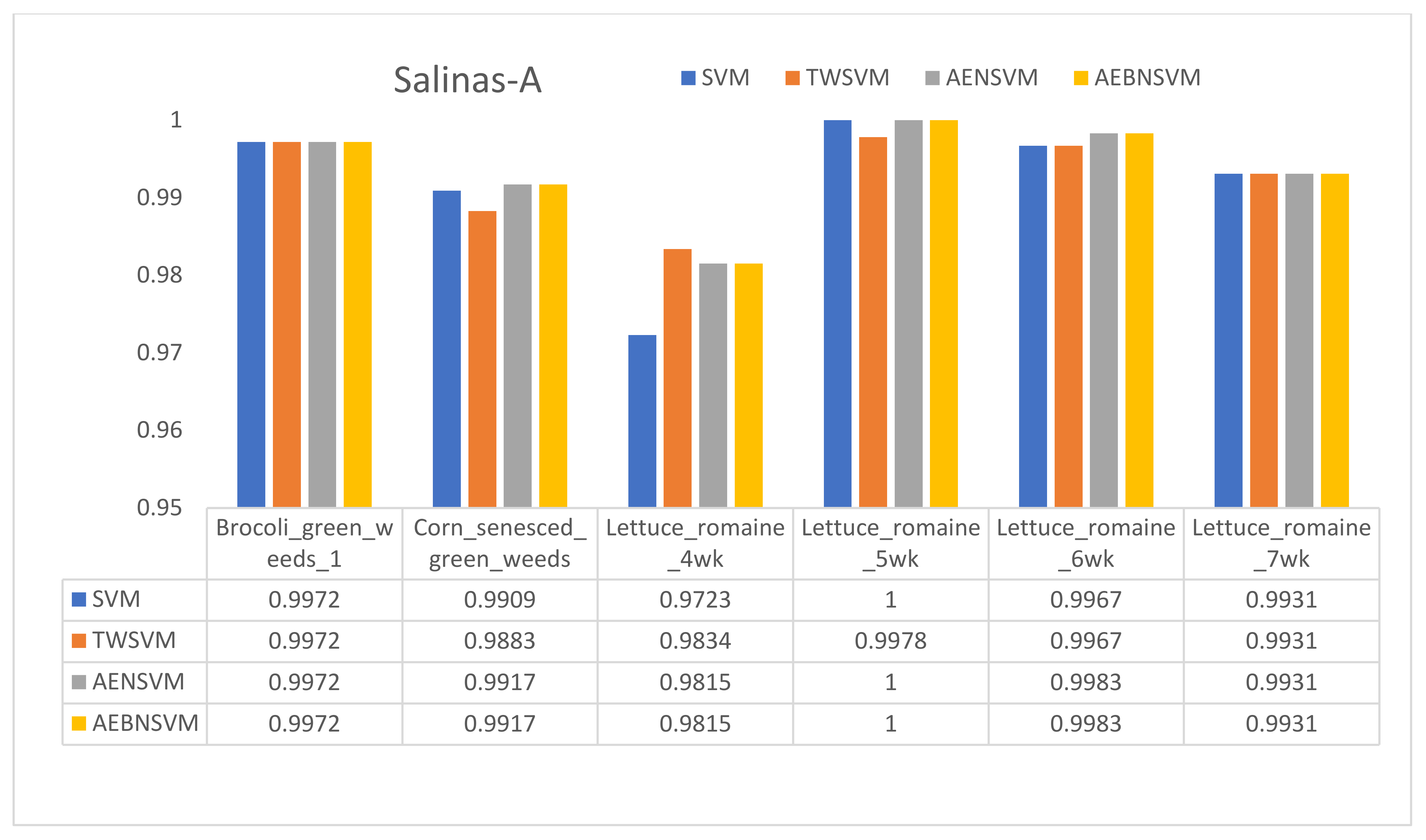
2.2.1. Salinas-A Dataset

The Salinas-A dataset is collected by AVIRIS sensors over the Salinas Valley in California, with a band number of 224, a spatial resolution of 3.7 m and a pixel count of 512 × 217. It consists of 86 × 83 pixels and includes six categories. Figure 1 shows the sample band of the Salinas-A dataset.

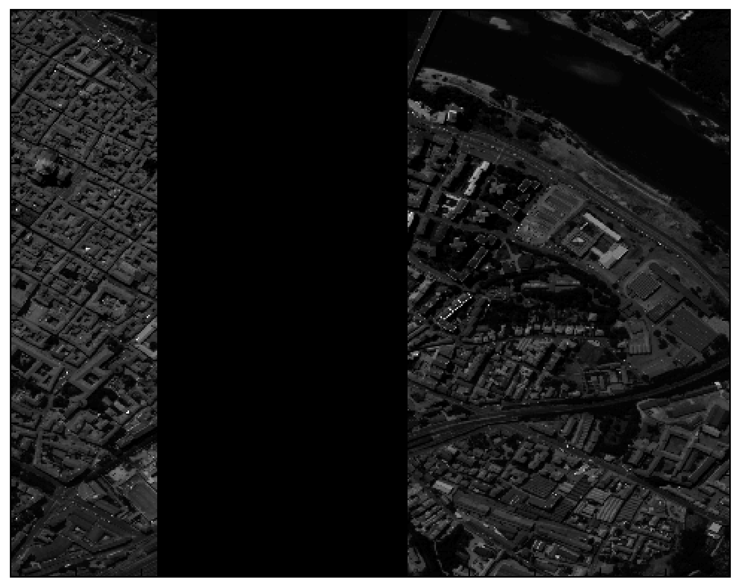
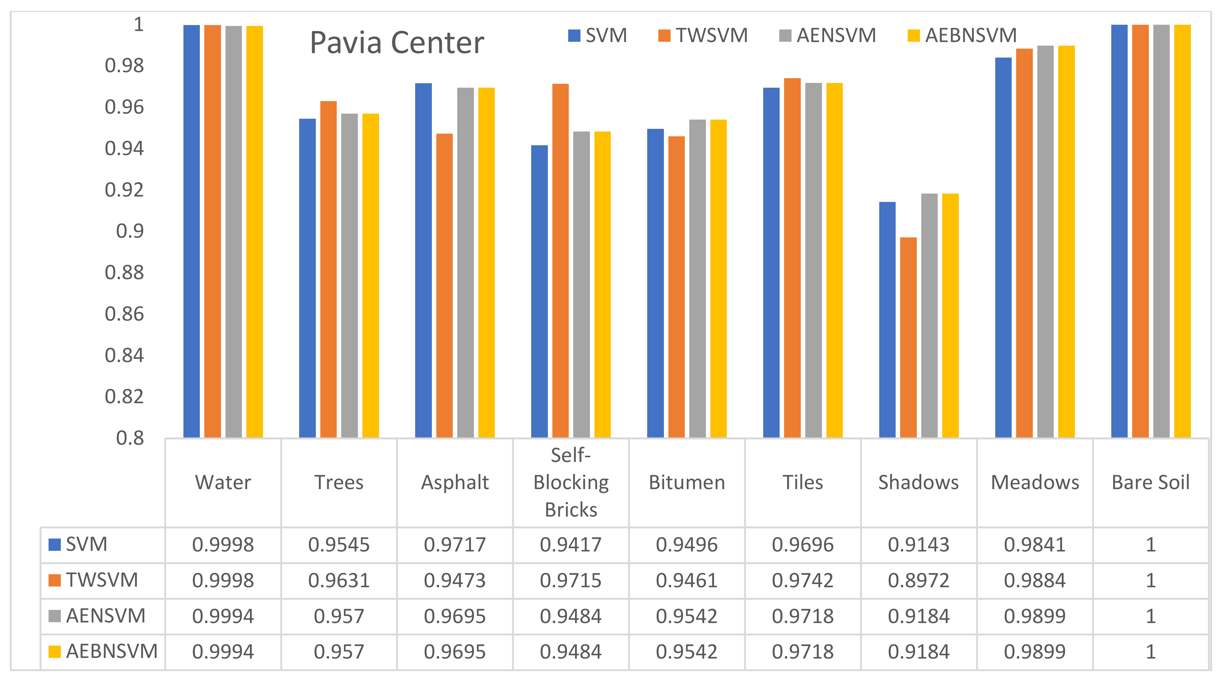
2.2.2. Pavia Center Dataset

The Pavia Center dataset was obtained by the ROSIS sensor in Pavia, northern Italy. The number of spectral bands in the Pavia Center is 102. The Pavia Center is an image with 1096 × 1096 pixels, which contains nine categories. Figure 2 shows the sample band of the Pavia Center dataset.

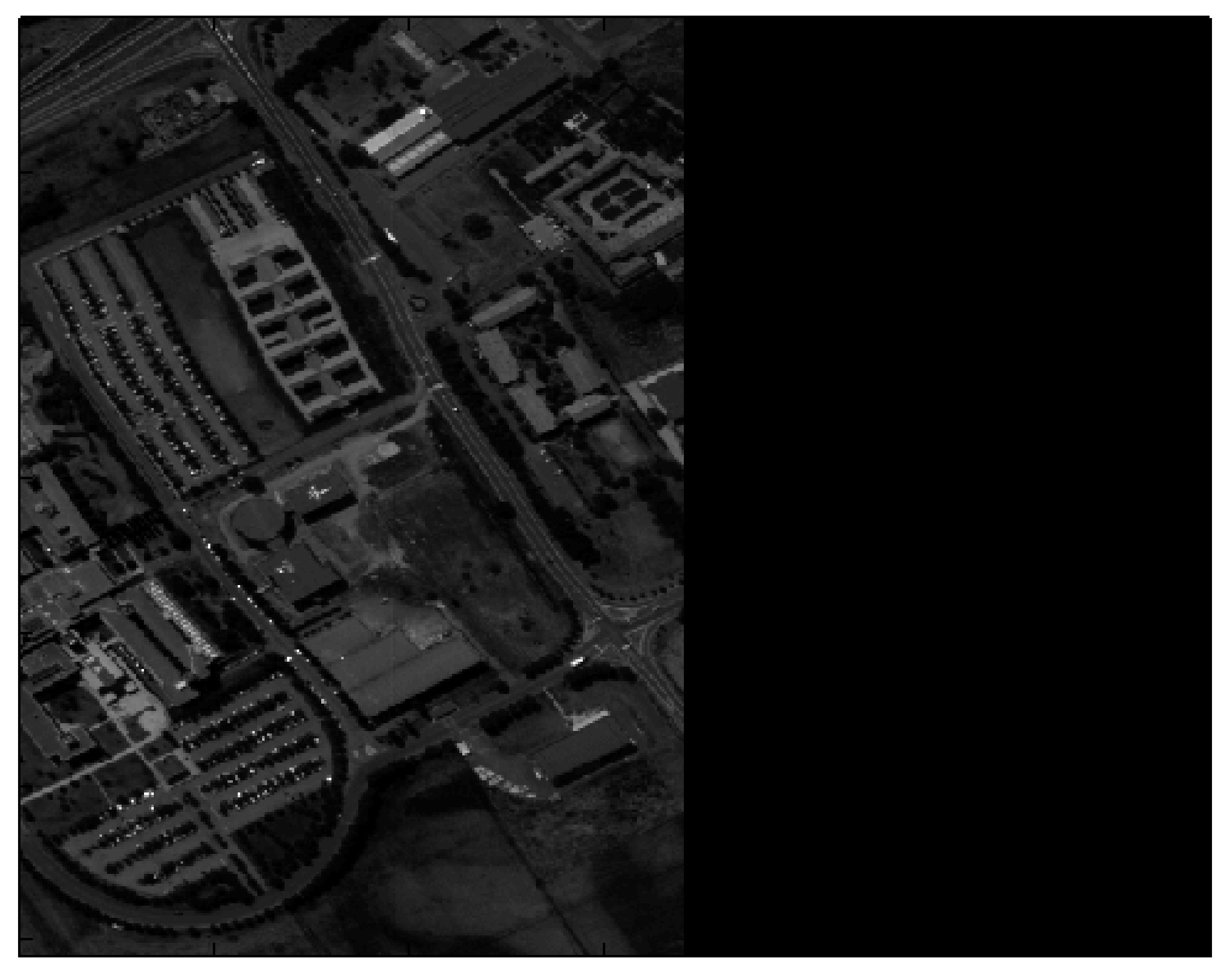
2.2.3. Pavia University Dataset

The Pavia University dataset was obtained by the ROSIS sensor in Pavia, northern Italy. The number of spectral bands in Pavia University is 103. The University of Pavia is 610 × 610 pixels and contains nine categories. Figure 3 shows the sample band of the Pavia University dataset.

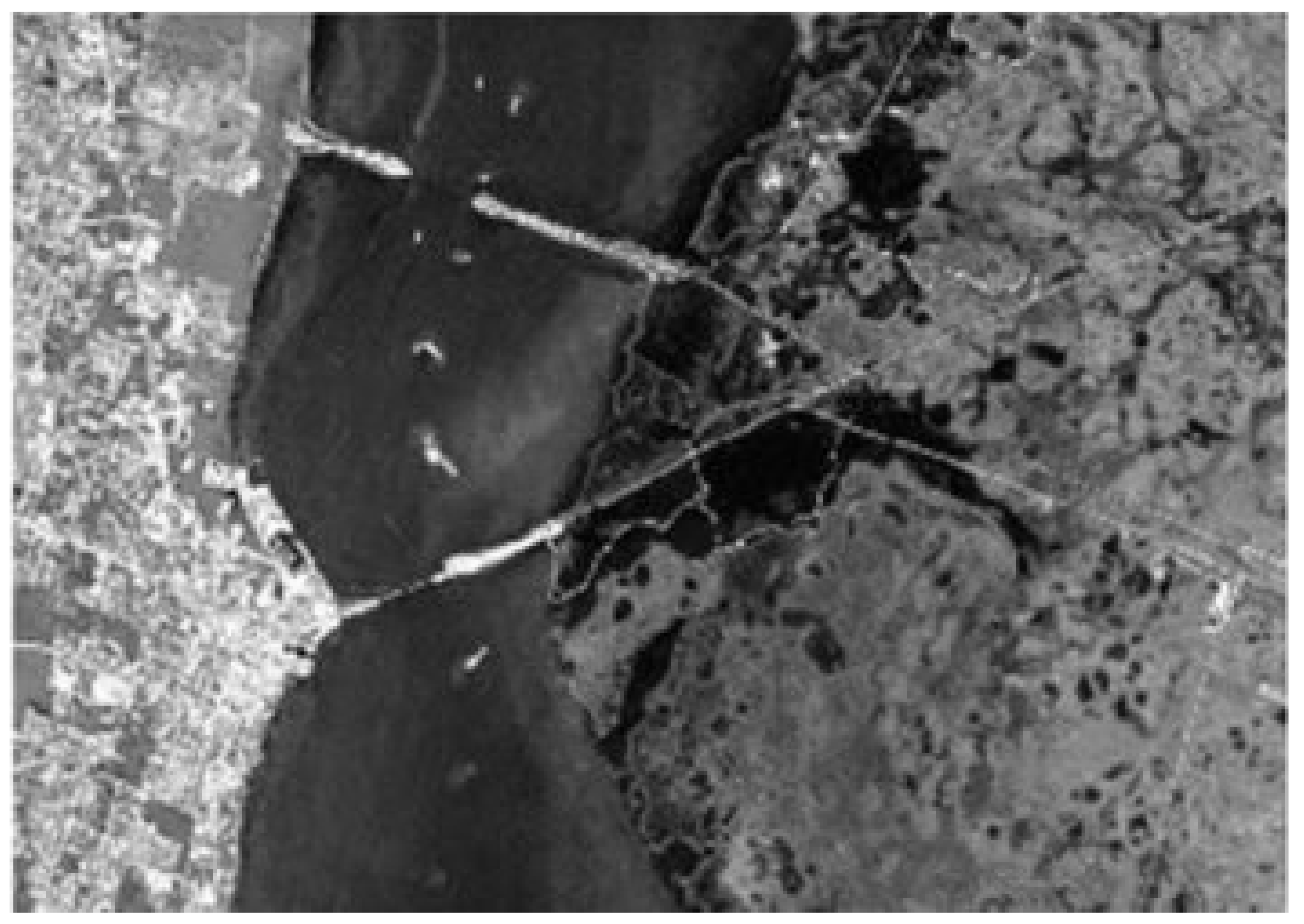
2.2.4. Kennedy Space Center Dataset

The Kennedy Space Center dataset was collected by AVIRIS over the Kennedy Space Center in Florida. The number of spectral bands is 224 and the pixel is 512 × 614. It contains 13 categories. Figure 4 shows the sample band of the Kennedy Space Center dataset.

2.3. Task

Support vector machines are widely used in hyperspectral image classification. However, the SVM classification mechanism assumes that the datasets are separable in parallel planes. For real hyperspectral image data, its data distribution makes it difficult to meet the property of being separable in parallel planes; therefore, using support vector machine classification means losing certain classification accuracy to a certain extent.

For the problem that the decision plane of support vector machine in hyperspectral image classification makes it difficult to conform to the trend of data distribution, this article proposes a classification method using non-parallel support vector machine to improve the support vector machine. Compared with SVMs, non-parallel SVMs have better decision hyperplane degrees of freedom. The classification hyperplane structure of the non-parallel SVM makes the decision plane more in line with the distribution trend of hyperspectral data, thus obtaining better classification accuracy than SVM.

2.4. Support Vector Machine

For the second-class classification of m data points in n dimensional feature space $R^n$, the matrix A is used to represent all data points by using $m\times n$, and the No. i data point is $A_i\left(i=1,2,\dots ,m\right)$, $A_i={\left(i=A_{i1},A_{i2},\dots ,A_{in}\right)}^T$. Let $y_i\in \left.\left\{1,-1\right.\right\}$ represent the category information to which the No. i data point belongs. The $m\times m$ diagonal matrix Y is established by using $y_i$ as diagonal line, that is, $Y_{ii}$ represents the category information to which the $A_i$ data point belongs.

First, consider the case of linear SVM, which looks for a classification hyperplane as follows:

$$f\left(x\right)={\omega }^T·x+b=0$$

(1)

Here, $\omega \in R^n$ and $b\in R^n$. The soft interval hinge loss function is introduced to measure the empirical risk. The SVM original optimization problem can be expressed as follows by introducing regularization term $\frac{1}{2}{\omega }^T\omega$ and relaxation variable $\xi =\left({\xi }_1,\dots ,{\xi }_m\right)$:

$$\begin{array}{c}\underset{\omega ,b,\zeta }{\min }\hspace{1em}\frac{1}{2}{\omega }^T\omega +{ \mathrm{Ce}}^T\xi \hfill \\ s.t.\hspace{1em}Y\left(A\omega + \mathrm{eb}\right)+\xi \ge e\hfill \\ \hfill \xi \ge 0.\end{array}$$

(2)

Here, $C>0$ is the penalty coefficient, and minimized regularization term $\frac{1}{2}{\omega }^T\omega$ is equivalent to the distance between the two maximized supporting hyperplanes, ${\omega }^T·x+b=1$ and ${\omega }^T·x+b=-1$ and the structural risk minimized principle is implemented for the original problem.

The dual problem obtained by Lagrange Multiplier Method is shown as follows:

$$\begin{array}{c}\underset{\alpha }{\max }\hspace{1em}-\frac{1}{2}{\alpha }^{T}YA{A}^{T}Y\alpha +e^T\alpha \hfill \\ s.t.\hspace{1em}{e}^{T}Y\alpha =0\hfill \\ \hfill 0\le \alpha \le \mathrm{Ce}\hfill \\ \hfill \left(\omega =A^{T}Y\alpha \right)\hfill \end{array}$$

(3)

The solution of Lagrange Multiplier and further solution can be obtained by solving the above dual problem. Further, the solution of $\omega ,b$ can be obtained. The new data points are classified by the following decision function.

$$f\left(x\right)=\mathrm{sgn}\left({\omega }^T·x+b\right)$$

(4)

For the nonlinear classification problem, it can be transformed into a linear classification problem in a certain dimensional feature space by nonlinear transformation, and the linear support vector machine can be learned in the high-dimensional feature space. It is specifically expressed as. Where, $\phi \left(x\right)$ represents a mapping of $x$ to a high-dimensional space. In the dual problem of linear support vector machine learning, the nonlinear support vector machine is obtained by using kernel function instead of inner product. The dual problem of nonlinear SVM is as follows:

$$\begin{array}{c}\underset{\alpha }{\max }\hspace{1em}-\frac{1}{2}{\alpha }^{T}YK\left(A{A}^T\right)Y\alpha +e^T\alpha \hfill \\ s.t.\hspace{1em}{e}^T\alpha Y=0\hfill \\ \hfill 0\le \alpha \le \mathrm{Ce}\hfill \end{array}$$

(5)

The decision function of nonlinear support vector machine is:

$$f\left(x\right)=\mathrm{sgn}\left({\alpha }^T{Y}^{T}K\left(A·x\right)+b\right)$$

(6)

2.5. Non-Parallel Support Vector Machine

AERM-NPSVM is the smallest square term of adding the positive and negative samples, respectively, on the basis of SVM, which adds additional empirical risk terms and obtains two quadratic programming [25] problems. Hyperplane obtained by solving two $K\left(x,y\right)=\phi \left(x\right)·\phi \left(y\right)$ quadratic programming problems shifts to the direction of the distribution trend of positive and negative samples, so that two non-parallel classification hyperplanes can be obtained.

The two non-parallel decision planes obtained by AERM-NPSVM are:

$$f\left(x\right)={\omega }_{+}x+b=1$$

(7)

$$f\left(x\right)={\omega }_{-}x+b=-1$$

(8)

where the optimization problem for the positive sample is as follows:

$$\begin{array}{c}\underset{\omega ,b,\xi }{\min }\hspace{1em}\frac{1}{2}{‖{\omega }_{+}‖}^2+\frac{c_1}{2}{\eta }_{+}{}^T{\eta }_{+}+{ c}_3{e}^T{\xi }_{+}\hfill \\ s.t. \hspace{1em}\hspace{1em}\hspace{1em}\hspace{1em} A{\omega }_{+}+e_{+}{b}_{+}={\eta }_{+}\hfill \\ \hfill Y\left(C{\omega }_{+}+ e{b}_{+}\right)+{\xi }_{+}\ge e\\ \hfill {\xi }_{+} \ge 0.\end{array}$$

(9)

The optimization problem for negative samples is as follows:

$$\begin{array}{c}\underset{\omega ,b,\xi }{\min }\hspace{1em}\frac{1}{2}{‖{\omega }_{-}‖}^2+\frac{c_2}{2}{\eta }_{-}{}^T{\eta }_{-}+{ c}_{{}_4}{e}^T{\xi }_{-}\hfill \\ s.t. \hspace{1em}\hspace{1em}\hspace{1em}\hspace{1em} B{\omega }_{-}+e_{-}{b}_{-}={\eta }_{-}\hfill \\ \hfill Y\left(C{\omega }_{-}+ e{b}_{-}\right)+{\xi }_{-} \ge e\\ \hfill {\xi }_{-} \ge 0.\end{array}$$

(10)

Here, A is a matrix of all positive sample points, B is a matrix of all negative sample points, C is a matrix of all sample points, m₊ represents the number of all positive samples, m₋ represents the number of all negative samples, m represents the number of all samples, ${\eta }_{+}$ and ${\eta }_{-}$ are m dimensional vector, ${\xi }_{+}$ and ${\xi }_{-}$ are slack variables and $c_i,i=1,2,3,4$ is penalty parameter. $e_{+}$ is the vector with a value of 1 with dimension of m₊, $e_{-}$ is a vector with a value of 1 with dimension of m₋ and $e$ is a vector with a value of 1 with dimension of m. Taking Formula (9) as an example, the term $\frac{1}{2}{‖{\omega }_{+}‖}^2$ minimizes the structural risk by maximizing the distance between the classification planes, and $c_3{e}^T{\xi }_{+}$ is the hinge loss function. These two constitute the original problem of the standard support vector machine; $\frac{1}{2}{\eta }_{+}^T{\eta }_{+}$ is the least square term of the positive sample. It adds an additional empirical risk minimization to the original problem of S, which shifts the classification hyperplane in the direction of the positive sample distribution trend, where c₁ measures the magnitude of this degree.

For the problems of (9) and (10), if the penalty parameters c₁ and c₂ are 0, we get the optimization problem of SVM; that is, the traditional SVM model is a special case of AERM-NPSVM in c₁ = c₂ = 0.

Solve the dual problem [26] by using the Lagrange Multiplier Method; the Lagrangian function of the original problem (9) is as follows:

$$\begin{array}{l}L\left({\omega }_{+},b_{+},\xi ,\alpha ,\beta ,\lambda \right)=\frac{1}{2}{‖{\omega }_{+}‖}^2+\frac{c_1}{2}{\eta }_{+}^T{\eta }_{+}^{}\\ +c_3{e}^T{\xi }_{+}+{\lambda }_{}^T\left(A{\omega }_{+}+e_{+}{b}_{+}-{\eta }_{+}^{}\right)\\ +{\alpha }_{}{}^T\left(e-\xi -Y\left(C{\omega }_{+}+e{b}_{+}\right)\right)-{\beta }_{}^T{\xi }_{+}\end{array}$$

(11)

Here, $\alpha =\left({\alpha }_1,\dots ,{\alpha }_m\right), \beta =\left({\beta }_1,\dots ,{\beta }_m\right)$ and $\lambda =\left({\lambda }_1,\dots ,{\lambda }_{m_{+}}\right)$ are the Lagrange multiplier vector. The KKT conditions for the partial derivatives of ${\omega }_{+},b_{+},{\xi }_{+},\alpha ,\beta ,\lambda$ in Lagrange functions (11) are as follows:

$${\nabla }_{{\omega }_{+}}L={\omega }_{+}+A^T\lambda -C^T{Y}^T\alpha =0$$

(12a)

$${\nabla }_{b_{+}}L=e_{+}{}^T\lambda -e^T{Y}^T\alpha =0$$

(12b)

$${\nabla }_{{\eta }_{+}}L=c_1{\eta }_{+}-\lambda =0$$

(12c)

$${\nabla }_{{\xi }_{+}}L=c_3{e}^T-{\alpha }^T-{\beta }^T=0$$

(12d)

$$Y\left(C{\omega }_{+}+e{b}_{+}\right)+{\xi }_{+}\ge e, {\xi }_{+}\ge 0$$

(12e)

$${\alpha }^T\left(e-{\xi }_{+}-Y\left(C{\omega }_{+}+e{b}_{+}\right)\right)=0, {\beta }^T{\xi }_{+}=0$$

(12f)

$$\alpha \ge 0, \beta \ge 0$$

(12g)

Because $\beta \ge 0$, it can be concluded that from (12d):

$$0\le \alpha \le c_3{e}^T$$

(13)

Bring (12a)–(12g) into the Lagrangian function (11) to get the dual formula, which is as follows:

$$\begin{array}{c}\underset{\alpha }{\max }{\hspace{1em}e}_{}^T\alpha -\frac{1}{2}\left[{\lambda }^T {\alpha }^T\right]\left[\begin{array}{cc}A{A}^T+\frac{1}{c_1}{I}_{+}& -A{C}^T{Y}^T\\ -YC{A}^T& YC{C}^T{Y}^T\end{array}\right]{\left[{\lambda }^T {\alpha }^T\right]}^T\hfill \\ s.t.\hspace{1em}\hspace{1em}\hspace{1em}\hspace{1em}{\left[e_{{}_{+}}^T -e^T{Y}^T\right]}^T {\left[{\lambda }^T {\alpha }^T\right]}^T=0\hfill \\ \hfill 0\le \alpha \le c_3{e}^T\hfill \end{array}$$

(14)

Here, $I_{+}$ is the unit matrix with dimension m₊. The dual Equation (14) is similar to the dual Equation (3) of the support vector machine. Solving the dual problem gives the solution to the original problem.

The optimal solution $\left[{\lambda }^{*},{\alpha }^{*}\right]$ is obtained by solving the above dual problem, and then the normal vector is obtained by the Formula (12a):

$${\omega }_{+}=-A^T{\lambda }_{{}_{}}^{*}+C^T{Y}^T{\alpha }_{}^{*}$$

(15)

Obtain from the formula of (12b) and (12c):

$$A{\omega }_{+}+e_{+}{b}_{+}={\eta }_{+}=\frac{1}{c_1}{\lambda }_{}^{*}$$

(16)

Equation (16) calculates the offset b+ of the positive class classification hyperplane by the average of all positive sample offsets, making the result more robust. It can be further concluded that the offset b+ is:

$$b_{+}=\frac{e_{{}_{+}}^T\left(-A{\omega }_{+}+\frac{1}{c_1}{\lambda }_{}^{*}\right)}{m_{+}}$$

(17)

Similarly, the dual formula of negative samples can be obtained as follows:

$$\begin{array}{c}\underset{\alpha }{\max }{\hspace{1em}e}_{}^T\alpha -\frac{1}{2}\left[{\theta }^T {\gamma }^T\right]\left[\begin{array}{cc}B{B}^T+\frac{1}{c_2}{I}_{-}& -B{C}^T{Y}^T\\ -YC{A}^T& YC{C}^T{Y}^T\end{array}\right]{\left[{\theta }^T {\gamma }^T\right]}^T\hfill \\ s.t.\hspace{1em}\hspace{1em}{\left[e_{{}_{-}}^T - e^T{Y}^T\right]}^T {\left[{\theta }^T {\gamma }^T\right]}^T=0\hfill \\ \hspace{1em}\hspace{1em}\hspace{1em}\hspace{1em} 0\le \gamma \le c_4{e}^T\hfill \end{array}$$

(18)

Here, $I_{-}$ is the unit matrix with dimension of m₋.

The optimal solution $\left[{\theta }^{*},{\gamma }^{*}\right]$ is obtained by solving the above dual problem, and the normal vector ${\omega }_{-}$ and offset $b_{-}$ are further solved.

$${\omega }_{-}=-B^T{\theta }_{}^{*}+C^T{Y}^T{\gamma }_{}^{*}$$

(19)

$$b_{{}_{-}}=\frac{e_{{}_{-}}^T\left(-B{\omega }_{{}_{-}}+\frac{1}{c_2}{\gamma }_{}^{*}\right)}{m_{{}_{-}}}$$

(20)

By comparing the distance between the data point and the two hyperplanes, we can judge which category it should belong to. $b_{+}=b_{+}-1$, $b_{-}=b_{-}+1$. The decision function can be written as follows:

$$\mathrm{Class} = \arg \underset{i=+,-}{\min }\hspace{1em}\frac{\left|\left(x_{}^T·{\omega }_i\right)+{ b}_i\right|}{‖{\omega }_i‖}$$

(21)

Here, $\left|·\right|$ is an absolute value operation and $‖·‖$ is a two-norm operation.

The above only illustrates the linear case of the AERM-NPSVM model. Because the derivation of the formula is too complicated, please refer to the Appendix A.1 for the description of the nonlinear situation. Furthermore, the BC-AERM-NPSVM algorithm is an improvement over the AERM-NPSVM algorithm. It makes the offset have a unique value, makes the solution of the offset easier. The dual problem has no equality constraints, which makes the solution algorithm better and more diverse. See the Appendix A.2 for details. Both AENSVM and AEBNSVM, proposed above, are binary classification models, which cannot directly classify multi-class hyperspectral datasets. AENSVM and AEBNSVM are used in the same way on hyperspectral datasets. The following uses AENSVM as an example to illustrate how to classify hyperspectral images. The specific application method is shown in Algorithm 1.

Algorithm 1. The classification process of the AENSVM algorithm model on the hyperspectral dataset.

Step 1: Combining each category of the hyperspectral dataset in pairs is used to obtain $\frac{1}{2}\left(n\times \left(n-1\right)\right)$ binary classification tasks.

Step 2: Set the hyperparameters c1, c2, c3, c4 of the AENSVM model.

Step 3: Each binary classification task is trained using AENSVM.   1. Use the parameters set in Step 2 to solve the parameters ${\alpha }^{*},{\lambda }^{*},{\theta }^{*},{\gamma }^{*}$ according to Formulas (14) and (18).   2. The offsets of the two decision hyperplanes are obtained by (17) and (20).   Finally, $\frac{1}{2}\left(n\times \left(n-1\right)\right)$ classifier models are obtained.

Step 4: For the $\frac{1}{2}\left(n\times \left(n-1\right)\right)$ classifier models trained in Step 3, the category of the new sample is predicted by Formula (30), all predicted categories are recorded, and the sample is classified into the category with the most votes by voting.

2.6. Accuracy Assessment

Confusion matrix is often used in classification performance evaluation in the form of:

$$H=\left[\begin{array}{cccc}{h}_{11}& h_{12}& \cdots & h_{1N}\\ h_{21}& h_{22}& \cdots & h_{2N}\\ ⋮& ⋮& & ⋮\\ h_{N1}& h_{N2}& \cdots & h_{NN}\end{array}\right]$$

(22)

The overall classification accuracy (OA) and Kappa coefficient (Kappa) derived from the confusion matrix are used as important evaluation indexes of classification. Although the OA value can well represent the classification accuracy, for multi-category features with extremely unbalanced number of category pixels, its value is greatly affected by the category with more pixel data and cannot well represent the features of each category. The Kappa coefficient comprehensively considers various factors in the confusion matrix and can comprehensively reflect the accuracy of the overall classification. The larger the value of the kappa coefficient, the higher the accuracy of the corresponding classification algorithm. Therefore, the OA and Kappa coefficients are usually used to jointly evaluate the classification accuracy of hyperspectral images.

3. Results

This part shows the classification performance comparison of SVM, TWSVM, AENSVM and AEBNSVM under the four hyperspectral datasets of Salinas-A, Pavia Center, Pavia University and Kennedy Space Center. All the classification algorithms are carried out in a nonlinear way by using Gaussian kernel functions.

The division of training test set of Salinas-A is shown in

Table 1. Ground truth classes for the Salinas-A scene and their respective samples number.

Class	Samples	Train	Test
Brocoli_green_weeds_1	391	39	352
Corn_seesced_green_weeds	1343	134	1109
Lettuce_romaine_4wk	616	61	555
Lettuce_romaine_5wk	1525	152	1373
Lettuce_romaine_6wk	674	67	607

.

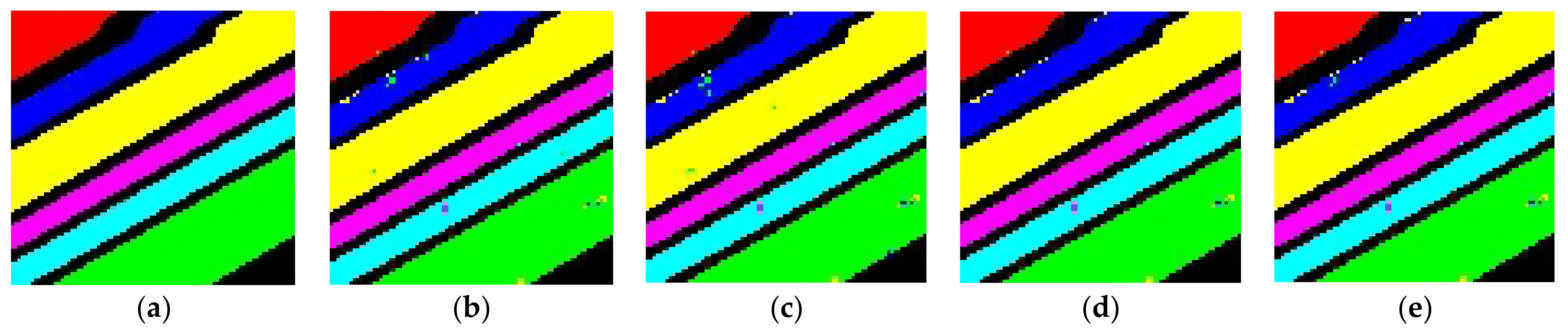
3.1. Salinas-A Dataset

Figure 5b–e are the recovery graphs of the prediction results of Salinas-A data using SVM, TWSVM, AENSVM and AENBSVM, respectively. If you look closely, you can see that the classification accuracy of AENSVM and AENBSVM has improved compared to SVM. The classification accuracy of each category is shown in Figure 6, and Figure 5 is analyzed in detail through Figure 6. AENSVM and AEBNSVM achieve 0.08%, 0.92% and 0.16% accuracy improvement over SVM on Corn_senesced_green_weeds, Lettuce_romaine_4wk and Lettuce_romaine_6wk categories, respectively, where TWSVM has 1.11% better accuracy over SVM in the Lettuce_romaine_4wk category. AENSVM and AEBNSVM can balance empirical risk minimization and structural risk minimization by adjusting parameters c₁ and c₃. The classification results of TWSVM show that empirical risk minimization can make the Lettuce_romaine_4wk classification effect better. AENSVM and AEBNSVM also achieve better results than SVM by adjusting the degree of empirical risk minimization, and the characteristics of structural risk minimization also ensure the accuracy of other categories. As in the Lettuce_romaine_5wk category, the classification accuracy of SVM, AENSVM and AEBNSVM is 0.22% higher than that of TWSVM. It can be seen from

Table 2. Classification results of Salinas-A hyperspectral images.

Experimental Method	SVM	TWSVM	AENSVM	AEBNSVM
OA	99.29	99.11	99.43	99.43
Kappa	99.12	98.91	99.30	99.30

that the difficulty of Salinas-A classification is low, and SVM, TWSVM, AENSVM and AEBNSVM all get more than 99% classification accuracy. The overall classification accuracy of AENSVM and AEBNSVM is 0.14% higher than SVM and 0.32% higher than TWSVM, the Kappa coefficient is 0.18% higher than SVM and 0.39% higher than TWSVM.AENSVM; AEBNSVM non-parallel support vector machines are more suitable for data distribution under the premise of good SVM properties, so they get better experimental results.

The division of training test set of Pavia Center is shown in

Table 3. Ground truth classes for the Pavia Center scene and their respective numbers of samples.

Class	Samples	Train	Test
Water	65,971	300	65,671
Trees	7598	300	7298
Asphalt	3090	300	2790
Self-Blocking Bricks	2685	300	2385
Bitumen	6584	300	6284
Tiles	9248	300	8948
Shadows	7287	300	6987
Meadows	42,826	300	42,526
Bare Soil	2863	300	2563

.

3.2. Pavia Center Dataset

Figure 7b–e are the recovery results of the Pavia Center data predicted by SVM, TWSVM, AENSVM and AENBSVM, respectively. Figure 8 shows the classification accuracy of each category in Figure 7 in detail. On the Tree, Self-Blocking Bricks, Bitumen, Tiles, Shadows and Meadows categories, the classification accuracy of AENSVM and AEBNSVM is 0.25%, 0.67%, 0.46%, 0.22%, 0.41% and 0.58% higher than SVM, respectively. The classification accuracy of TWSVM is 0.86%, 2.98%, 0.44% and 0.53% higher than that of SVM in the categories of Tree, Self-Blocking Bricks, Tiles and Meadows, respectively. The classification accuracy of Bitumen and Shadows categories is reduced by 0.35% and 1.71%, respectively. It can be seen that the classification results of TWSVM on Tree, Self-Blocking Bricks and Tiles categories are better, indicating that these categories can obtain better classification accuracy when the proportion of empirical risk minimization is high. However, it can be seen from

Table 4. Classification results of Pavia Center hyperspectral images.

Experimental Method	SVM	TWSVM	AENSVM	AEBNSVM
OA	98.33	98.25	98.50	98.50
Kappa	97.62	97.50	97.86	97.86

that the overall classification accuracy of TWSVM is 0.08% lower than that of SVM, and the kappa coefficient is 0.12% lower than that of SVM. In order not to affect the overall accuracy, the empirical risk minimization terms of AENSVM and AEBNSVM cannot be weighted too high, so the classification accuracy of TWSVM cannot be achieved on these categories. On the Asphalt category, the classification accuracy of AENSVM and AEBNSVM is 0.22% lower than that of SVM, and the classification accuracy of TWSVM is 2.44% lower than that of SVM. It can be seen that increasing the weight of empirical risk minimization will reduce the classification accuracy of the Asphalt category, but in order to make the overall classification accuracy higher, the classification accuracy of this category is traded off. From the overall classification accuracy in Table 4, it can be seen that the classification accuracy of AENSVM and AEBNSVM is 0.25% higher than that of SVM, and the kappa coefficient is 0.36% higher than that of SVM. AENSVM and AEBNSVM still have higher kappa coefficients on the premise of higher accuracy, confirming their effectiveness in adding an additional empirical risk minimization term.

The division of training test set of Pavia University is shown in

Table 5. Ground truth classes for the Pavia University scene and their respective numbers of samples.

Class	Samples	Train	Test
Asphalt	6631	300	6331
Meadows	18,649	300	18,349
Gravel	2099	300	1790
Trees	3064	300	2764
Painted metal sheets	1345	300	1045
Bare Soil	5029	300	4729
Bitumen	1330	300	1030
Self-Blocking Bricks	3682	300	3382
Shadows	947	300	647

.

3.3. Pavia University Dataset

Figure 9b–e are the recovery graphs of the prediction results of Pavia University data using SVM, TWSVM, AENSVM and AENBSVM, respectively. It can be seen that the prediction results of AENSVM and AENSVM are better in some categories. Figure 10 shows the classification accuracy of each category in Figure 9 in detail, followed by a detailed analysis of Figure 10. AENSVM and AEBNSVM have the same weights for the additional empirical risk minimization term added when all categories are classified during parameter tuning. This behavior will produce better or worse results for the classification accuracy of a single category than SVM. Take Meadows and Bare Soil as the two more representative categories to illustrate. For the Meadows category, the classification accuracy of AENSVM and AEBNSVM is 2.88% higher than that of SVM, indicating that the additional empirical risk minimization term under the current weights improves the classification accuracy of the Meadows category. For the Soil category, the classification accuracy of AENSVM and AEBNSVM is 2.95% lower than that of SVM, indicating that the additional empirical risk minimization under the current weights has a detrimental effect on the Soil category. However, from the overall classification accuracy in

Table 6. Classification results of Pavia University hyperspectral images.

Experimental Method	SVM	TWSVM	AENSVM	AEBNSVM
OA	91.49	91.53	92.53	92.43
Kappa	88.76	88.77	90.05	89.92

, the classification accuracy of AENSVM and AEBNSVM has better performance than that of standard SVM and TWSVM. The accuracy of AENSVM is 1.05% higher than that of standard SVM, and the Kappa coefficient is 1.29% higher than that of SVM. The accuracy of AEBNSVM is 0.95% higher than that of standard SVM, and the Kappa coefficient is 1.16% higher than that of SVM. This shows that although the additional empirical risk minimization makes the classification results of some single categories worse than SVM, it can achieve better classification results as a whole. The effectiveness of AENSVM and AENBSVM on the multi-classification problem of hyperspectral remote sensing images is demonstrated.

The division of training test set of Kennedy Space Center is shown in

Table 7. Sample information for the Kennedy Space Center dataset.

Class	Samples	Train	Test
Scrub	761	200	561
Willow swamp	243	194	49
CP hammock	256	200	56
Slash pine	252	200	52
Oak/Broadleaf	161	128	33
Hardwood	229	184	45
Swamp	105	84	21
Graminoid marsh	431	200	231
Spartina marsh	520	200	320
Cattail marsh	404	200	204
Salt marsh	419	200	219
Mud flats	503	200	303
Water	527	200	327

.

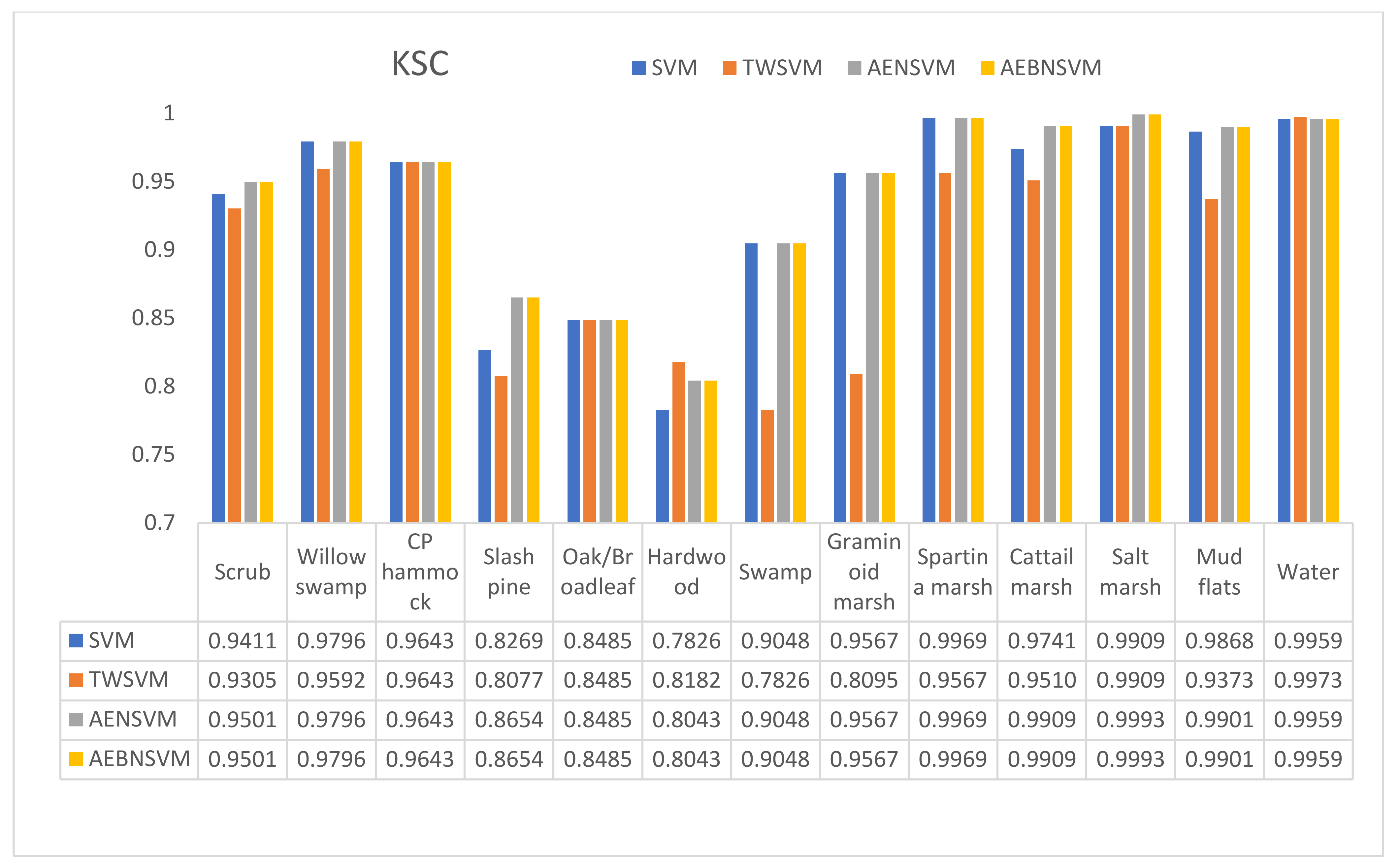
3.4. Kennedy Space Center Dataset

Figure 11b–e are the recovery charts of the Kennedy Space Center data using SVM, TWSVM, AENSVM and AENBSVM, respectively. Figure 12 shows the classification accuracy of each category in Figure 11 in detail. It can be seen that the classification accuracy of TWSVM, which only performs empirical risk minimization, is 3.56% higher than that of SVM on the Hardwood class, and the classification accuracy of the other classes is generally poor. For example, on the Swamp, Graminoid marsh and Spartina marsh categories, the classification accuracy of TWSVM is 12.22%, 14.72 and 4.02% lower than that of SVM, respectively. It can be seen from the data that in the case of fewer samples and more categories, the classification performance of TWSVM is worse than that of SVM. It can be seen from

Table 8. Classification results of Kennedy Space Center hyperspectral images.

Experimental Method	SVM	TWSVM	AENSVM	AEBNSVM
OA	96.78	95.39	96.95	96.95
Kappa	96.22	94.72	96.51	96.51

that the overall classification accuracy of TWSVM is 1.39% lower than that of SVM. Kappa coefficient is 1.5% lower than SVM. AENSVM and AENBSVM inherit the structural risk minimization property of SVM, and at the same time, by adjusting the weight of the empirical risk minimization term, the classification accuracy is improved to a certain extent. For example, on the Scrub, Slash pine and Hardwood categories, AENSVM and AEBNSVM improve the classification accuracy by 0.9%, 3.85% and 2.17%, respectively, over SVM. From Table 8, the overall accuracy of AENSVM and AEBNSVM is 0.17% and 0.29% higher than SVM, respectively. This confirms the effectiveness of AENSVM and AENBSVM on the multi-classification problem of hyperspectral remote sensing images.

The experimental results on the above four datasets demonstrate the applicability of the AENSVM and AENBSVM algorithms under different datasets.

4. Conclusions

As a traditional excellent classification tool, SVM has excellent performance in hyperspectral image classification. At present, most of the SVM models are based on parallel distribution boundaries, but this premise is not consistent with the actual situation. Although TWSVM breaks this premise, its classification effect is still not very satisfactory. The fundamental reason is that it only minimizes the empirical risk, so its generalization ability is relatively poor, and it does not obtain a better classification result than SVM in the experiment. The non-parallel structure of AEBNSVM and AENSVM proposed in this article has better classification results than the parallel structure of SVM. First of all, it adds the empirical risk minimization term on the basis of SVM to obtain two non-parallel hyperplanes and classifies them by way of non-parallel planes. Compared with the SVM classification effect of parallel structures, it has a certain improvement. Furthermore, it has the excellent property of structural risk minimization of parallel structure SVM, so its generalization ability of TWSVM is stronger than that of the non-parallel structure. For the algorithm proposed in this article, the premise is that the hyperspectral data distribution does not follow the trend of being separable in parallel planes. When the hyperspectral data distribution conforms to the parallel plane distribution trend, the algorithm proposed in this article is similar to the SVM in classification accuracy, but the scale of the problem is more complicated. Therefore, the algorithm in this article is more effective when it is difficult to classify the hyperspectral data distribution parallel decision plane.

In the experiments performed in this article, the classification of all hyperspectral images only uses its spectral information, and the classification accuracy is not high, compared with the current popular deep learning classification methods. It should be noted that the main purpose of this article is to improve the performance of the traditional parallel structure SVM by proving the effectiveness of the proposed non-parallel structure of SVM. In the future, we will discuss the double-layer structure and even deep structure of SVM on the basis of spatial information and spectral information fusion, combined with the non-parallel structure proposed in this article, in order to further improve the classification accuracy of SVM.

References

1. Zhong, Y.; Wang, X.; Wang, S.; Zhang, L. Advances in spaceborne hyperspectral remote sensing in China. Geo-Spat. Inf. Sci. 2021, 24, 95–120. [Google Scholar] [CrossRef]
2. Lu, B.; Dao, P.D.; Liu, J.; He, Y.; Shang, J. Recent advances of hyperspectral imaging technology and applications in agriculture. Remote Sens. 2020, 12, 2659. [Google Scholar] [CrossRef]
3. Stein, D.W.; Beaven, S.G.; Hoff, L.E.; Winter, E.M.; Schaum, A.P.; Stocker, A.D. Anomaly detection from hyperspectral imagery. IEEE Signal Processing Mag. 2002, 19, 58–69. [Google Scholar] [CrossRef] [Green Version]
4. Li, J.; Pei, Y.; Zhao, S.; Xiao, R.; Sang, X.; Zhang, C. A review of remote sensing for environmental monitoring in China. Remote Sens. 2020, 12, 1130. [Google Scholar] [CrossRef] [Green Version]
5. Tan, K.; Du, P. Hyperspectral Remote Sensing Image Classification Based on Support Vector Machine. J. Infrared Millim. Waves 2008, 27, 123–128. [Google Scholar] [CrossRef]
6. Wang, Y. Remote Sensing Image Automatic Classification with Support Vector Machine. Comput. Simul. 2013, 30, 378–385. [Google Scholar]
7. Lv, W.; Wang, X. Overview of Hyperspectral Image Classification. J. Sens. 2020, 2020, 13. [Google Scholar] [CrossRef]
8. Song, W.; Li, S.; Kang, X.; Huang, K. Hyperspectral image classification based on KNN sparse representation. In Proceedings of the 2016 IEEE International Geoscience and Remote Sensing Symposium (IGARSS), Beijing, China, 10–15 July 2016; pp. 2411–2414. [Google Scholar] [CrossRef]
9. Goel, P.K.; Prasher, S.O.; Patel, R.M.; Landry, J.A.; Bonnell, R.B.; Viau, A.A. Classification of hyperspectral data by decision trees and artificial neural networks to identify weed stress and nitrogen status of corn. Comput. Electron. Agric. 2003, 39, 67–93. [Google Scholar] [CrossRef]
10. Pradhan, B. A comparative study on the predictive ability of the decision tree, support vector machine and neuro-fuzzy models in landslide susceptibility mapping using GIS. Comput. Geosci. 2013, 51, 350–365. [Google Scholar] [CrossRef]
11. Melgani, F.; Bruzzone, L. Classification of hyperspectral remote sensing images with support vector machines. IEEE Trans. Geosci. Remote Sens. 2004, 42, 1778–1790. [Google Scholar] [CrossRef] [Green Version]
12. Cortes, C.; Vapnik, V. Support-vector networks. Mach. Learn. 1995, 20, 273–297. [Google Scholar] [CrossRef]
13. Sain, S.R. The Nature of Statistical Learning Theory; Taylor & Francis: Abingdon, UK, 1996; p. 409. [Google Scholar]
14. Zhang, D.; Zhou, Z.H.; Chen, S. Semi-supervised dimensionality reduction. In Proceedings of the 2007 SIAM International Conference on Data Mining. Society for Industrial and Applied Mathematics, Minneapolis, MN, USA, 26–28 April 2007; pp. 629–634. [Google Scholar]
15. Harikiran, J.J. Hyperspectral image classification using support vector machines. IAES Int. J. Artif. Intell. 2020, 9, 684. [Google Scholar] [CrossRef]
16. Mangasarian, O.L.; Wild, E.W. Multisurface proximal support vector machine classification via generalized eigenvalues. IEEE Trans. Pattern Anal. Mach. Intell. 2005, 28, 69–74. [Google Scholar] [CrossRef] [PubMed]
17. Khemchandani, R.; Chandra, S. Twin support vector machines for pattern classification. IEEE Trans. Pattern Anal. Mach. Intell. 2007, 29, 905–910. [Google Scholar]
18. Schölkopf, B.; Smola, A.J.; Bach, F. Learning with Kernels: Support Vector Machines, Regularization, Optimization, and Beyond; MIT Press: Cambridge, MA, USA, 2002. [Google Scholar]
19. Zhang, C.; Tian, Y.; Deng, N. The new interpretation of support vector machines on statistical learning theory. Sci. China Ser. A Math. 2010, 53, 151–164. [Google Scholar] [CrossRef]
20. Kaya, G.T.; Torun, Y.; Küçük, C. Recursive feature selection based on non-parallel SVMs and its application to hyperspectral image classification. In Proceedings of the 2014 IEEE Geoscience and Remote Sensing Symposium, Quebec City, QC, Canada, 13–18 July 2014; pp. 3558–3561. [Google Scholar]
21. Liu, Z.; Zhu, L. A novel remote sensing image classification algorithm based on multi-feature optimization and TWSVM. In Proceedings of the Ninth International Conference on Digital Image Processing (ICDIP 2017). International Society for Optics and Photonics, Hong Kong, China, 19–22 May 2017. [Google Scholar]
22. Wang, L.; Lu, T.; Yang, Y. Least Squares Twin Support Vector Machines Based on Sample Reduction for Hyperspectral Image Classification. In Proceedings of the International Conference on Advances in Mechanical Engineering and Industrial Informatics (AMEII 2015), Zhengzhou, China, 11–12 April 2015. [Google Scholar]
23. Wang, L.; Du, X. Semi-supervised classification of hyperspectral images applying the combination of K-mean clustering and twin support vector machine. Appl. Sci. Technol. 2017, 44, 12–18. [Google Scholar]
24. Okwuashi, O.; Ndehedehe, C.E. Deep support vector machine for hyperspectral image classification. Pattern Recognit. 2020, 103, 107298. [Google Scholar] [CrossRef]
25. Kuhn, H.W.; Tucker, A.W. Nonlinear programming. In Traces and Emergence of Nonlinear Programming; Springer: Berlin/Heidelberg, Germany, 2014; pp. 247–258. [Google Scholar]
26. Tian, Y.; Ju, X.; Qi, Z.; Shi, Y. Improved twin support vector machine. Sci. China Math. 2014, 57, 417–432. [Google Scholar] [CrossRef]
Figure 1. Sample band of Salinas-A dataset.
Remotesensing 14 02447 g001
Figure 2. Sample band of Pavia Center dataset.
Remotesensing 14 02447 g002
Figure 3. Sample band of Pavia University dataset.
Remotesensing 14 02447 g003
Figure 4. Sample band of P Kennedy Space Center dataset.
Remotesensing 14 02447 g004
Figure 5. Salinas-A hyperspectral image classification result image. (a) (ground truth), (b) SVM, (c) TWSVM, (d) AENSVM, (e) AEBNSVM.
Remotesensing 14 02447 g005
Figure 6. Classification results of different categories of Salinas-A hyperspectral images.
Remotesensing 14 02447 g006
Figure 7. Pavia Center hyperspectral image classification result image. (a) (ground truth), (b) SVM, (c) TWSVM, (d) AENSVM, (e) AEBNSVM.
Remotesensing 14 02447 g007
Figure 8. Classification results of different categories of Pavia Center hyperspectral images.
Remotesensing 14 02447 g008
Figure 9. Pavia University hyperspectral image classification result image. (a) (ground truth), (b) SVM, (c) TWSVM, (d) AENSVM, (e) AEBNSVM.
Remotesensing 14 02447 g009
Figure 10. Classification results of different categories of Pavia University hyperspectral images.
Remotesensing 14 02447 g010
Figure 11. Kennedy Space Center hyperspectral image classification result image. (a) (ground truth), (b) SVM, (c) TWSVM, (d) AENSVM, (e) AEBNSVM.
Remotesensing 14 02447 g011
Figure 12. Classification results of different categories of Kennedy Space Center hyperspectral images.
Remotesensing 14 02447 g012