Abstract
Satellite data provide high potential for estimating crop yield, which is crucial to understanding determinants of yield gaps and therefore improving food production, particularly in sub-Saharan Africa (SSA) regions. However, accurate assessment of crop yield and its spatial variation is challenging in SSA because of small field sizes, widespread intercropping practices, and inadequate field observations. This study aimed to firstly evaluate the potential of satellite data in estimating maize yield in intercropped smallholder fields and secondly assess how factors such as satellite data spatial and temporal resolution, within-field variability, field size, harvest index and intercropping practices affect model performance. Having collected in situ data (field size, yield, intercrops occurrence, harvest index, and leaf area index), statistical models were developed to predict yield from multisource satellite data (i.e., Sentinel-2 and PlanetScope). Model accuracy and residuals were assessed against the above factors. Among 150 investigated fields, our study found that nearly half were intercropped with legumes, with an average plot size of 0.17 ha. Despite mixed pixels resulting from intercrops, the model based on the Sentinel-2 red-edge vegetation index (VI) could estimate maize yield with moderate accuracy (R2 = 0.51, nRMSE = 19.95%), while higher spatial resolution satellite data (e.g., PlanetScope 3 m) only showed a marginal improvement in performance (R2 = 0.52, nRMSE = 19.95%). Seasonal peak VI values provided better accuracy than seasonal mean/median VI, suggesting peak VI values may capture the signal of the dominant upper maize foliage layer and may be less impacted by understory intercrop effects. Still, intercropping practice reduces model accuracy, as the model residuals are lower in fields with pure maize (1 t/ha) compared to intercropped fields (1.3 t/ha). This study provides a reference for operational maize yield estimation in intercropped smallholder fields, using free satellite data in Southern Malawi. It also highlights the difficulties of estimating yield in intercropped fields using satellite imagery, and stresses the importance of sufficient satellite observations for monitoring intercropping practices in SSA.
1. Introduction
The sustainability of crop production in Sub-Saharan Africa (SSA) is threatened by several pressures, such as population growth [1], land degradation [2], pests [3], droughts [4], flooding, and climate change [5,6]. Smallholder agriculture accounts for 85% of the total farming area in SSA, but quantitative information on crop yield remains either poorly measured [7] or available at a very coarse spatial scale [8]. Due to the lack of reliable crop yield data, it is challenging to implement evidence-based policies and intervention programs to close yield gaps [7,9]. Routine and cost-effective estimates of crop yield are needed to address these challenges [7,9]. Particularly, efficient and spatially explicit mapping of yield is needed to better target sustainable intensification interventions [10], as relying on traditional field-based yield estimation is time-consuming and difficult to scale to large areas [7].
Earth observation (EO) data have been demonstrated to estimate crop yield at the field, country, and continental scales [11,12,13]. Progress has been made to assess within-field yield variability in smallholder farms [14], particularly with the new development of EO systems that offer increased revisit frequencies and increased spatial resolutions, such as Sentinel-2 data with 5-days revisit frequency at 10 m spatial resolution and daily PlanetScope data at 3 m. Empirical relationships between crop yield and vegetation indices (VIs) or biophysical variables (i.e., leaf area index—LAI), have been used for yield estimation in large homogeneous crop plots [15,16,17]; however, there are limited studies focusing on smallholder fields in SSA [18,19]. Linear empirical models are commonly used to estimate crop yields, although they are known to be site and crop-specific [10,20,21]. The linear models are, however, easy to develop and, thus, are particularly useful for operational purposes of agricultural monitoring services [20,21].
Several projects and platforms have been developed to utilize EO data for monitoring crop conditions and crop response to adverse environmental conditions, such as insects and droughts [22,23,24]. Such monitoring services are particularly crucial for SSA [21] in order to implement food-aid programs and take prompt mitigation strategies in the case of crop failure. They are usually implemented for large areas and rely on models that are rarely calibrated for specific regions and agricultural practices [22]. In SSA smallholder fields, EO data has been used to monitor crop conditions in response to droughts, but model performance and accuracy have not been evaluated [22]. Studies that have attempted to estimate crop yield at the field scale in SSA smallholder fields by using EO data are rather limited. For example, existing studies span only four countries (e.g., Burkina Faso, Kenya, Mali, and Uganda) and cover a subset of crop types cultivated across SSA (e.g., maize, wheat, and millet, sorghum, beans, and cotton) [7,10,18,25,26,27]. As such, they provide only a limited understanding of the potential of EO data for yield estimation in SSA.
Of the limited number of previous studies, few measured crop yield at the field scale [18,27,28,29]; instead, the majority of these studies rely on official crop yield statistics that are either available at the scale of administrative zones [8,30] or are desk-based yield estimates that are not always reliable [28,31]. In situ yield measurements are particularly scarce in SSA smallholder fields, thus limiting the accuracy of EO-based empirical models. It is recognized that the availability of reliable and sufficient in situ data would quickly accelerate progress in yield estimation in SSA (Burke et al., 2021). In addition, it is suggested that the accuracy of EO-based operational programs, such as global famine early warning [29] and agricultural monitoring systems [32], can be further improved when calibrated by using in situ data, particularly for the SSA region [22].
In addition to lack of reliable in situ yield data, other challenges associated with EO-based yield estimation in SSA include (1) frequent cloud contamination of optical satellite data; (2) limited spatial resolutions that fail to adequately represent the heterogeneous landscape [21] and small fields, which are particularly widespread in SSA as 80% of smallholders’ fields are smaller than 2 ha [33]; and (3) widely practiced intercropping that results in mixed satellite image pixels. All of these factors play a key role in determining the performance of EO-based empirical models. To address the first factor, temporal aggregation methods (i.e., temporal mean, maximum, and median) and high-temporal-resolution EO are needed. To address the second factor, satellite data providing a sufficient number of measurements relative to the field size (enabling within-field variation to be captured) are necessary, though there are trade-offs in terms of optimal spatial resolution and financial and computational costs. In addition, the landscape heterogeneity is correlated to environmental conditions and resources (i.e., water and nutrition) available for crops to grow, which can be reflected by the harvest index. In terms of the third factor (intercropping practices), legumes are commonly intercropped in maize fields that dominate most smallholder farming [34,35], while maize is the main staple food that grows in 97% of farming households in Southern Africa [36]. The intercropping practice poses difficulties for estimating both maize and intercrop yield using EO data. Therefore, field investigation of intercropping practices is critical for assessing how they may affect maize-yield estimation accuracy.
The aim of this paper is to understand opportunities and challenges in estimating crop yield in smallholder farming systems, using the currently available optical EO data. In particular, this study explored how reliable PlanetScope and Sentinel-2 EO data can be used to estimate maize yield in intercropped smallholder fields in Southern Malawi. We collected in situ data on crop field characteristics (e.g., field size, intercropping practices, yield, biomass, harvest index, and LAI) from 150 maize-dominated fields in 2019/2020 seasons. We used these data to calibrate and validate empirical EO-based models and assessed how the abovementioned factors, including spatial resolution/temporal aggregation of EO data, field size, within-field variability, harvest index and intercropping practices, affect the performance of the final maize-yield estimation.
2. Data and Methods
2.1. Study Area Description
Malawi is ranked as a low-income developing country in SSA, with around 90% of the population reliant on rain-fed subsistence smallholder farming [37]. Maize is the dominant crop type cultivated by over 97% of households [36]. Intercropping practices are common in maize fields, with one or more intercrops such as pigeon peas, soybeans, groundnuts, beans, and pumpkins [38] grown together on the same ground for all or most of the life cycle. The extent of individual smallholder fields is small, with an average of 0.32 ha in 2016, based on integrated household surveys [39]. The country is divided into three administrative regions, i.e., Southern, Central, and Northern regions. The Southern region is the most populated and has the majority of cropland generally characterized by smaller plot size than the other two regions. The Southern region is characterized by semi-arid conditions and has experienced climatic hazards, including droughts and dry spells, and localized floods in the past decades [40]. The rainy season, spanning from November to April, represents the main agricultural season in the majority of the country. In this study, in situ data collection was undertaken over maize-dominated fields in the Southern region, in the three Extension Planning Areas (EPAs) of Naminjiwa, Tamani, and Waruma, located in Phalombe District (Figure 1). In these areas, maize planting starts around November, and harvesting starts in March.
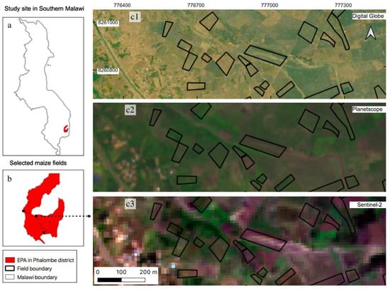
Figure 1.
Location of study sites on top of multi-source satellite images; (a) location of study sites showing three EPAs (red polygons) in Southern Malawi; (b) location of investigated maize (black outlines) within the study sites; (c1–c3) examples of selected maize fields on top of different satellite imagery: (c1): Digital Globe imagery (collected in 2016 © 2021 CNES/Airbus, Maxar Technologies, Westminster, CO, USA) shows maize fields at 0.5 m spatial resolution, comparing to (c2) spatial resolution of 3 m PlanetScope imagery (collected on 22 February 2020) and (c3) 10 m Sentinel-2 imagery (collected on 21 March 2020) used in this study.
2.2. Field Data Collection
A total of 150 maize fields were investigated across the three EPAs (Figure 1) within certain criteria to capture yield variability within the study area. Firstly, field plots were selected to capture a wide range of maize yield values. Secondly, plots were selected to ensure they were spread in space and not adjacent to each other. Thirdly, plots with trees inside or plots that were too small were not selected in order to ensure pure pixels from the satellite data. Finally, as we focused on maize fields, only plots with at least half of their area covered by with maize were chosen. The selection of field plots following the above criteria was guided by local stakeholders’ experience. Global positioning system (GPS) coordinates of the corners of all selected field plots were recorded and used to calculate the field size. The LAI was measured in all 150 fields across the growing season (Figure 2; see Section 2.2.1). Maize biomass and yield were measured during the harvest season in late March (see Section 2.2.2), over a subset of 68 of these fields due to logistic difficulties in the field. In addition, the number and type of intercrops were recorded for each field; however, the intercrop yield was not measured, due to varying planting densities and long harvest periods spanning 1–2 months.
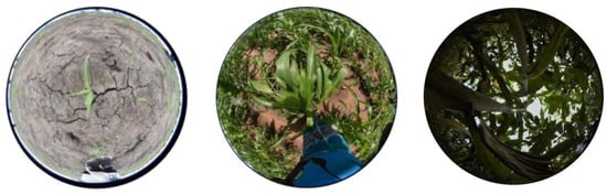
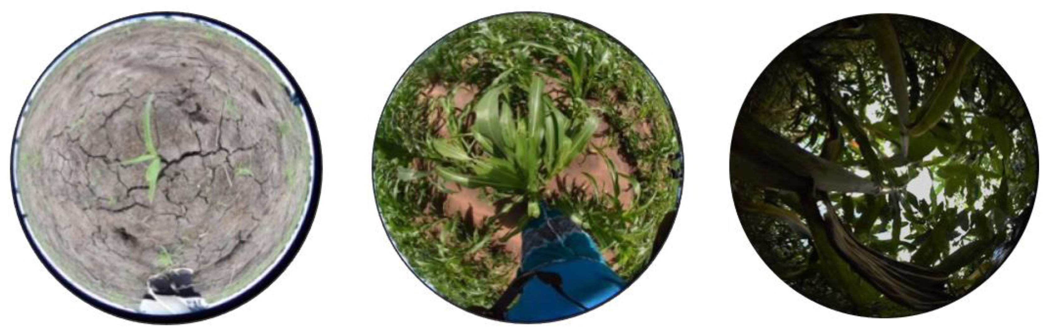
Figure 2.
Example DHP images of maize fields capturing different growth stages in the Phalombe district. Images were taken on the following dates (from left to right): 23 December 2019 (seeding), 11 January 2020 (vegetative), and 23 February 2020 (grain-filling) to capture maize main growth stages.
2.2.1. LAI Measurements
In situ LAI was used to evaluate the satellite-derived LAI (Section 2.4.2), which was further used to estimate crop yield. In situ LAI was assessed by using digital hemispherical photography (DHP), following the Committee on Earth Observation Satellites (CEOS) Working Group on Calibration and Validation (WGCV) Land Product Validation (LPV) protocol [41]. In each field, eight to thirteen DHP images were acquired by using a Nikon D5600 digital single-lens reflex (DSLR) camera and Sigma 4.5 mm F2.8 EX DC HSM fisheye lens. The images were taken with automatic exposure [42]. DHP images were collected in three phases (December 2019 to January 2020, February 2020, and March 2020) to capture key growth stages during the growing season (Figure 2). In the earlier growth stages, downward-facing images were obtained at the operator’s shoulder height, whilst upward-facing images were utilized in later phases, when the crop was taller than shoulder height. In total, approximately 2600 images were used for LAI retrieval. A 90° mask was applied to the downward-facing images to exclude the operator. All images were first classified and further processed to estimate LAI on the basis of gap fraction at 57.5° (±5°), as further detailed by Brown, et al. [43].
2.2.2. Biomass and Yield Measurements
Crop cutting measurements, considered to be the best standard of yield estimates [28], were used to measure maize biomass and yield in the sampled fields. For field sampling and yield measurements, the Food and Agriculture Organization (FAO) crop statistics protocol was followed, which suggests that at least three random subplots of 1 × 1 m are sampled within each field [44]. To increase the level of precision and considering that maize is generally spaced at a distance of approximately 75 cm in Southern Malawi, larger subplots of 1 × 2 m were sampled in this study, thus allowing us to harvest four to eight planting stations in each plot. Three of these subplots were established in each field to represent the whole field in terms of yield variation, and the mean value of the subplots was calculated to represent the whole field. The choice of the number and size of subplots was further guided by consulting local stakeholders and previous studies [9], whilst also considering trade-offs in terms of logistical practicability. In each subplot, the grain was shelled from the cob and then weighed, and grain moisture content was measured by using a grain moisture meter [45]—MC 7825G. Maize yield was adjusted to 12% moisture content based on fresh weight and moisture content [46]. In addition, aboveground maize biomass was measured by harvesting the maize canopy and weighing air-dried biomass. The ratio between yield and maize biomass was calculated to determine the harvest index, showing the proportion of the total aboveground biomass contributing to yield [47]. The harvest index was used to investigate its impact on yield model accuracy.
2.3. Official Yield Data and Maize Mask Dataset
Official crop yield data in 2020 were accessed through the Ministry of Agriculture in Malawi. The official yield data were available at the EPA level through the aggregation of plot-level yield measurements. For this study, maize yield data were retrieved for the three EPAs where the field plots were selected for in situ yield data collection. The official maize yield data were measured by following standard crop-cutting protocol in the field rather than relying on desk-based estimation, therefore providing a more reliable evaluation. The official maize-yield data were further used to test the feasibility of applying the EO-based model to a larger region than that over which it was calibrated. Application of the EO-based model was restricted to maize areas identified by using the malawi maize mask dataset (accessed through the World Bank Data Catalog), which was developed based on Sentinel-2 satellite imagery and complementary georeferenced plot-level data from national household surveys [48]. This dataset includes 10 m spatial resolution maize mask maps across Malawi for each rainy season during the period of 2016–2019. In this study, the maize crop mask for 2019 was used.
2.4. PlanetScope and Sentinel-2 Data
PlanetScope and Sentinel-2 satellite data were used to compare accuracy in yield estimation when using commercial high-spatial-resolution imagery over freely available imagery, while keeping in mind sensor differences and trade-offs between accuracy and cost when using these two datasets. The PlanetScope Level-3 Analytic Ortho Tile product with four spectral bands, namely blue, green, red, and near-infrared, was used. This product is both radiometrically and geometrically corrected. Cloud-free imagery during the growing season from November 2019 to April 2020 was selected (Table 1). The Sentinel-2 L2A surface reflectance data corrected using the Sen2Cor algorithm [49], were obtained and further analyzed in the Google Earth Engine platform [50]. Seven bands of visible, red-edge, and near-infrared covering the same phenological stage from November 2019 to April 2020 were used (Table 1). In addition, the clouds cirrus and shadow were masked out by using cloud mask bands.

Table 1.
Dates of the satellite data used during maize growing season, from November 2019 to April 2020, in the investigated test sites in Malawi.
2.4.1. Vegetation Indices (VIs)
VIs which proved capable of estimating crop yield in smallholder farming systems (Table 2) were investigated (Burke and Lobell 2017; Jain et al., 2019; Jin et al., 2017). In addition, red-edge VIs from Sentinel-2 images were calculated because of their good performance in estimating green LAI and chlorophyll content in maize fields [51,52,53,54,55]. The VIs were calculated at spatial resolutions of 3 m for PlanetScope imagery and 10 m for Sentinel-2 imagery (resampled 20 m red-edge bands to 10 m), respectively. Spatially, the field-averaged VI and LAI derived from satellite data (Section 2.4.2) were calculated. In addition, the standard deviation of VI and LAI values within each field was calculated to estimate within-field variation in terms of yield. The number of pixels falling inside each plot was calculated for each spatial resolution to understand the number of pixels required in order to capture within-field variation. Temporally, the maximum and median values, as well as mean values, were calculated across the growing season. This is necessary for maize yield estimation, as maize and intercrops appear in different growth stages. The accuracy of the temporal aggregation method in estimating maize yield was assessed. In addition, to further minimize the impact of cloud contamination and to avoid false positive values, a higher temporal resolution of VI and LAI values was constructed by using temporal interpolation [56], as this has been proven to improve empirical estimations of grain yield [57]. The discrete Fourier transform (DFT) [58,59] was used to interpolate between cloud-free Sentinel-2 VI and LAI values throughout the growing season on a per-pixel basis (Waldner et al., 2019). The selection of coefficients (i.e., phase of harmonic fits) was based on a study in East Africa and implemented in Google Earth Engine (Jin et al., 2019). Similarly, the seasonal mean, median, and maximum VIs/LAI were computed over interpolated data.
Table 2.
Vegetation indices (VIs) and bands from Sentinel-2 and PlanetScope used for crop yield estimation.
2.4.2. LAI Retrieval
In addition to the LAI measurements from the DHP images, the LAI was also retrieved by using the radiative transfer model-based Simplified Level 2 Product Prototype Processor (SL2P) algorithm [69]. The SL2P algorithm was developed to systematically retrieve vegetation biophysical variables from Sentinel-2 Multispectral Instrument (MSI) data and is executed in the Sentinel Application Platform (SNAP). SL2P retrievals are sensitive to the ‘effective LAI’ [70], which was compared with in situ ‘effective LAI’. For correlating in situ LAI to Sentinel-2 derived LAI, the Sentinel-2 images closest to the DHP acquisition dates were chosen, where the average acquisition date difference for two measurements was less than three days.
2.5. Model Development and Performance Evaluation
2.5.1. Linear Regression Model and Its Accuracy Assessment
Empirical linear regression models between the field-measured yields and VIs/LAI computed from Sentinel-2 and PlanetScope data were developed to estimate maize yield. To assess the model performance, the coefficient of determination (R2), p-value, root mean square error (RMSE), and normalized root mean square error RMSE (nRMSE: RMSE divided by observed yield difference) were calculated. In addition, standard deviations of R2 and RMSE were calculated from 10-fold cross-validation with 500 repeats. The models with the highest estimation accuracy (i.e., the highest R2 and lowest RMSE) were applied to estimate maize yield for the whole area of the three EPAs (Figure 1) and validated against official maize yield statistics. To avoid the extrapolation of the empirical models, yield estimation was restricted to maize areas where Vis/LAI satellite estimates fell within the range of the training data.
2.5.2. Evaluating Factors Influencing Model Performance
Model residuals were plotted against the factors (field size, within-field variation, intercropping practices, and the harvest index (described in Section 2.2.2) to understand if and how these factors influence yield estimation accuracy. To evaluate how the spatial resolution of satellite data affects yield estimation accuracy, after validating the EO data at their native spatial resolution, i.e., 3 m for PlanetScope and 10 and 20 m for Sentinel-2 data, PlanetScope data were aggregated to coarser spatial resolutions (from 10 to 100 m, at 10 m intervals; and, afterward, at 100 m intervals up to 500 m) to assess how the model accuracy is affected by the EO spatial resolution, whilst removing the impact of differences introduced by the use of different sensors. As the PlanetScope data were resampled to lower spatial resolutions, fields that accounted for less than half a pixel (after the resampling) were not considered. This resulted in approximately 16 small fields being excluded from the analysis when resampling to resolutions coarser than 350 m. An overview of the data and the methodology is presented in Figure 3.
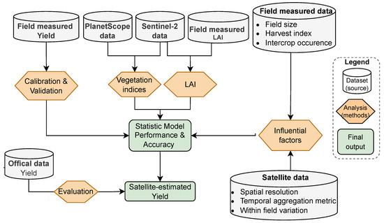
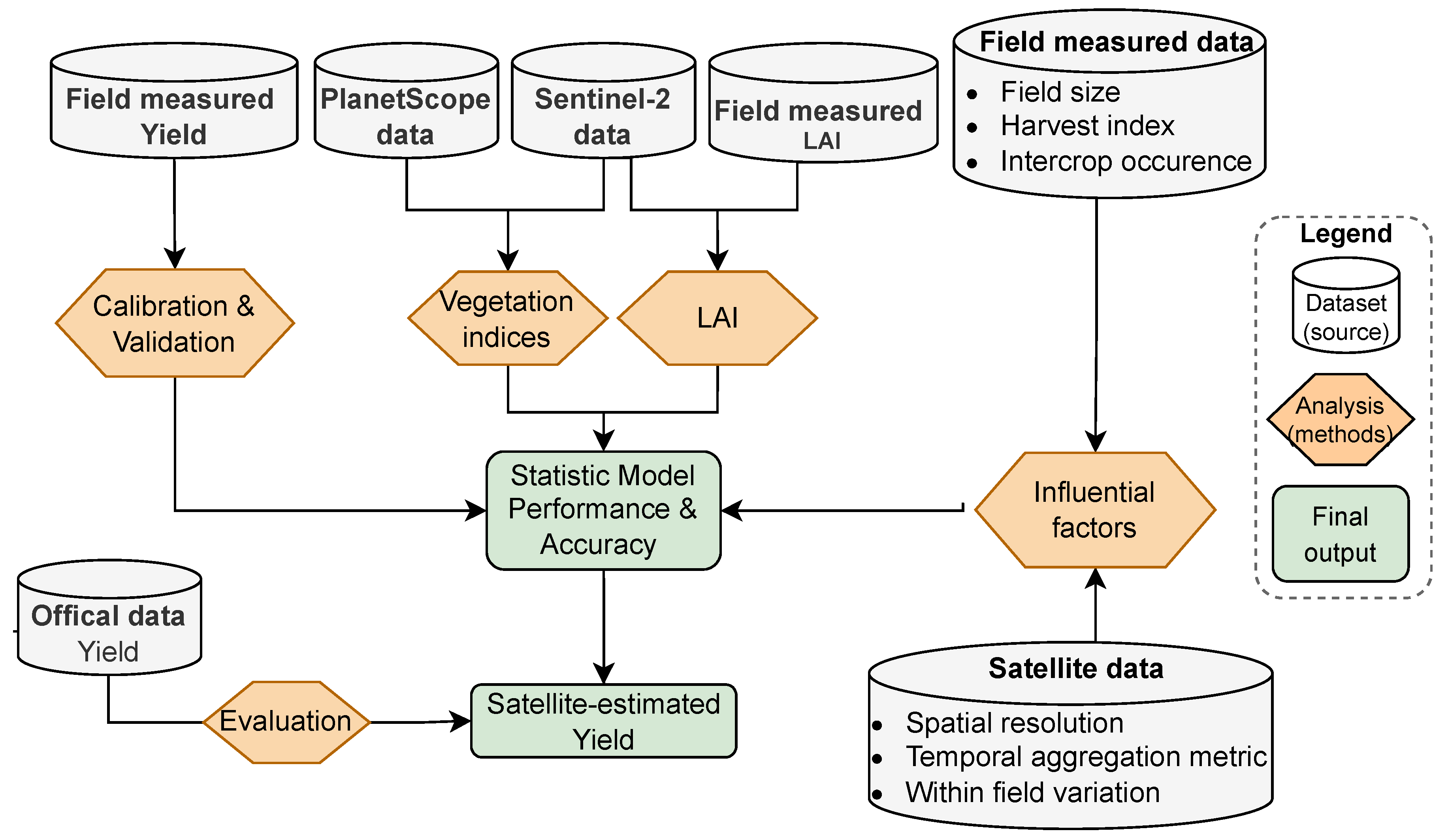
Figure 3.
Flowchart showing the approach used to estimate crop yield and evaluate factors influencing model accuracy.
3. Results
3.1. Field Characteristics and Intercropping Practices
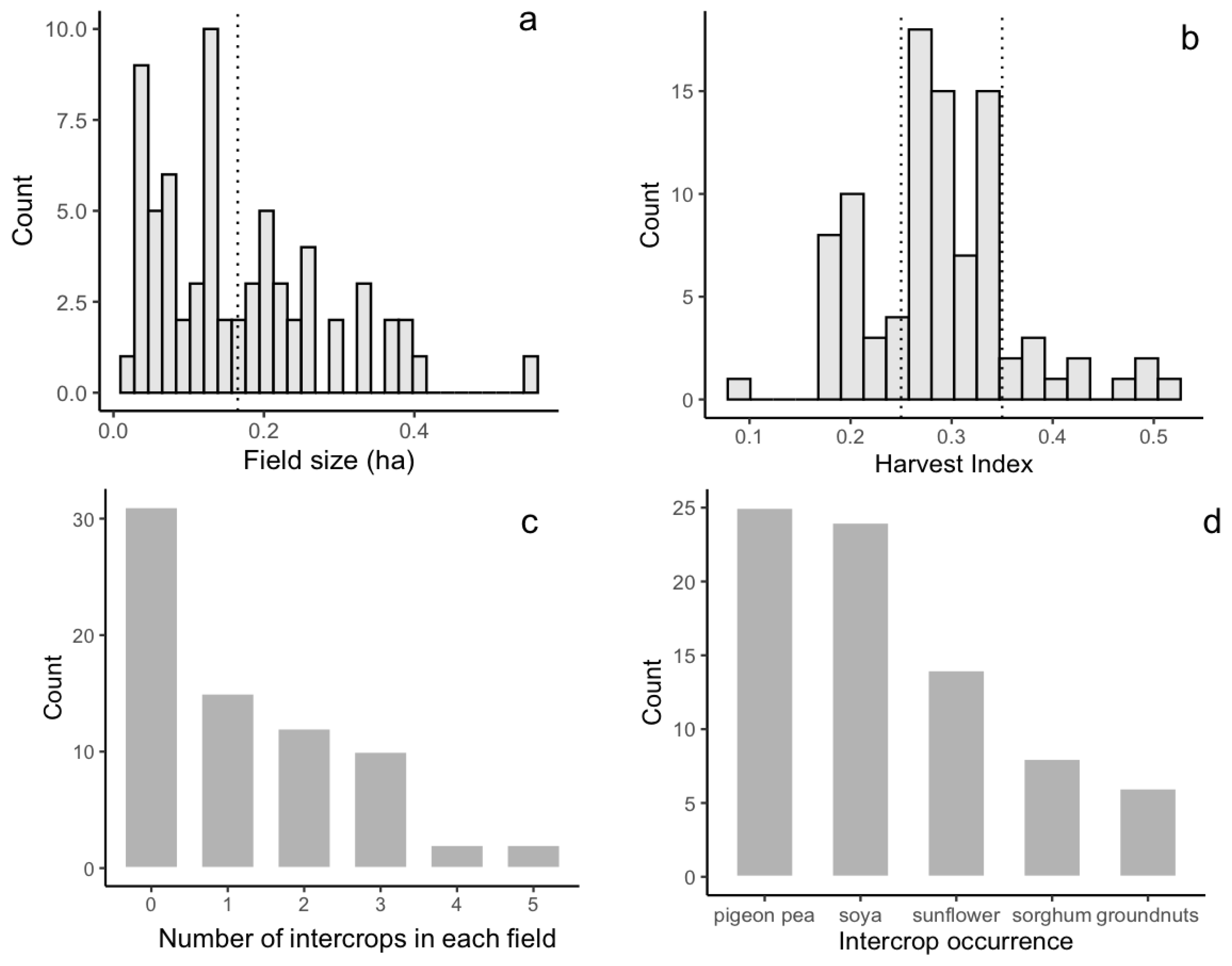
The investigated field size ranges from 0.03 to 0.55 ha, with a mean value of 0.17 ha (Figure 4a). The number of Sentinel-2 pixels (at 10 m resolution) falling inside of the maize plots varied from 3 to 58, with an average of 17 pixels. The number of PlanetScope pixels (at 3 m resolution), instead, varied between 35 and 640, with an average value of 191 pixels. The harvest index showed high variability in the investigated fields, ranging from 0.18 to 0.55 (Figure 4b). Intercropping was practiced at half of the investigated fields: 18% of the investigated fields were cultivated with one intercrop, whilst nearly 33% were cultivated with two intercrops other than maize. Some fields were cultivated with up to four different intercrops (Figure 4c). Relay intercropping is the most common practice: intercrops were planted when maize had grown to a certain height, and they reached maturity only after the maize was harvested. This practice led to dominant maize foliage on the top of the canopy during the peak of the growing season that was slowly taken over by the lower intercrops during maize senescence. Intercropping was practiced with varying crop types and densities among the fields, with soybean and pigeon pea being the most common, followed by sunflower and sorghum (Figure 4d).

Figure 4.
Maize field characteristics among 150 investigated fields. (a) Histogram of field size. The dotted line shows the mean field size. (b) Histogram of harvest index. Dotted lines show the 25th (0.25) and 75th percentiles (0.35) of the harvest index, which were used to group the harvest index into low, middle, and high categories. (c). Histogram of number of intercrops planted in maize fields. (d) Histogram of intercrop types in maize field.
3.2. Crop Yield Estimation Using VIs and LAI with Different Spatial Resolution
When comparing model accuracy with different temporal aggregation methods (seasonal maximum, median, and mean VI), the models based on the maximum VI values demonstrated the highest accuracy for all investigated VIs (Supplementary Tables S1 and S2). This was the case for both PlanetScope and Sentinel-2 data. Meanwhile, there was no substantial improvement when using temporally interpolated VIs compared to original values (Supplementary Table S1). Similar to the VIs, the maximum LAI calculated from both the original and interpolated values demonstrated better estimation accuracy than the mean and median LAI (Supplementary Table S3). As with the VI results, the temporally interpolated LAI did not demonstrate any improvements compared to the original LAI values (including the mean, median, and maximum) (Supplementary Table S3). As such, models calibrated using seasonal maximum VIs/LAI are presented hereafter.
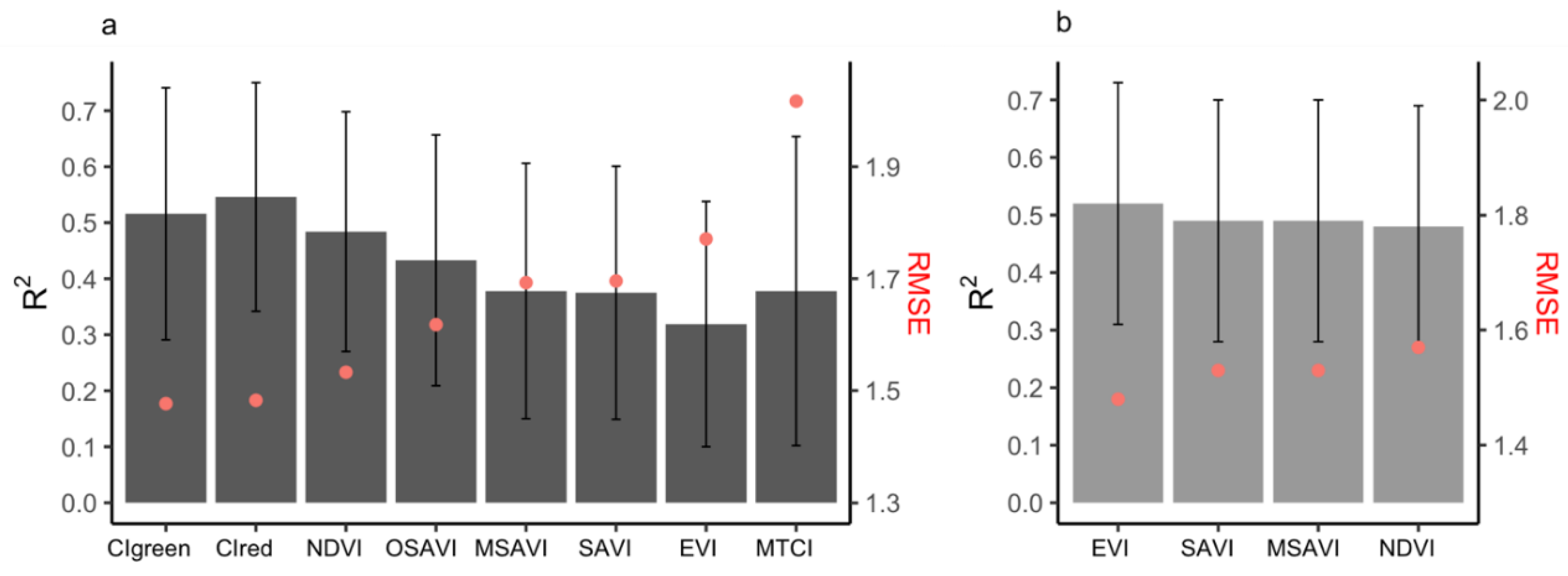
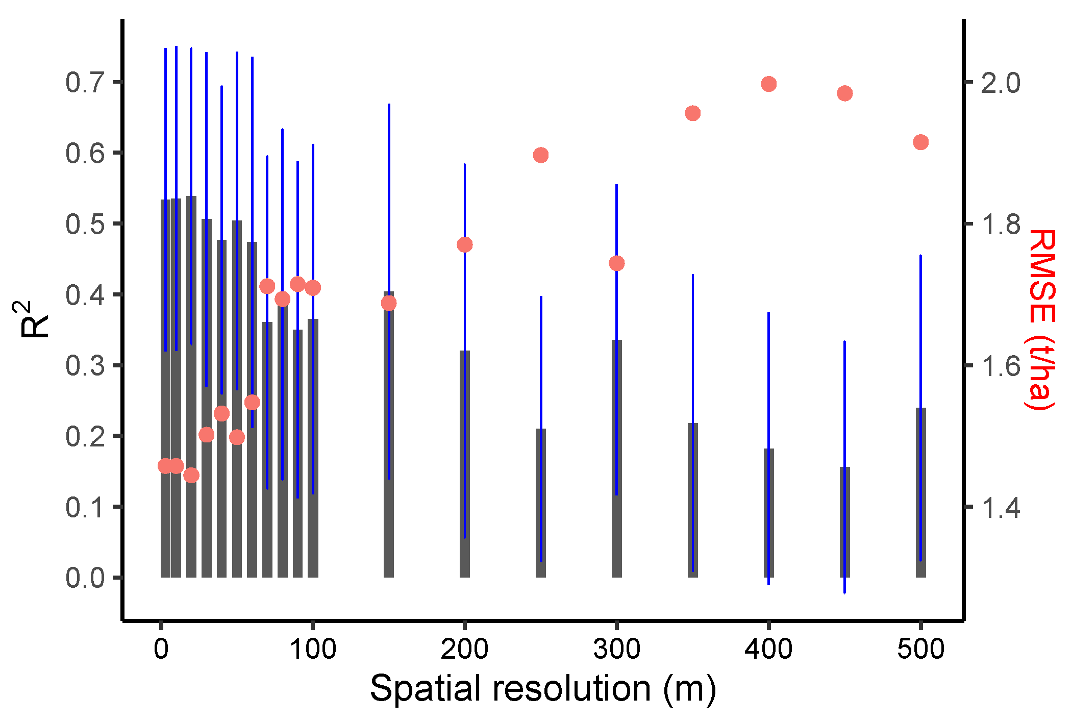
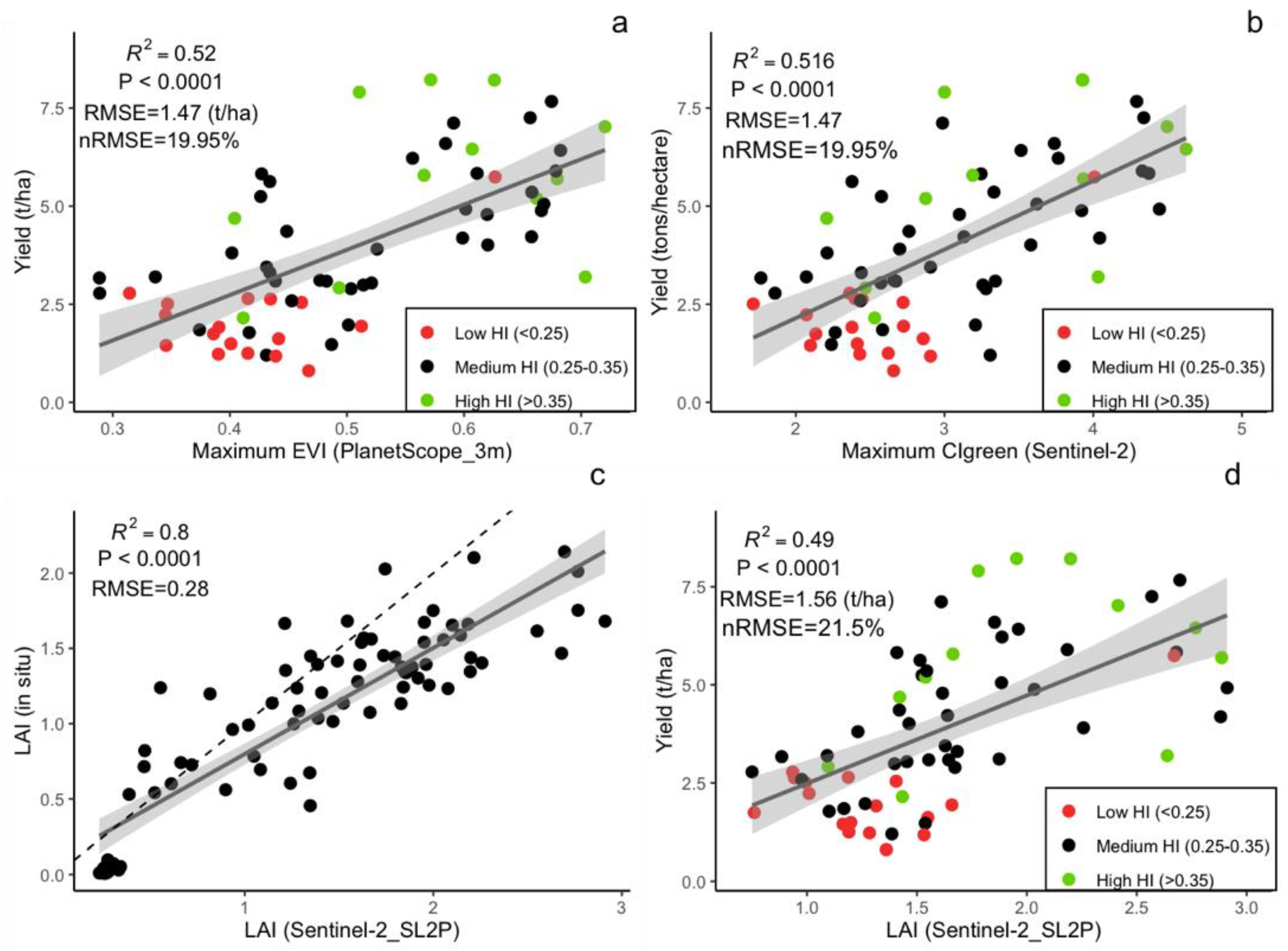
When comparing different spatial resolutions, models that were calibrated using the PlanetScope EVI (which achieved higher accuracy compared to other Vis; see Figure 5b and Supplementary Table S2) were developed for spatial resolutions of 3 to 500 m (Figure 6). The results demonstrated that crop-yield estimation accuracy was relatively stable at spatial resolutions finer than 20 m (i.e., 3 and 10 m) (Figure 6). However, at spatial resolutions coarser than 20 m, the model accuracy reduced sharply, with further decreases in spatial resolution (Figure 6). In addition, when the predictive power of the two satellite datasets (Sentinel-2 and PlanetScope) with different spatial resolutions was compared, we found that the model with the highest accuracy that was calibrated by using 3 m PlanetScope data (EVI, R2 = 0.52, nRMSE = 19.95%) only demonstrated a marginal improvement over 10 m Sentinel-2 data (CIgreen, R2 = 0.51, nRMSE = 19.95%) (Figure 5a,b and Figure 7a,b). Specifically, models based on red-edge indices (CIgreen and CIred) estimated the maize yield with the highest accuracy when using the Sentinel-2 data (Figure 5a and Supplementary Table S1). The model based on the EVI calculated from PlanetScope showed a slightly higher accuracy (R2 = 0.52, nRMSE = 19.95%) when compared to other VIs computed from the same dataset (Figure 5b and Supplementary Table S2) and a significantly higher accuracy than the EVI computed from Sentinel-2 (R2 = 0.32, nRMSE = 23.8%) (Supplementary Tables S1 and S2; Figure 5a,b). When estimating maize yield by using the LAI, the Sentinel-2 LAI was firstly evaluated with respect to in situ LAI (Figure 7c). The Sentinel-2 LAI demonstrated a strong linear correlation (R2 = 0.8, RMSE = 0.28) but presented an overestimation of the in situ LAI for high LAI values, i.e., during the late growing season (Figure 7c). The model calibrated using Sentinel-2 LAI had lower accuracy in estimating yield (average R2 = 0.49, nRMSE = 21.5%) compared to CIgreen from Sentinel-2 (i.e., R2 = 0.52, nRMSE = 19.95%) (Figure 7a,d). Therefore, the model calibrated using Sentinel-2 CIgreen was used for further analysis.
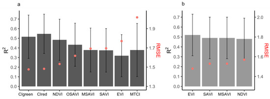
Figure 5.
The accuracy (R2 and RMSE) of the empirical models using the seasonal maximum VIs listed in Table 2, using (a) Sentinel-2 seasonal maximum VIs (only top eight shown) at spatial resolution of 10 m and (b) PlanetScope seasonal maximum VIs at spatial resolution of 3 m. Error bars indicate the standard deviation of R2 assessed from the 10-fold cross-validation realizations, whilst the red dots refer to the RMSE (t/ha).

Figure 6.
Performance of linear regressions between in situ yield and PlanetScope EVI resampled to different spatial resolutions (3, 10 m, 20 m, …, 100 m, 200 m, …, 500 m). Gray bars indicate R2, and the blue lines indicate R2 standard deviation. The red dots show RMSE (right-hand y-axis).

Figure 7.
Linear correlation between in situ maize yield from 68 fields and (a) maximum PlanetScope EVI and (b) maximum CIgreen; (c) Correlation between in-situ LAI and SL2P-derived LAI; (d) linear regression between in situ yield and seasonal maximum SL2P-derived LAI. The colored dots indicate the harvest index (HI) category.
3.3. Factors Influencing Model Accuracy
The evaluation of intercropping practices, field size, within-field variability, and harvest index against model residuals showed the mixed results. The intercropping practice reduced model accuracy, as the mean model residuals are lower in fields cultivated with pure maize fields (1 t/ha) compared to intercropped fields (1.3 t/ha) (Figure 8a). In addition, the harvest index was positively correlated to the model residuals (observed yield minus estimated yield) that were calibrated using Sentinel-2 CIgreen, demonstrating that the linear models tended to overestimate (/underestimate) yield for fields with a low (high) harvest index (Figure 7a and Figure 8b). No clear correlation pattern was observed when considering the correlation between model residuals and the field size (Figure 8c). Finally, model residuals were not correlated to within-field variation (Figure 8d).
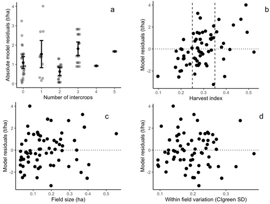
Figure 8.
Scatterplots between model residuals (observed yield minus estimated yield) and field characteristics: (a) number of intercrops in maize fields; (b) maize harvest index (the vertical dashed lines show the 25th (HI = 0.25) and 75th percentiles (HI = 0.35) of the harvest index); (c) maize field size; and (d) within-field variation defined as the standard deviation of CIgreen index. The horizontal dashed lines in each panel show residuals equal to zero.
3.4. Validation of the Models over a Larger Region Using Official Statistics
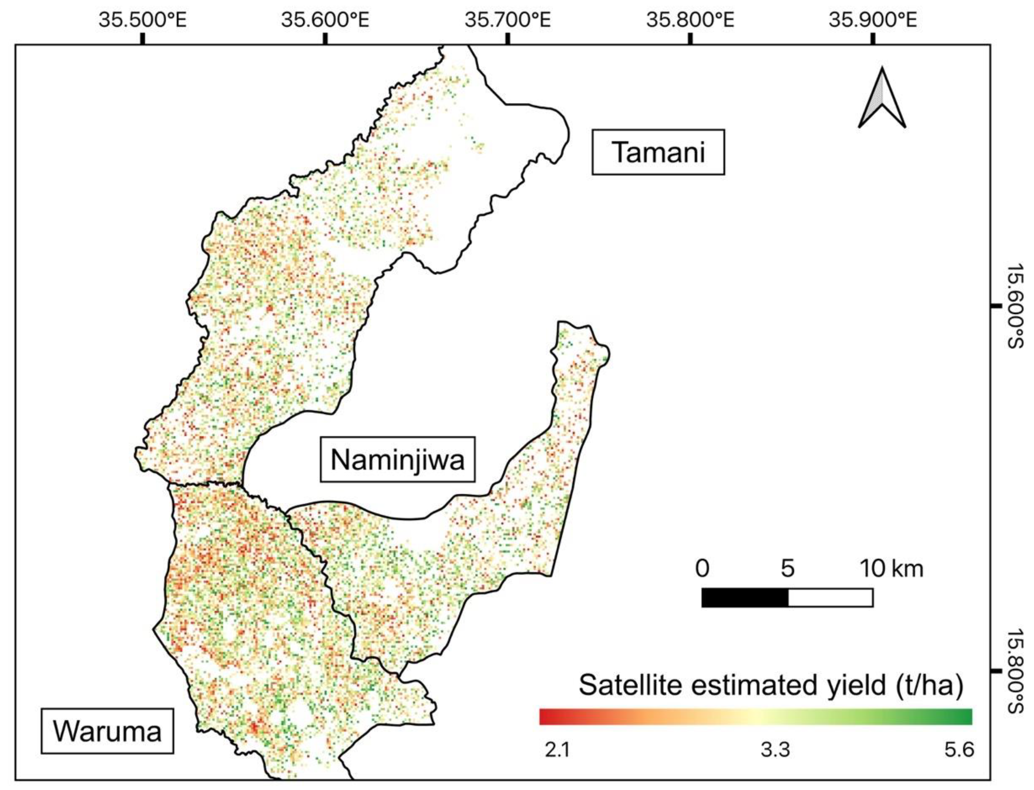
Our comparison between EO-estimated and official yield shows that EO estimates could capture the spatial variability of yield (Figure 9) that varied from 2.1 to 5.6 t/ha. The highest maize yield was found in the Naminjiwa EPA, while the lowest yield was found in the Tamani EPA (Table 3), both from EO estimates and the official estimates (Table 3). In absolute terms, however, EO-estimated yield tended to be higher, with average overestimation of 0.98 t/ha compared to official data (Table 3). In addition, bigger disparities existed for EPAs outside of the calibration region in the Lake Chilwa-Phalombe plain (Supplementary Figure S1), where EO-estimated yields were much higher than official estimates.
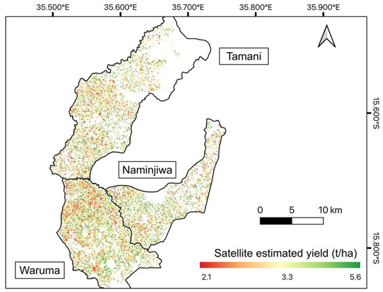
Figure 9.
Yield estimates for maize fields using the linear model with the highest accuracy developed from the Sentinel-2 CIgreen index (Figure 7b). White areas represent non-maize fields.
Table 3.
Comparison between satellite data estimated maize yield by using red-edge VIs at spatial resolution of 10 m (R2 = 0.52, nRMSE = 19.95%) and official maize yield estimates at the EPA administrative level.
4. Discussion
This study examines to what extent EO data can estimate maize yield for smallholder intercropped fields in order to provide a better understanding of yield estimation when utilizing such dataset for operational purposes. By evaluating factors including temporal and spatial resolution of satellite data, field size, within-field variability, harvest index and the occurrence of intercrops that affect yield estimation accuracy, our study identified the challenges and opportunities for estimating yield by using EO data in smallholder intercropped fields, whilst adding to the limited amount of the literature that estimates crop yield in smallholder farms in SSA.
4.1. Performance of Optical EO Data in Estimating Yield in Intercropping Fields
Considering that optical satellite data showed a high cloud-cover percentage during the rainy (and maize growing) season in Malawi, we constructed a higher temporal resolution of VIs/LAI and evaluated how temporal resolution and temporally aggregated values (e.g., mean, maximum, and median value) affect yield estimation accuracy. Our results revealed that there was no substantial improvement when using temporally interpolated VIs/LAI compared to original values (Supplementary Tables S1–S3), indicating that temporal interpolation methods are unlikely to improve yield estimation accuracy. Indeed, previous studies have found that simple metrics remain the best choice when satellite data are sparse, while advanced smoothing methods based on phenological profiles are recommended when temporal resolution is ≤5 days (Waldner et al., 2019). We found that the peak value of all VIs and LAI both from original and temporarily interpolated values provided a better yield estimation accuracy than mean/median values (Supplementary Tables S1 and S2). Similar results have also been shown by other studies (Zhao et al., 2020), suggesting that the peak value best captures photosynthetic activity and, therefore, serves as a good predictor for yield estimation. In our study area, the dates when crops reach peak greenness range from the end of January to the middle of March. These dates can be related to crop physiology, seed varieties, growing degree days (temperature), or management practices, but they can also be impacted by satellite data availability during the growing season. Therefore, obtaining more frequent imagery during the peak of the growing season would be useful for improving yield predictions.
The lack of in situ yield data is another difficulty in estimating yield in intercropped smallholder fields in SSA. Although 68 fields were sampled in Southern Malawi—a number that is not sufficient enough to upscale our findings to the national scale—this sample size was considered to be reasonable in the African setting for stable model performance (Burke et al., 2021). Our study indicates that models calibrated with in situ data provide a better estimation accuracy (i.e., R2 = 0.51) than models trained with farmer self-reported data and official data (i.e., R2 = 0.1–0.4), as shown by previous studies (Burke et al., 2021; Burke and Lobell 2017). This stresses the importance of collecting ground data in SSA where the paucity of ground data is the largest constraint to satellite-based model performance [8]. Collectively collecting ground data on crop and field characteristics, as well as sharing and making the dataset publicly available, would advance the field of yield monitoring and modeling using satellite imagery.
This study provides insights on which optical satellite inputs of VIs and LAI could serve for the operational purpose of rapid and large-scale yield assessment in Southern Malawi. As seasonal maximum VIs/LAI was the best predictor of maize yield, it follows that Sentinel-2 data could forecast maize yield 1–2 months in advance of harvest with moderate accuracy (R2 = 0.51, nRMSE = 19.95%). However, this assessment pertains to the areas where the model was calibrated with ground data (Figure 9). Indeed, the model prediction uncertainties tend to be larger when applying the models outside the calibration area (Supplementary Figure S1). As such, model calibration using in situ data is necessary for the operational purposes of yield monitoring. In addition, further analysis is needed to test whether the model accuracy still holds outside of the calibration season of 2019/2020. Finally, although VIs or LAI for empirical yield estimation have been widely adopted in previous studies [15,16,17], this and previous studies in Kenya and Mali have found that VIs can explain maize and cotton yield variation with an R2 ranging from 0.3 to 0.6 (Burke and Lobell 2017; Jin et al., 2017; Lambert et al., 2018). Indeed, using mainly satellite inputs of VIs or LAI and empirical models carries limited accuracy and may not capture the full variation of actual yield, as spectral properties (as captured by VIs) reflect photosynthetically active biomass within fields, including maize, weeds, and intercrops, which is only indirectly related to crop maize yield [71]; however, maize foliage is dominant over other intercrop foliage, as demonstrated by field photos (Supplementary Figure S2). In this case, integrating information on environmental conditions could potentially improve yield estimation accuracy.
4.2. Impact of EO Spatial Resolution on Yield Estimation Accuracy
Although PlanetScope data could capture 191 pixels (at 3 m resolution)—that is 10 times more than using Sentinel-2 data (17 pixels at 10 m resolution)—our study and others have reported limited improvements when using finer spatial resolution satellite data (i.e., 3 m) compared to the spatial resolution of 10 m (i.e., Sentinel-2). For example, for sorghum yield, Lobell, et al. [72] found similar accuracy by using both 3 and 30 m data in smallholder fields in SSA, suggesting that the benefits of using a finer spatial resolution (e.g., <10 m) for yield estimation at the field scale might not be substantial. Given that model residuals in our study were relatively consistent irrespective of field size and within-field variation, and yield estimation accuracy dropped when spatial resolution is coarser than 20 m, while it stays stable when finer than 10 m, this might suggest that satellite data with a 10 m spatial resolution offer a cost-effective choice for yield estimation in smallholder fields in Southern Malawi. However, the optimal spatial resolution may depend on the field size and heterogeneity of landscape, in addition to the scale of yield estimation (field, local or regional) and requirements of accuracy by stakeholders (i.e., farmers, crop insurers, or officials). Therefore, the proposed optimal resolution and number of pixels for smallholder farming yield estimation need to be tested in different sites and crop types. Trade-offs between accuracy and cost should also be considered when using high-resolution satellite data (i.e., finer than 3 m). UAV data that were widely used for precision soil monitoring and yield prediction [73,74] could provide a link between field and satellite observation for better monitoring field variation. Finally, spectral resolution is also critical for yield estimation when using satellite data. Comparing model accuracy when using Sentinel-2 (10 m) and PlanetScope data (3 m), our study demonstrates the importance of red edge-based VIs (CIred and CIgreen) from Sentinel-2 in yield estimation, as spectral reflectance in the red edge has a strong linear correlation with canopy chlorophyll content [68,75]. Therefore, models utilizing the red edge part of the electromagnetic spectrum have a higher ability to predict crop yield, as also shown by other studies [72,76].
The positive correlation between the harvest index and residuals indicates that including the harvest index could improve model accuracy. The wide range of harvest index values (i.e., from 0.18 to 0.55) found in this study indicates varying environmental conditions (e.g., water or nutrient deficits) [47], particularly during the crop reproductive stage. Stress factors such as extreme temperatures and limited water availability may cause strong decreases in harvest index and, therefore, yield [47]. As such, including environmental variables such as soil moisture and climate information [32,77] during the reproductive stage may also be beneficial for yield estimation accuracy. As the correlation between biomass and final yield can be non-linear, integrating environmental variables and applying a non-linear model could offer further improvements in yield estimation accuracy [77]. In this case, synergizing multiple satellite data sources, including thermal and microwave data that reflect soil moisture, could be further explored for yield estimation [78].
4.3. Future Research Paths for Understanding Intercropping Practice and Better Estimating Yield
Intercropping has been widely practiced in Africa for a long time [79]; however, intercropping practices have rarely been identified when estimating yield in previous EO-based studies [7,10,18]. This study found that intercropping practices reduce model accuracy and suggests that the potential impact of intercropping on maize yield estimation might be minimized when using seasonal maximum VIs/LAI values. Often, as intercrops are planted and harvested after maize, intercrops usually grow underneath the maize canopy during the peak of the growing season. An illustration from field photographs (Supplementary Figure S2) shows that green intercrops appear at the senescent stage of the maize crops, resulting in relatively higher mean greenness than maize alone across the growing season. Therefore, the seasonal mean value of satellite VIs/LAI calculated from intercropped fields is more likely to include the signal from the intercrops, whilst the peak value from satellite VIs/LAI is likely to capture the fully developed maize canopy, with understory intercrops contributing less to the satellite signal. In our study, we found that peak values showed, indeed, better prediction accuracy compared to mean values. As such, this result suggests that seasonal maximum VIs/LAI values might reduce the potential impact of intercropping on maize yield estimation. However, further studies are needed to test the above arguments. One option would be to compare the time series of vegetation greenness of pure maize fields and intercropped maize fields by using fine temporal resolution satellite data (e.g., <5 days). In addition, examining field greenness after maize harvesting by using sufficient satellite observations could also be used to identify the presence/absence and intensity of intercropping. This is critical to more accurately estimate yield, including main maize, as well as intercrops, while the only estimation of maize yield resulted in the underestimation of total yield. Therefore, the practices of intercropping and its impacts on total yield need further investigation for better estimating food production.
5. Conclusions
This study investigated the performance of EO data for estimating maize yield in intercropped fields through field investigations and multisource satellite data. For this, comprehensive field data (i.e., field size, yield, the presence and type of intercrops, harvest index, and LAI) were collected in Southern Malawi to calibrate EO-derived VIs and LAI. The results showed that, despite mixed pixels in the EO data from maize and intercrops, moderate accuracy (R2 = 0.51, nRMSE = 19.95%) was achieved by using the red-edge band VI. Having evaluated the impact of spatial resolution on yield estimation accuracy, this study concluded that high-resolution data (e.g., PlanetScope 3 m) provide only marginal improvements in yield estimation accuracy. Our findings suggest that Sentinel-2 data offer the potential for operational monitoring of maize yield in intercropped smallholder fields in Southern Malawi. The presence of intercrops complicates yield estimation using EO data, but our results indicate that the use of the seasonal maximum VI value could lessen the impact of intercrop presence. However, difficulties in measuring and estimating intercrop yield need to be overcome in order to accurately measure total yield, which is critical for understanding and closing the yield gap in SSA.
Supplementary Materials
The following supporting information can be downloaded at: https://www.mdpi.com/article/10.3390/rs14102458/s1, Figure S1: Comparison between official yield and satellite data estimated yield; Figure S2: Field photos showing maize-legume intercropped plots at peak growing season and harvesting stage; Table S1: Accuracy assessment (R2 and RMSE) of linear regression models between Sentinel-2 VIs and yield; Table S2: Accuracy assessment (R2 and RMSE) of linear regression models between PlanetScope VIs and yield; Table S3: Accuracy assessment (R2 and RMSE) of linear regression models between Sentinel-2 retrieved LAI and yield.
Author Contributions
Conceptualization, C.L., J.D.; Methodology, C.L., E.G.C., O.K., L.A.B., T.P.C. and C.N.; Validation, C.L., J.D.; Formal Analysis, C.L.; Investigation, C.L., E.G.C. and O.K.; Data Curation, C.L., E.G.C. and O.K.; Writing—Original Draft Preparation, C.L.; Writing—Review & Editing, C.L., J.D., L.A.B., D.A., C.N., Y.L. and J.S.; Visualization, C.L.; Supervision, J.D.; Project Administration, J.D., J.S.; Funding Acquisition, J.S. All authors have read and agreed to the published version of the manuscript.
Funding
This work and APC was funded through the ‘Building REsearch Capacity for sustainable water and food security In drylands of sub-saharan Africa’ (BRECcIA) which is supported by UK Research and Innovation as part of the Global Challenges Research Fund, grant number NE/P021093/1.
Data Availability Statement
Satellite imagery Sentinel-2 were accessed and processed through the Google Earth Engine platform (https://developers.google.com/earth-engine/datasets/catalog, accessed on 18 July 2020), the PlanetScope satellite data were accessed through the ESA third party data access programme. Official yield data was provided by Ministry of Agriculture, Planning Department of Malawi. Official yield data and field data on maize plots coordinates, maize yield, LAI and etc is available upon reasonable request from the authors.
Acknowledgments
Special thanks to the Ministry of Agriculture, Planning Department of Malawi for providing the agricultural production estimate data used in this study. We are thankful to European Space Agency’s Third Party Missions programme for providing Planetscope data for the project (Project ID: 59585).
Conflicts of Interest
The authors declare no conflict of interest.
References
- Fischer, R.A.; Connor, D.J. Issues for cropping and agricultural science in the next 20 years. Field Crops Res. 2018, 222, 121–142. [Google Scholar] [CrossRef]
- Barbier, E.B.; Hochard, J.P. Land degradation and poverty. Nat. Sustain. 2018, 1, 623–631. [Google Scholar] [CrossRef]
- Savary, S.; Willocquet, L.; Pethybridge, S.J.; Esker, P.; McRoberts, N.; Nelson, A. The global burden of pathogens and pests on major food crops. Nat. Ecol. Evol. 2019, 3, 430–439. [Google Scholar] [CrossRef] [PubMed]
- Agutu, N.O.; Awange, J.L.; Zerihun, A.; Ndehedehe, C.E.; Kuhn, M.; Fukuda, Y. Assessing multi-satellite remote sensing, reanalysis, and land surface models’ products in characterizing agricultural drought in East Africa. Remote Sens. Environ. 2017, 194, 287–302. [Google Scholar] [CrossRef] [Green Version]
- Chakraborty, S.; Newton, A.C. Climate change, plant diseases and food security: An overview. Plant Pathol. 2011, 60, 2–14. [Google Scholar] [CrossRef]
- Huang, J.; Gómez-Dans, J.L.; Huang, H.; Ma, H.; Wu, Q.; Lewis, P.E.; Liang, S.; Chen, Z.; Xue, J.-H.; Wu, Y.; et al. Assimilation of remote sensing into crop growth models: Current status and perspectives. Agric. For. Meteorol. 2019, 276-277, 107609. [Google Scholar] [CrossRef]
- Burke, M.; Lobell, D.B. Satellite-based assessment of yield variation and its determinants in smallholder African systems. Proc. Natl. Acad. Sci. USA 2017, 114, 2189–2194. [Google Scholar] [CrossRef] [Green Version]
- Burke, M.; Driscoll, A.; Lobell, D.B.; Ermon, S. Using satellite imagery to understand and promote sustainable development. Science 2021, 371, eabe8628. [Google Scholar] [CrossRef]
- Jain, M.; Balwinder, S.; Rao, P.; Srivastava, A.K.; Poonia, S.; Blesh, J.; Azzari, G.; McDonald, A.J.; Lobell, D.B. The impact of agricultural interventions can be doubled by using satellite data. Nat. Sustain. 2019, 2, 931–934. [Google Scholar] [CrossRef]
- Lambert, M.-J.; Traoré, P.C.S.; Blaes, X.; Baret, P.; Defourny, P. Estimating smallholder crops production at village level from Sentinel-2 time series in Mali’s cotton belt. Remote Sens. Environ. 2018, 216, 647–657. [Google Scholar] [CrossRef]
- Funk, C.; Budde, M.E. Phenologically-tuned MODIS NDVI-based production anomaly estimates for Zimbabwe. Remote Sens. Environ. 2009, 113, 115–125. [Google Scholar] [CrossRef]
- Lobell, D.B. The use of satellite data for crop yield gap analysis. Field Crops Res. 2013, 143, 56–64. [Google Scholar] [CrossRef] [Green Version]
- Qader, S.H.; Dash, J.; Atkinson, P.M. Forecasting wheat and barley crop production in arid and semi-arid regions using remotely sensed primary productivity and crop phenology: A case study in Iraq. Sci. Total Environ. 2018, 613-614, 250–262. [Google Scholar] [CrossRef] [PubMed] [Green Version]
- Weiss, M.; Jacob, F.; Duveiller, G. Remote sensing for agricultural applications: A meta-review. Remote Sens. Environ. 2020, 236, 111402. [Google Scholar] [CrossRef]
- Leroux, L.; Castets, M.; Baron, C.; Escorihuela, M.-J.; Bégué, A.; Lo Seen, D. Maize yield estimation in West Africa from crop process-induced combinations of multi-domain remote sensing indices. Eur. J. Agron. 2019, 108, 11–26. [Google Scholar] [CrossRef]
- Johnson, M.D.; Hsieh, W.W.; Cannon, A.J.; Davidson, A.; Bédard, F. Crop yield forecasting on the Canadian Prairies by remotely sensed vegetation indices and machine learning methods. Agric. For. Meteorol. 2016, 218–219, 74–84. [Google Scholar] [CrossRef]
- Bolton, D.K.; Friedl, M.A. Forecasting crop yield using remotely sensed vegetation indices and crop phenology metrics. Agric. For. Meteorol. 2013, 173, 74–84. [Google Scholar] [CrossRef]
- Jin, Z.; Azzari, G.; Burke, M.; Aston, S.; Lobell, D.B. Mapping Smallholder Yield Heterogeneity at Multiple Scales in Eastern Africa. Remote Sens. 2017, 9, 931. [Google Scholar] [CrossRef] [Green Version]
- Leroux, L.; Baron, C.; Zoungrana, B.; Traoré, S.B.; Seen, D.L.; Bégué, A. Crop Monitoring Using Vegetation and Thermal Indices for Yield Estimates: Case Study of a Rainfed Cereal in Semi-Arid West Africa. IEEE J. Sel. Top. Appl. Earth Obs. Remote Sens. 2016, 9, 347–362. [Google Scholar] [CrossRef] [Green Version]
- Diouf, A.A.; Brandt, M.; Verger, A.; Jarroudi, M.E.; Djaby, B.; Fensholt, R.; Ndione, J.A.; Tychon, B. Fodder Biomass Monitoring in Sahelian Rangelands Using Phenological Metrics from FAPAR Time Series. Remote Sens. 2015, 7, 9122–9148. [Google Scholar] [CrossRef] [Green Version]
- Bégué, A.; Leroux, L.; Soumaré, M.; Faure, J.-F.; Diouf, A.A.; Augusseau, X.; Touré, L.; Tonneau, J.-P. Remote Sensing Products and Services in Support of Agricultural Public Policies in Africa: Overview and Challenges. Front. Sustain. Food Syst. 2020, 4, 58. [Google Scholar] [CrossRef]
- Inbal, B.-R.; Christina, J.; Brian, B.; Michael, H.; Felix, R.; Rogerio, B.; Mario, Z.; Mike, B.; Tamuka, M.; Chris, S.; et al. Strengthening agricultural decisions in countries at risk of food insecurity: The GEOGLAM Crop Monitor for Early Warning. Remote Sens. Environ. 2020, 237, 111553. [Google Scholar] [CrossRef]
- Fritz, S.; See, L.; Bayas, J.C.L.; Waldner, F.; Jacques, D.; Becker-Reshef, I.; Whitcraft, A.; Baruth, B.; Bonifacio, R.; Crutchfield, J.; et al. A comparison of global agricultural monitoring systems and current gaps. Agric. Syst. 2019, 168, 258–272. [Google Scholar] [CrossRef]
- Seguini, L.; Bussay, A.; Baruth, B. From extreme weather to impacts: The role of the areas of concern maps in the JRC MARS bulletin. Agric. Syst. 2019, 168, 213–223. [Google Scholar] [CrossRef] [PubMed]
- Jin, Z.; Azzari, G.; You, C.; Di Tommaso, S.; Aston, S.; Burke, M.; Lobell, D.B. Smallholder maize area and yield mapping at national scales with Google Earth Engine. Remote Sens. Environ. 2019, 228, 115–128. [Google Scholar] [CrossRef]
- Karst, I.G.; Mank, I.; Traoré, I.; Sorgho, R.; Stückemann, K.-J.; Simboro, S.; Sié, A.; Franke, J.; Sauerborn, R. Estimating Yields of Household Fields in Rural Subsistence Farming Systems to Study Food Security in Burkina Faso. Remote Sens. 2020, 12, 1717. [Google Scholar] [CrossRef]
- Lobell, D.B.; Azzari, G.; Burke, M.; Gourlay, S.; Jin, Z.; Kilic, T.; Murray, S. Eyes in the Sky, Boots on the Ground: Assessing Satellite- and Ground-Based Approaches to Crop Yield Measurement and Analysis. Am. J. Agric. Econ. 2020, 102, 202–219. [Google Scholar] [CrossRef]
- Carletto, C.; Jolliffe, D.; Banerjee, R. From Tragedy to Renaissance: Improving Agricultural Data for Better Policies. J. Dev. Stud. 2015, 51, 133–148. [Google Scholar] [CrossRef]
- Choularton, R.J.; Krishnamurthy, P.K. How accurate is food security early warning? Evaluation of FEWS NET accuracy in Ethiopia. Food Secur. 2019, 11, 333–344. [Google Scholar] [CrossRef]
- Anghileri, D.; Bozzini, V.; Molnar, P.; Jamali, A.A.J.; Sheffield, J. Comparison of hydrological and vegetation remote sensing datasets as proxies for rainfed maize yield in Malawi. Agric. Water Manag. 2022, 262, 107375. [Google Scholar] [CrossRef]
- Lyle, G.; Bryan, B.A.; Ostendorf, B. Post-processing methods to eliminate erroneous grain yield measurements: Review and directions for future development. Precis. Agric. 2014, 15, 377–402. [Google Scholar] [CrossRef]
- Inbal, B.-R.; Brian, B.; Michael, H.; Estefania, P.; Antonio, S.; Ritvik, S.; Katie, M.; Christopher, J.; Bettina, B.; Bingfang, W.; et al. The GEOGLAM crop monitor for AMIS: Assessing crop conditions in the context of global markets. Glob. Food Secur. 2019, 23, 173–181. [Google Scholar] [CrossRef]
- Lowder, S.K.; Skoet, J.; Raney, T. The Number, Size, and Distribution of Farms, Smallholder Farms, and Family Farms Worldwide. World Dev. 2016, 87, 16–29. [Google Scholar] [CrossRef] [Green Version]
- John, I.; Snapp, S.; Nord, A.; Chimonyo, V.; Gwenambira, C.; Chikowo, R. Marginal more than mesic sites benefit from groundnut diversification of maize: Increased yield, protein, stability, and profits. Agric. Ecosyst. Environ. 2021, 320, 107585. [Google Scholar] [CrossRef]
- Ogindo, H.O.; Walker, S. Comparison of measured changes in seasonal soil water content by rainfed maize-bean intercrop and component cropping systems in a semi-arid region of southern Africa. Phys. Chem. Earth Parts A/B/C 2005, 30, 799–808. [Google Scholar] [CrossRef]
- Denning, G.; Kabambe, P.; Sanchez, P.; Malik, A.; Flor, R.; Harawa, R.; Nkhoma, P.; Zamba, C.; Banda, C.; Magombo, C.; et al. Input subsidies to improve smallholder maize productivity in Malawi: Toward an african green revolution. PLoS Biol. 2009, 7, e23. [Google Scholar] [CrossRef] [Green Version]
- Mucavele, F.G. True Contribution of Agriculture to Economic Growth and Poverty Reduction: Malawi, Mozambique and Zambia Synthesis Report; Food, Agriculture, and Natural Resources Policy Analysis Network (FANRPAN): Pretoria, South Africa, 2009. [Google Scholar]
- Mdee, A.; Manda, S.; Dedaa, A.O.; Djurfeldt, A.A. A Political Economy of Inclusive Agricultural Intensification Zambia Country Report; University of Leeds: Leeds, UK, 2019. [Google Scholar]
- Li, C.; Kandel, M.; Anghileri, D.; Oloo, F.; Kambombe, O.; Chibarabada, T.P.; Ngongondo, C.; Sheffield, J.; Dash, J. Recent changes in cropland area and productivity indicate unsustainable cropland expansion in Malawi. Environ. Res. Lett. 2021, 16, 084052. [Google Scholar] [CrossRef]
- Sato, G.J.; Joshua, M.K.; Ngongondo, C.; Chipungu, F.; Malidadi, C.; Monjerezi, M. Evaluation of Different Tillage Systems for Improved Agricultural Production in Drought-Prone Areas of Malawi. In Climate Variability and Change in Africa: Perspectives, Experiences and Sustainability; Matondo, J.I., Alemaw, B.F., Sandwidi, W.J.P., Eds.; Springer International Publishing: Cham, Switzerland, 2020; pp. 157–167. [Google Scholar]
- Baret, F.; Camacho, F.; Fang, H.; Garrigues, S.; Gobron, N.; Lang, M.; Lacaze, R.; LeBlanc, S.; Meroni, M.; Martinez, B. Global Leaf area Index Product Validation Good Practices; Academia: Cambridge, MA, USA, 2014. [Google Scholar]
- Demarez, V.; Duthoit, S.; Baret, F.; Weiss, M.; Dedieu, G. Estimation of leaf area and clumping indexes of crops with hemispherical photographs. Agric. For. Meteorol. 2008, 148, 644–655. [Google Scholar] [CrossRef] [Green Version]
- Brown, L.A.; Meier, C.; Morris, H.; Pastor-Guzman, J.; Bai, G.; Lerebourg, C.; Gobron, N.; Lanconelli, C.; Clerici, M.; Dash, J. Evaluation of global leaf area index and fraction of absorbed photosynthetically active radiation products over North America using Copernicus Ground Based Observations for Validation data. Remote Sens. Environ. 2020, 247, 111935. [Google Scholar] [CrossRef]
- FAO. Handbook on Crop Statistics: Improving Methods for Measuring Crop Area, Production and Yield; FAO: Rome, Italy, 2018. [Google Scholar]
- Armstrong, P.R.; McNeil, S.; Manu, N.; Bosomtwe, A.; Danso, J.K.; Osekre, E.; Opit, G. Development and Evaluation of a Low-Cost Probe-Type Instrument to Measure the Equilibrium Moisture Content of Grain. Appl. Eng. Agric. 2017, 33, 619–627. [Google Scholar] [CrossRef] [Green Version]
- Ngoune Tandzi, L.; Mutengwa, C.S. Estimation of Maize (Zea mays L.) Yield Per Harvest Area: Appropriate Methods. Agronomy 2020, 10, 29. [Google Scholar] [CrossRef] [Green Version]
- Hütsch, B.W.; Schubert, S. Chapter Two—Harvest Index of Maize (Zea mays L.): Are There Possibilities for Improvement? In Advances in Agronomy; Sparks, D.L., Ed.; Academic Press: Cambridge, MA, USA, 2017; Volume 146, pp. 37–82. [Google Scholar]
- Azzari, G.; Jain, S.; Jeffries, G.; Kilic, T.; Murray, S. Understanding the Requirements for Surveys to Support Satellite-Based Crop Type Mapping: Evidence from Sub-Saharan Africa. Remote Sens. 2021, 13, 4749. [Google Scholar] [CrossRef]
- Magdalena, M.-K.; Bringfried, P.; Jerome, L.; Vincent, D.; Uwe, M.-W.; Ferran, G. Sen2Cor for Sentinel-2. In Proceedings of SPIE; International Society for Optics and Photonics, SPIE: Bellingham, WA, USA, 2017. [Google Scholar]
- Gorelick, N.; Hancher, M.; Dixon, M.; Ilyushchenko, S.; Thau, D.; Moore, R. Google Earth Engine: Planetary-scale geospatial analysis for everyone. Remote Sens. Environ. 2017, 202, 18–27. [Google Scholar] [CrossRef]
- Clevers, J.G.P.W.; Gitelson, A.A. Remote estimation of crop and grass chlorophyll and nitrogen content using red-edge bands on Sentinel-2 and -3. Int. J. Appl. Earth Obs. Geoinf. 2013, 23, 344–351. [Google Scholar] [CrossRef]
- Nguy-Robertson, A.; Gitelson, A.; Peng, Y.; Viña, A.; Arkebauer, T.; Rundquist, D. Green Leaf Area Index Estimation in Maize and Soybean: Combining Vegetation Indices to Achieve Maximal Sensitivity. Agron. J. 2012, 104, 1336–1347. [Google Scholar] [CrossRef] [Green Version]
- Schlemmer, M.; Gitelson, A.; Schepers, J.; Ferguson, R.; Peng, Y.; Shanahan, J.; Rundquist, D. Remote estimation of nitrogen and chlorophyll contents in maize at leaf and canopy levels. Int. J. Appl. Earth Obs. Geoinf. 2013, 25, 47–54. [Google Scholar] [CrossRef] [Green Version]
- Wu, C.; Niu, Z.; Tang, Q.; Huang, W. Estimating chlorophyll content from hyperspectral vegetation indices: Modeling and validation. Agric. For. Meteorol. 2008, 148, 1230–1241. [Google Scholar] [CrossRef]
- Xie, Q.; Dash, J.; Huete, A.; Jiang, A.; Yin, G.; Ding, Y.; Peng, D.; Hall, C.C.; Brown, L.; Shi, Y.; et al. Retrieval of crop biophysical parameters from Sentinel-2 remote sensing imagery. Int. J. Appl. Earth Obs. Geoinf. 2019, 80, 187–195. [Google Scholar] [CrossRef]
- Brown, L.A.; Ogutu, B.O.; Dash, J. Estimating Forest Leaf Area Index and Canopy Chlorophyll Content with Sentinel-2: An Evaluation of Two Hybrid Retrieval Algorithms. Remote Sens. 2019, 11, 1752. [Google Scholar] [CrossRef] [Green Version]
- Waldner, F.; Horan, H.; Chen, Y.; Hochman, Z. High temporal resolution of leaf area data improves empirical estimation of grain yield. Sci. Rep. 2019, 9, 15714. [Google Scholar] [CrossRef] [Green Version]
- Moody, A.; Johnson, D.M. Land-Surface Phenologies from AVHRR Using the Discrete Fourier Transform. Remote Sens. Environ. 2001, 75, 305–323. [Google Scholar] [CrossRef]
- Rodriguez-Galiano, V.F.; Dash, J.; Atkinson, P.M. Characterising the Land Surface Phenology of Europe Using Decadal MERIS Data. Remote Sens. 2015, 7, 9390–9409. [Google Scholar] [CrossRef] [Green Version]
- Tucker, C.; Miller, L.; Pearson, R. Measurement of the combined effect of green biomass, chlorophyll, and leaf water on canopy spectroreflectance of the shortgrass prairie. Remote Sens. Earth Resour. 2013, 1973, 601–627. [Google Scholar]
- Huete, A.; Didan, K.; Miura, T.; Rodriguez, E.P.; Gao, X.; Ferreira, L.G. Overview of the radiometric and biophysical performance of the MODIS vegetation indices. Remote Sens. Environ. 2002, 83, 195–213. [Google Scholar] [CrossRef]
- Qi, J.; Chehbouni, A.; Huete, A.R.; Kerr, Y.H.; Sorooshian, S. A modified soil adjusted vegetation index. Remote Sens. Environ. 1994, 48, 119–126. [Google Scholar] [CrossRef]
- Rondeaux, G.; Steven, M.; Baret, F. Optimization of soil-adjusted vegetation indices. Remote Sens. Environ. 1996, 55, 95–107. [Google Scholar] [CrossRef]
- Broge, N.H.; Leblanc, E. Comparing prediction power and stability of broadband and hyperspectral vegetation indices for estimation of green leaf area index and canopy chlorophyll density. Remote Sens. Environ. 2001, 76, 156–172. [Google Scholar] [CrossRef]
- Gitelson, A.A.; Gritz, Y.; Merzlyak, M.N. Relationships between leaf chlorophyll content and spectral reflectance and algorithms for non-destructive chlorophyll assessment in higher plant leaves. J. Plant Physiol. 2003, 160, 271–282. [Google Scholar] [CrossRef]
- Gitelson, A.A.; Viña, A.; Arkebauer, T.J.; Rundquist, D.C.; Keydan, G.; Leavitt, B. Remote estimation of leaf area index and green leaf biomass in maize canopies. Geophys. Res. Lett. 2003, 30, 1248. [Google Scholar] [CrossRef] [Green Version]
- Gitelson, A.A.; Keydan, G.P.; Merzlyak, M.N. Three-band model for noninvasive estimation of chlorophyll, carotenoids, and anthocyanin contents in higher plant leaves. Geophys. Res. Lett. 2006, 33. [Google Scholar] [CrossRef] [Green Version]
- Dash, J.; Curran, P.J. The MERIS terrestrial chlorophyll index. Int. J. Remote Sens. 2004, 25, 5403–5413. [Google Scholar] [CrossRef]
- Weiss, M.; Baret, F. S2ToolBox Level 2 Products, Version 1. Available online: http://Step.esa.int/docs/extra/ATBD_S2ToolBox_L2B_V1 (accessed on 24 March 2022).
- Brown, L.A.; Fernandes, R.; Djamai, N.; Meier, C.; Gobron, N.; Morris, H.; Canisius, F.; Bai, G.; Lerebourg, C.; Lanconelli, C.; et al. Validation of baseline and modified Sentinel-2 Level 2 Prototype Processor leaf area index retrievals over the United States. ISPRS J. Photogramm. Remote Sens. 2021, 175, 71–87. [Google Scholar] [CrossRef]
- Rudorff, B.F.T.; Batista, G.T. Spectral response of wheat and its relationship to agronomic variables in the tropical region. Remote Sens. Environ. 1990, 31, 53–63. [Google Scholar] [CrossRef] [Green Version]
- Lobell, D.B.; Di Tommaso, S.; You, C.; Yacoubou Djima, I.; Burke, M.; Kilic, T. Sight for Sorghums: Comparisons of Satellite- and Ground-Based Sorghum Yield Estimates in Mali. Remote Sens. 2020, 12, 100. [Google Scholar] [CrossRef] [Green Version]
- Wahab, I.; Hall, O.; Jirström, M. Remote Sensing of Yields: Application of UAV Imagery-Derived NDVI for Estimating Maize Vigor and Yields in Complex Farming Systems in Sub-Saharan Africa. Drones 2018, 2, 28. [Google Scholar] [CrossRef] [Green Version]
- Srivastava, K.; Bhutoria, A.J.; Sharma, J.K.; Sinha, A.; Pandey, P.C. UAVs technology for the development of GUI based application for precision agriculture and environmental research. Remote Sens. Appl. Soc. Environ. 2019, 16, 100258. [Google Scholar] [CrossRef]
- Peng, Y.; Gitelson, A.A. Remote estimation of gross primary productivity in soybean and maize based on total crop chlorophyll content. Remote Sens. Environ. 2012, 117, 440–448. [Google Scholar] [CrossRef]
- Zhao, Y.; Potgieter, A.B.; Zhang, M.; Wu, B.; Hammer, G.L. Predicting Wheat Yield at the Field Scale by Combining High-Resolution Sentinel-2 Satellite Imagery and Crop Modelling. Remote Sens. 2020, 12, 1024. [Google Scholar] [CrossRef] [Green Version]
- Cai, Y.; Guan, K.; Lobell, D.; Potgieter, A.B.; Wang, S.; Peng, J.; Xu, T.; Asseng, S.; Zhang, Y.; You, L.; et al. Integrating satellite and climate data to predict wheat yield in Australia using machine learning approaches. Agric. For. Meteorol. 2019, 274, 144–159. [Google Scholar] [CrossRef]
- Guan, K.; Wu, J.; Kimball, J.S.; Anderson, M.C.; Frolking, S.; Li, B.; Hain, C.R.; Lobell, D.B. The shared and unique values of optical, fluorescence, thermal and microwave satellite data for estimating large-scale crop yields. Remote Sens. Environ. 2017, 199, 333–349. [Google Scholar] [CrossRef] [Green Version]
- Brooker, R.W.; Bennett, A.E.; Cong, W.-F.; Daniell, T.J.; George, T.S.; Hallett, P.D.; Hawes, C.; Iannetta, P.P.M.; Jones, H.G.; Karley, A.J.; et al. Improving intercropping: A synthesis of research in agronomy, plant physiology and ecology. New Phytol. 2015, 206, 107–117. [Google Scholar] [CrossRef] [PubMed]


Publisher’s Note: MDPI stays neutral with regard to jurisdictional claims in published maps and institutional affiliations. |
© 2022 by the authors. Licensee MDPI, Basel, Switzerland. This article is an open access article distributed under the terms and conditions of the Creative Commons Attribution (CC BY) license (https://creativecommons.org/licenses/by/4.0/).