
Fluorescence Line Height Extraction Algorithm for the Geostationary Ocean Color Imager

Abstract
:
1. Introduction
2. Materials and Methods
2.1. Satellite Data
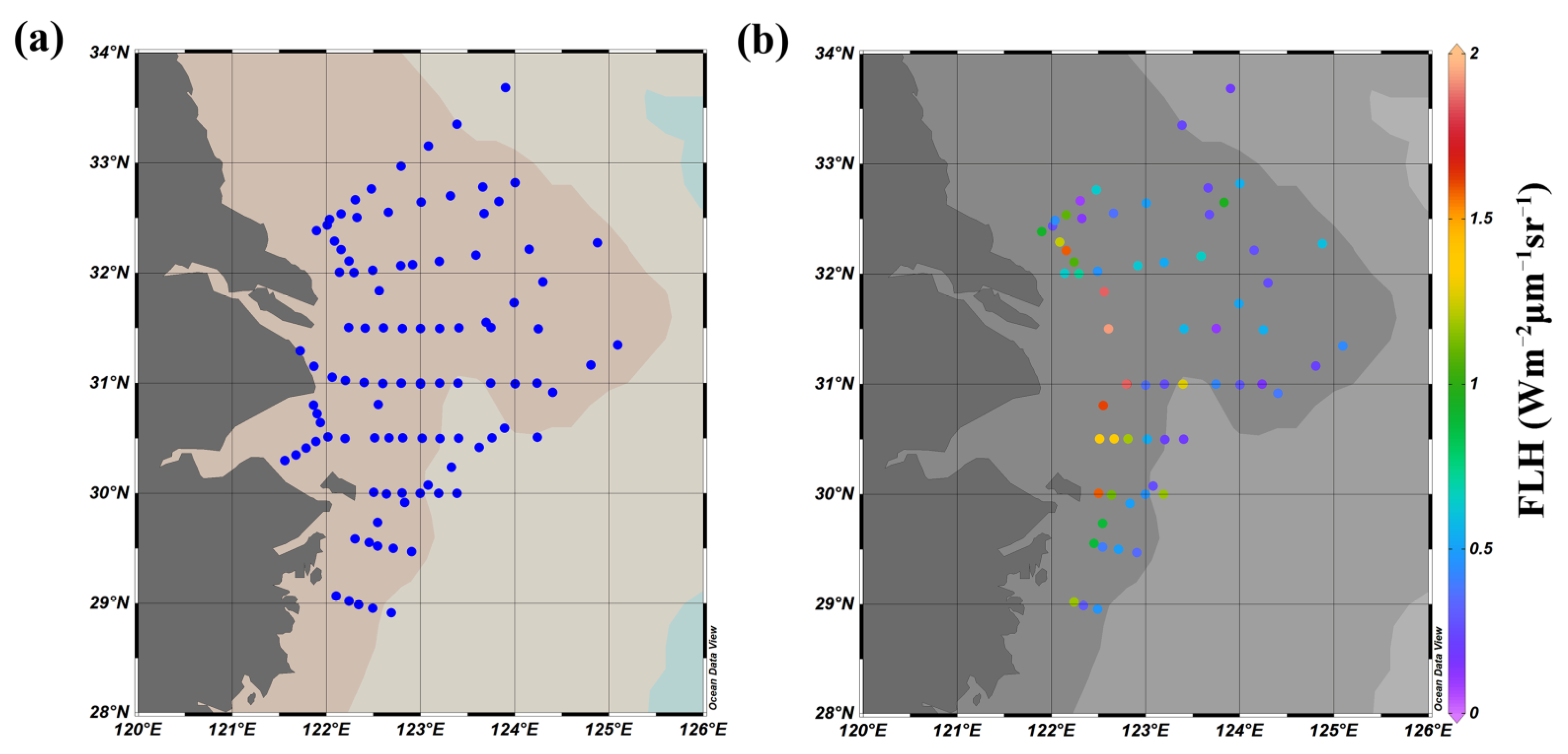
2.2. In Situ Data
2.3. Fluorescence Signal Calculation
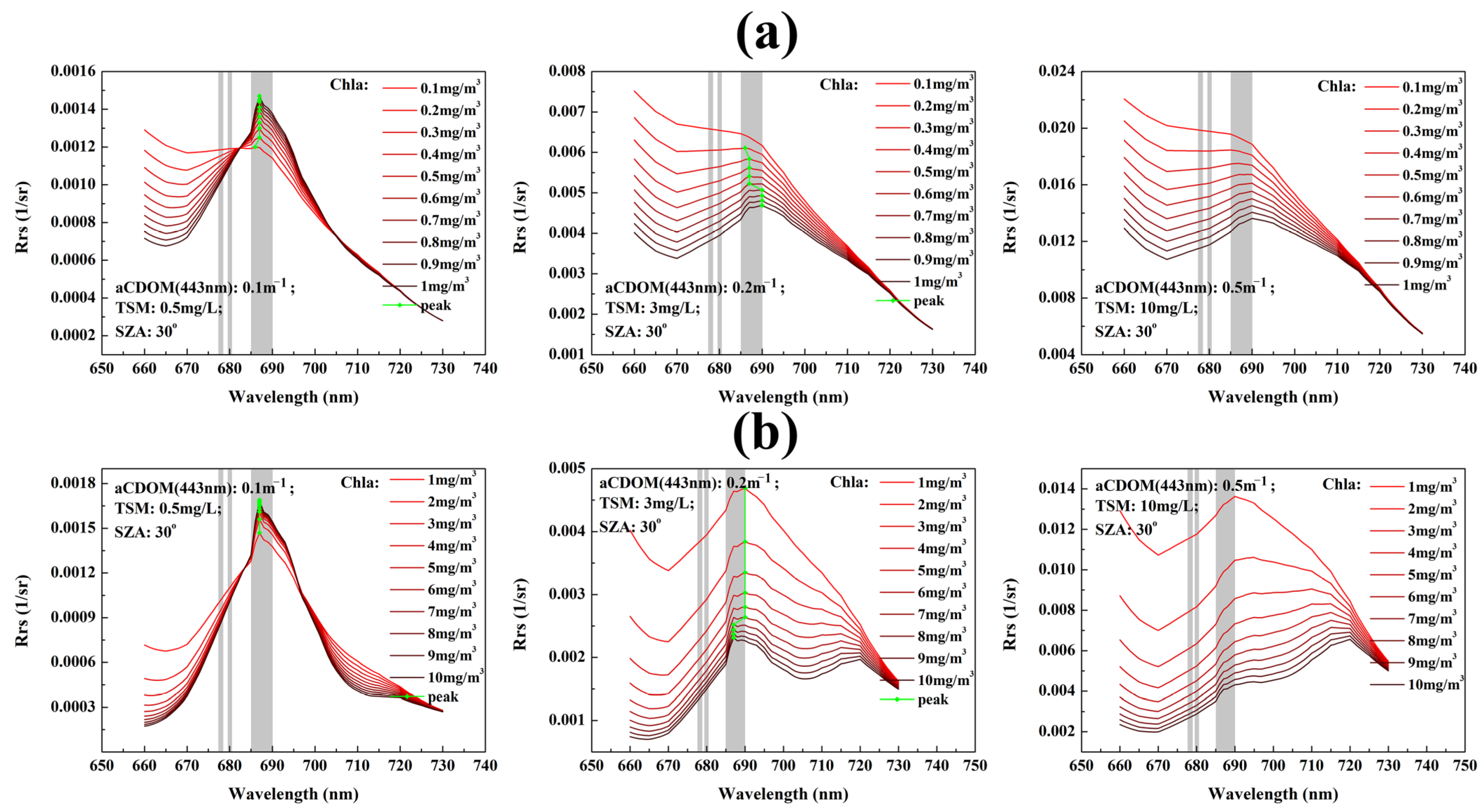
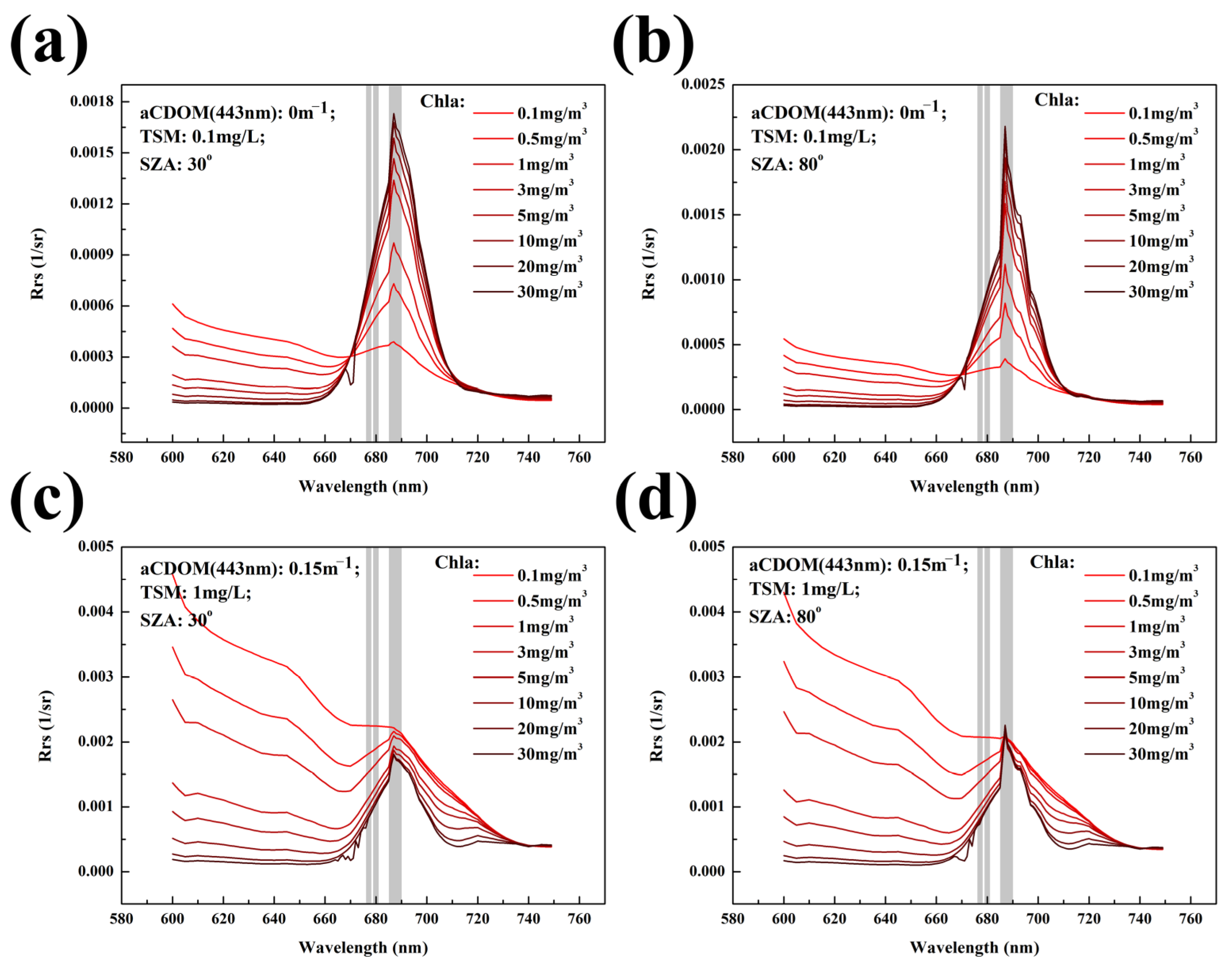
2.4. Radiative Transfer Simulations
2.5. Evaluation of Performance
- The percentages of valid pixels in the 3 × 3 box (excluding land pixels) were first checked. If the percentage was >50%, the box was adopted for the following quality assessment.
- The means and standard deviations (SDs) of valid values within the box were calculated. We discarded pixels with values outside the range of mean ± 1.5 SD.
- The means and SDs for the remaining valid pixels were recalculated and the coefficients of variation (CVs) were determined (where CV = SD/mean) to test spatial heterogeneity. If CV was <0.15, the box was adopted for matching the measured data with satellite data.
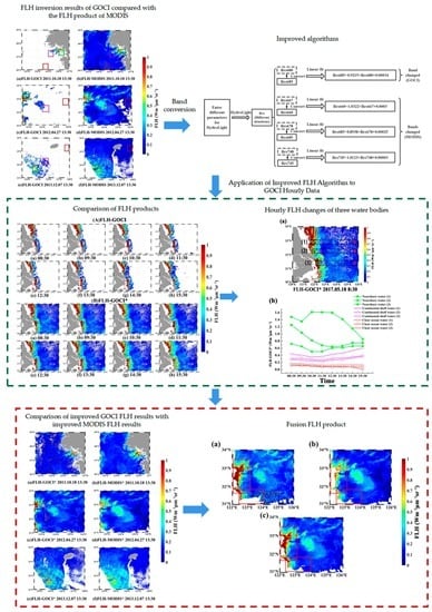
3. Establishment of the FLH Algorithm for GOCI
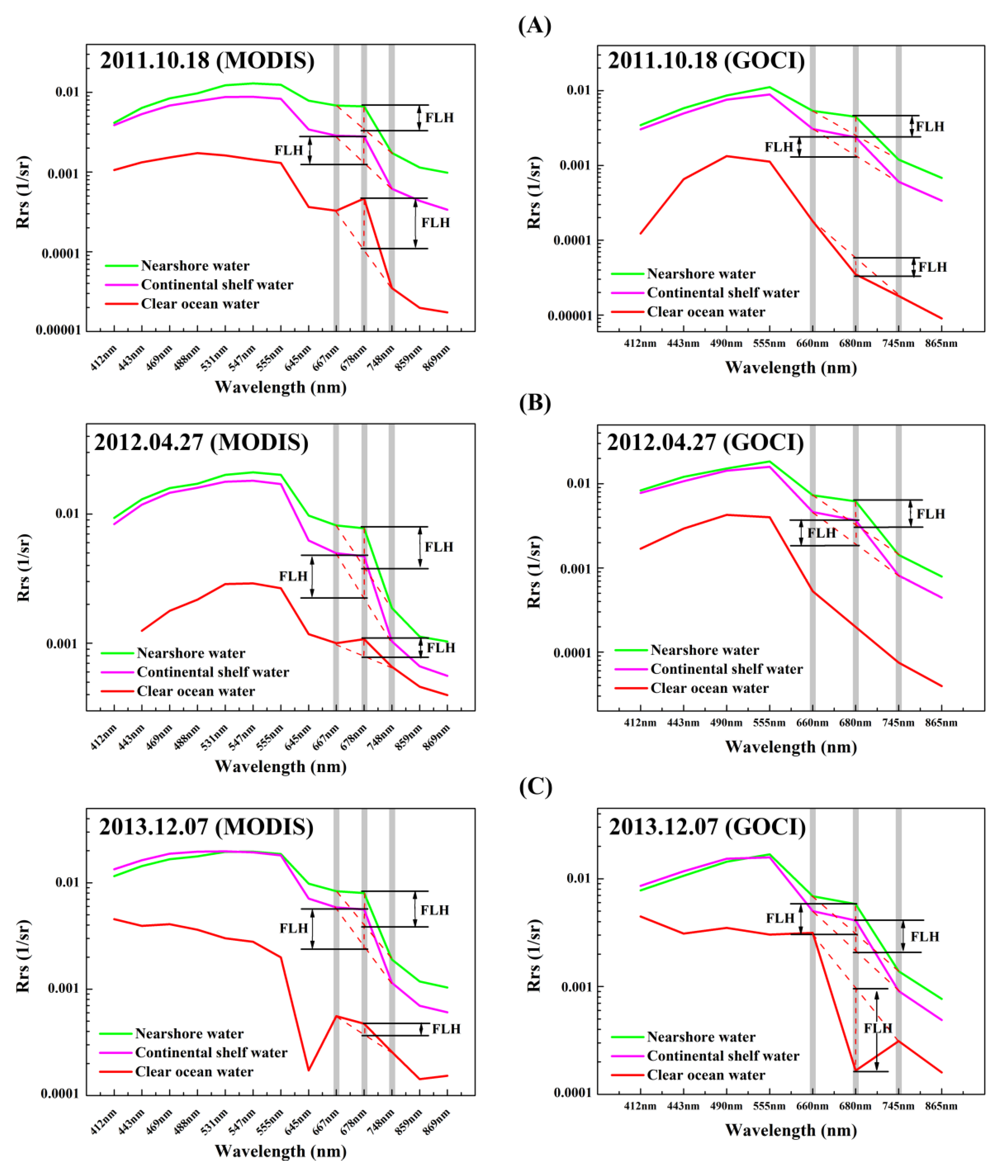
3.1. Analysis of GOCI and MODIS Chlorophyll Fluorescence Signals
3.2. Fluorescence Signal for Different Water Bodies
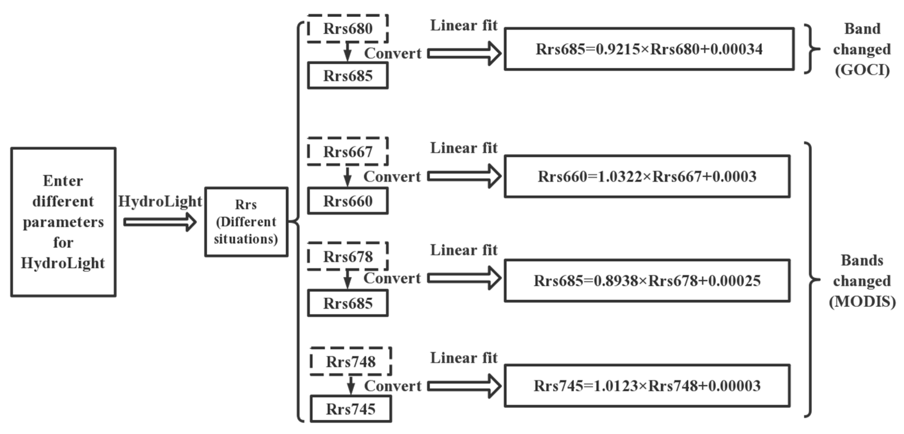
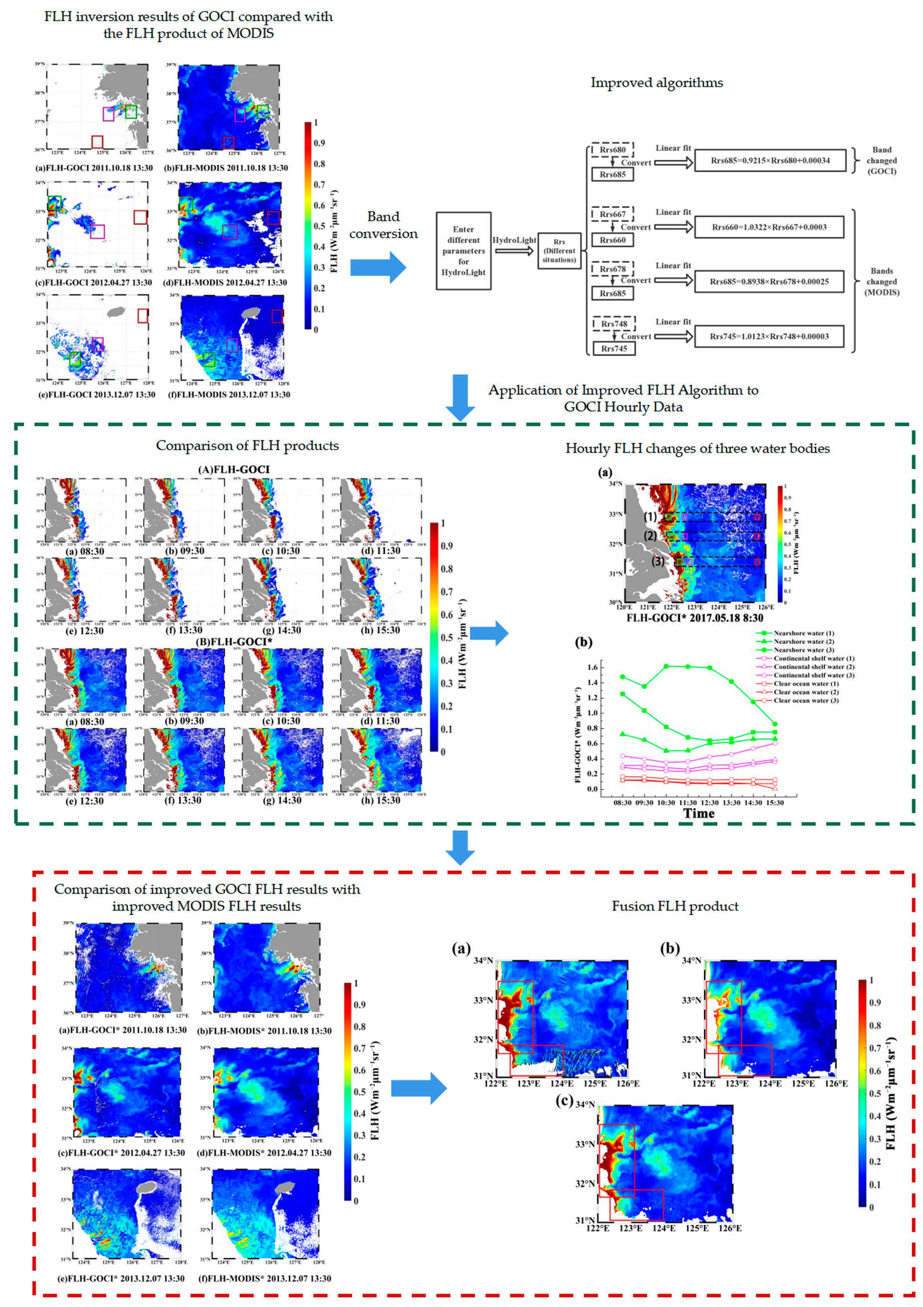
3.3. Band Conversion Method
4. Results and Discussion
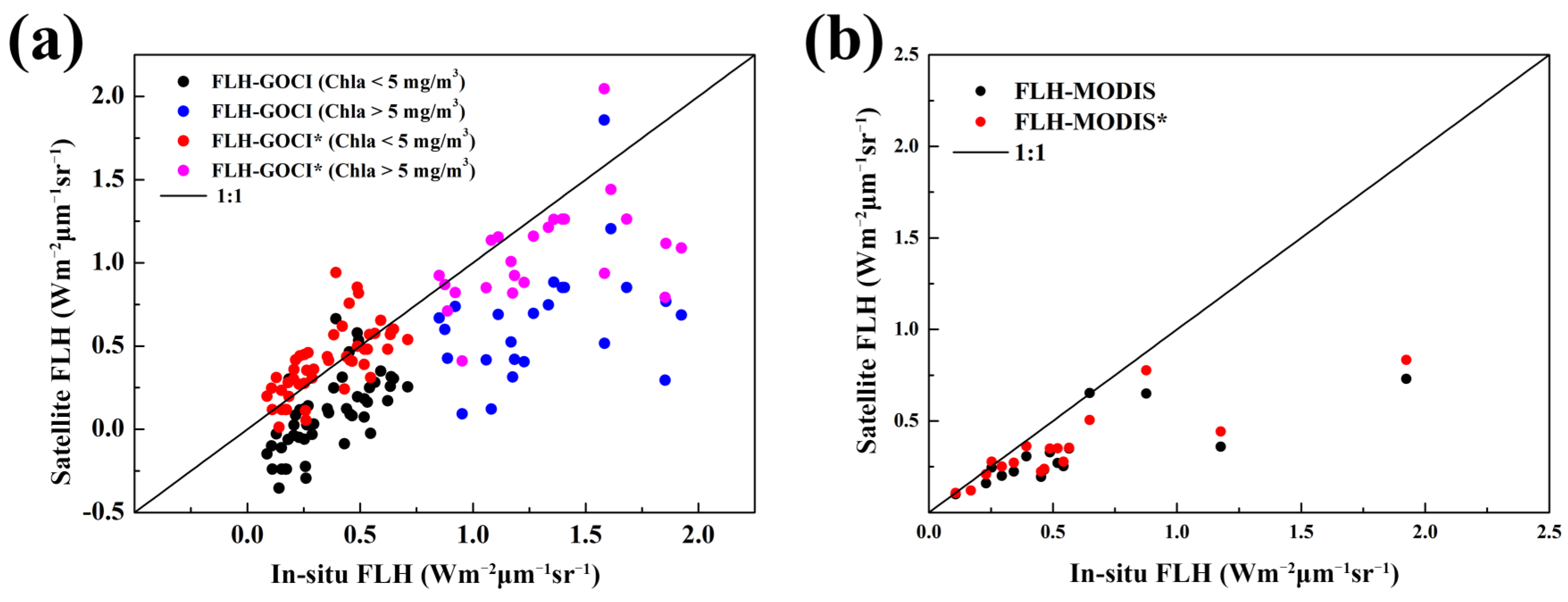
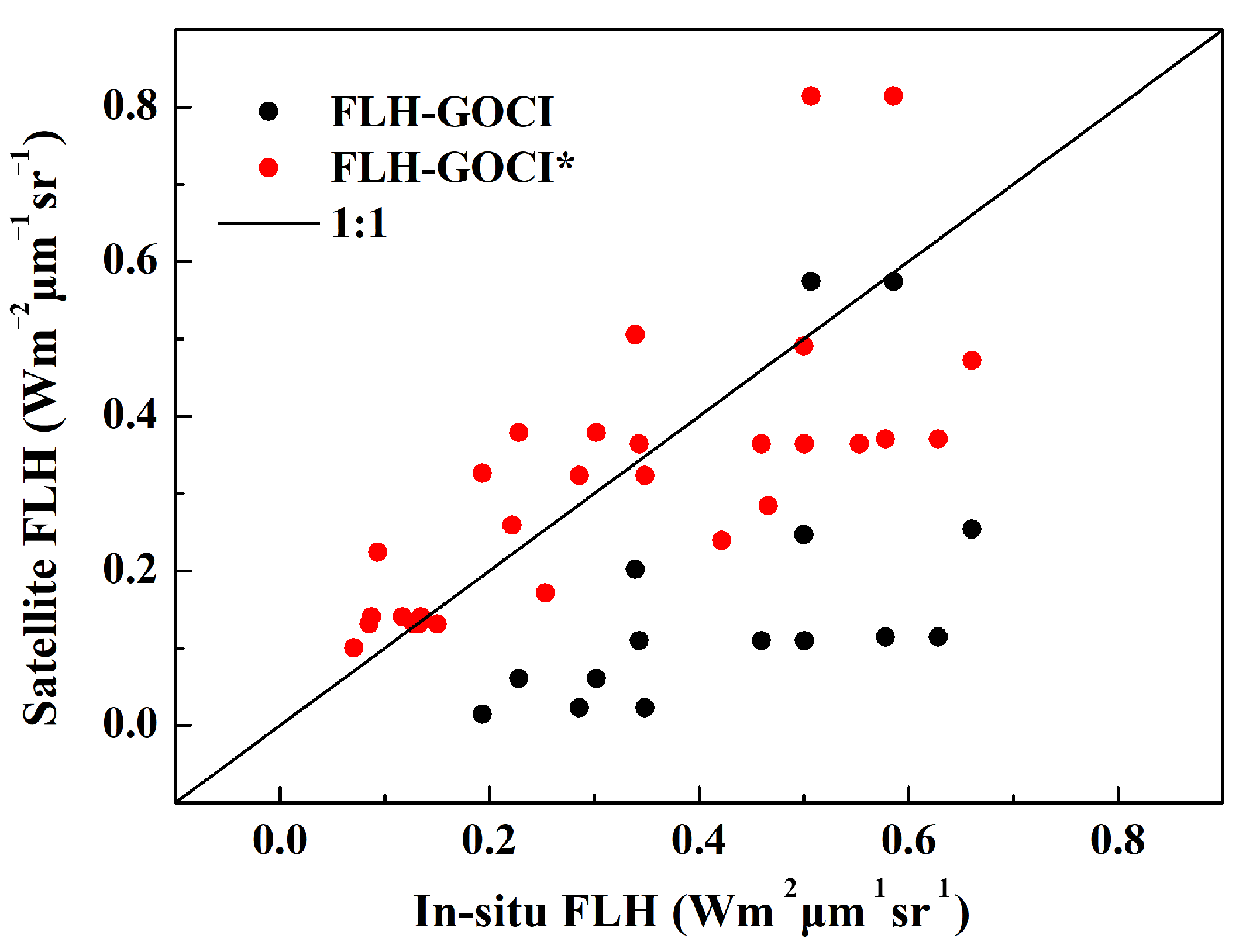
4.1. Algorithm Verification
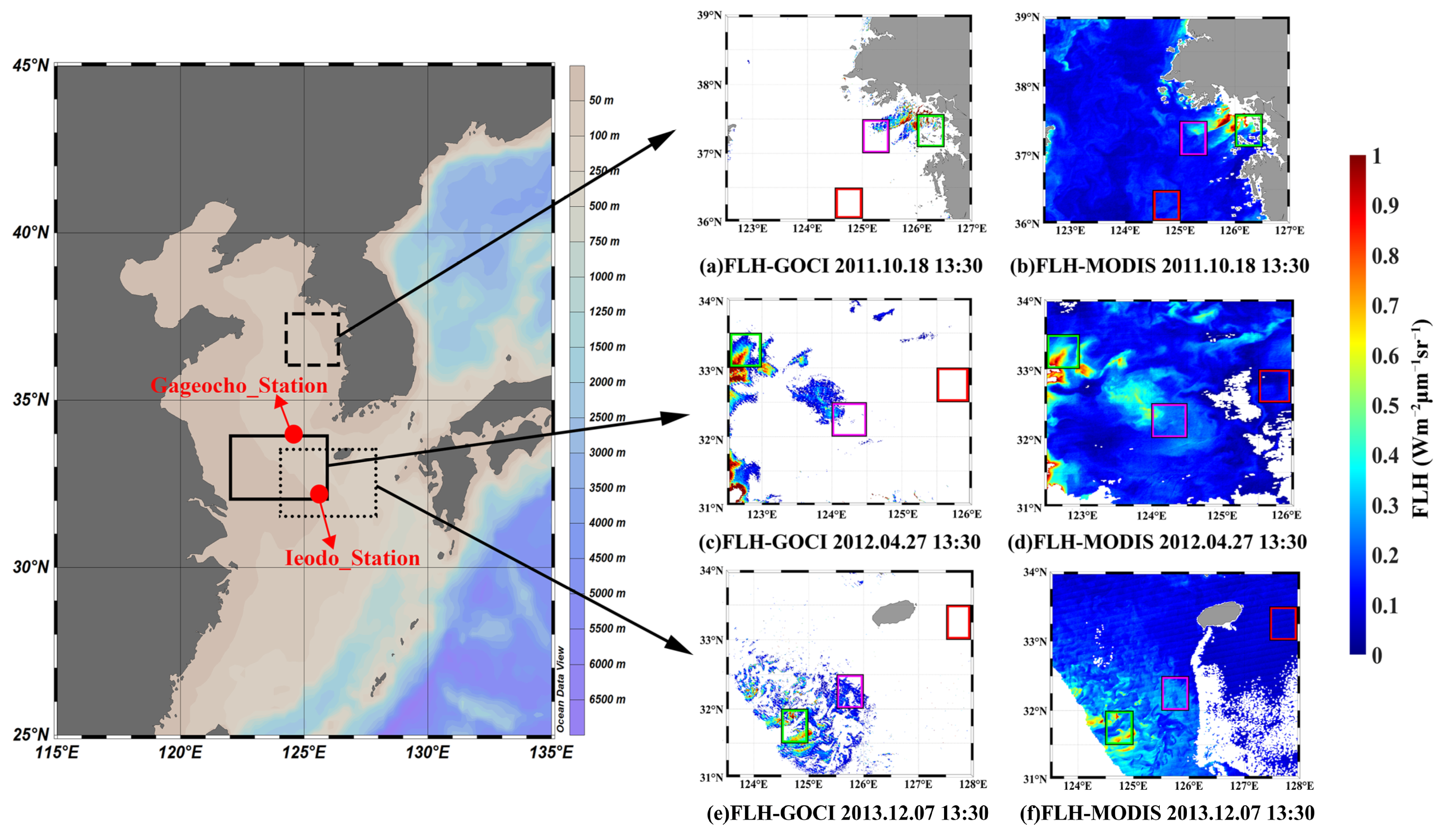
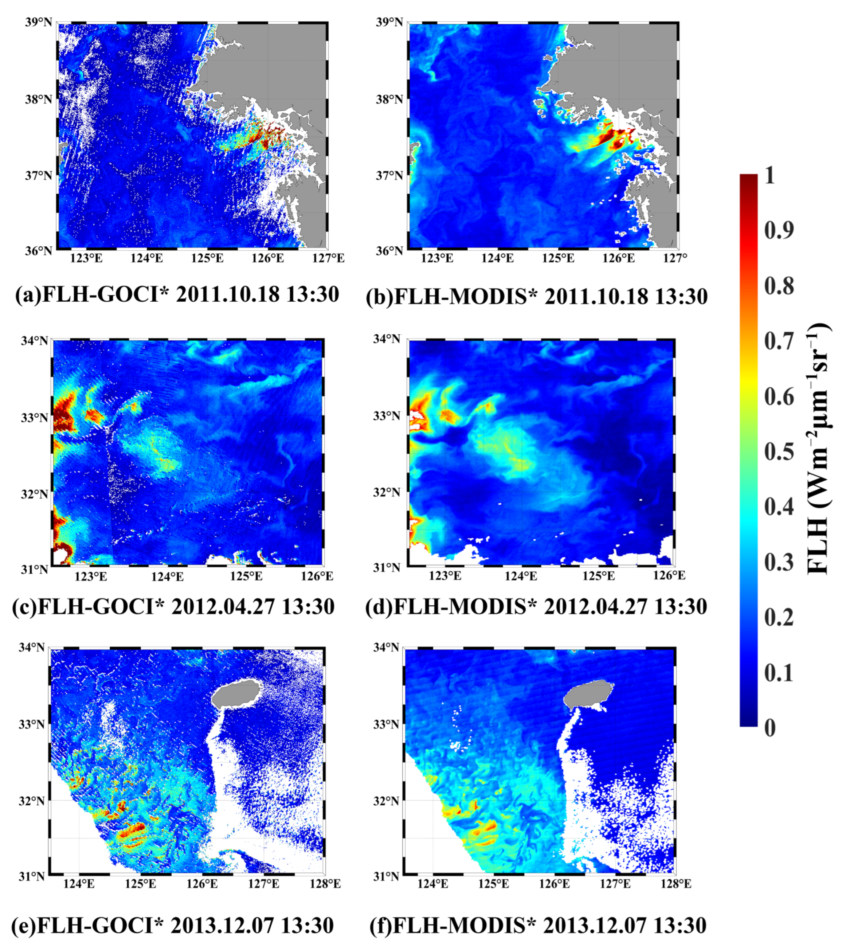
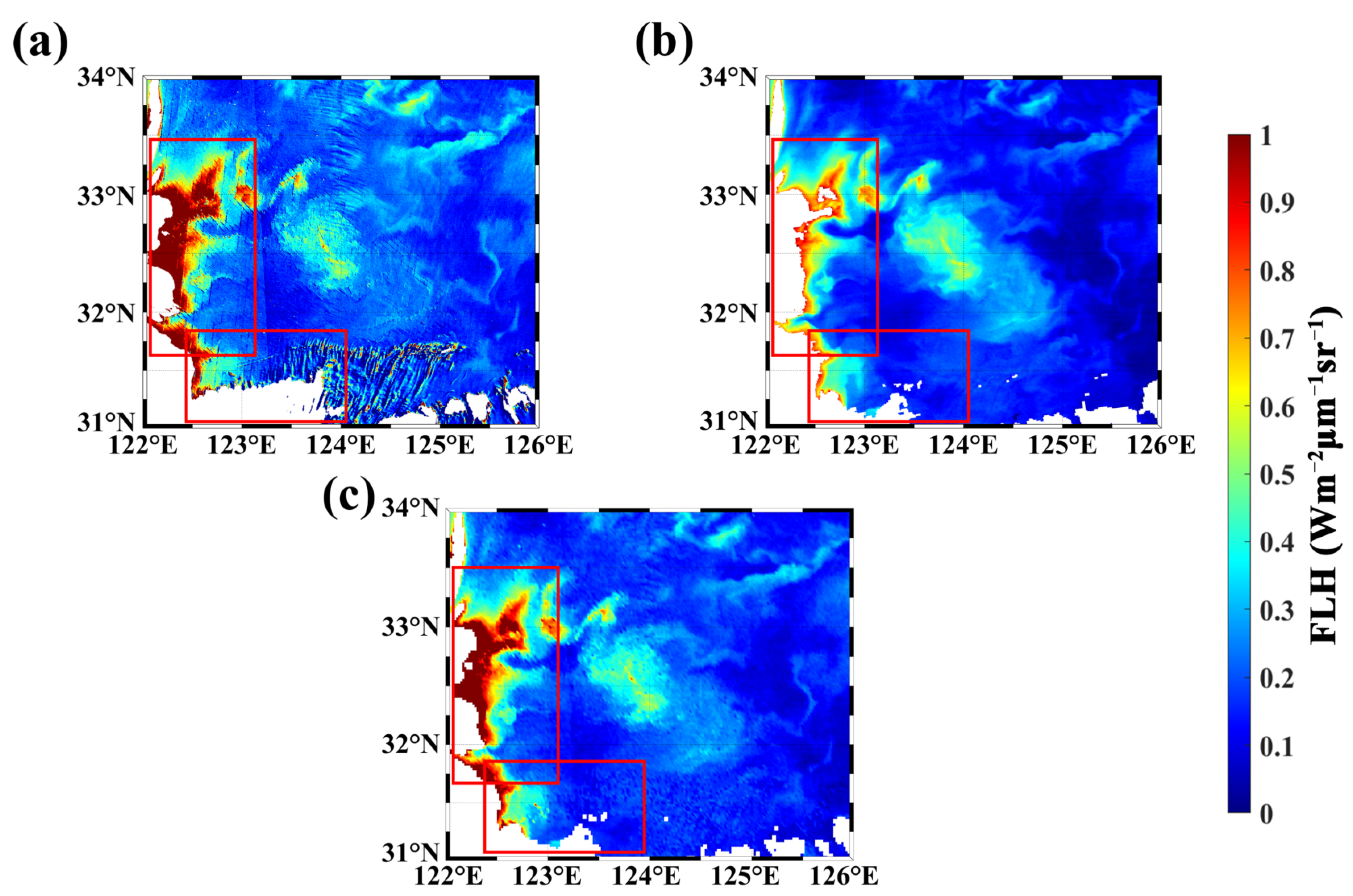
4.2. Cross-Comparison of GOCI and MODIS FLH Products
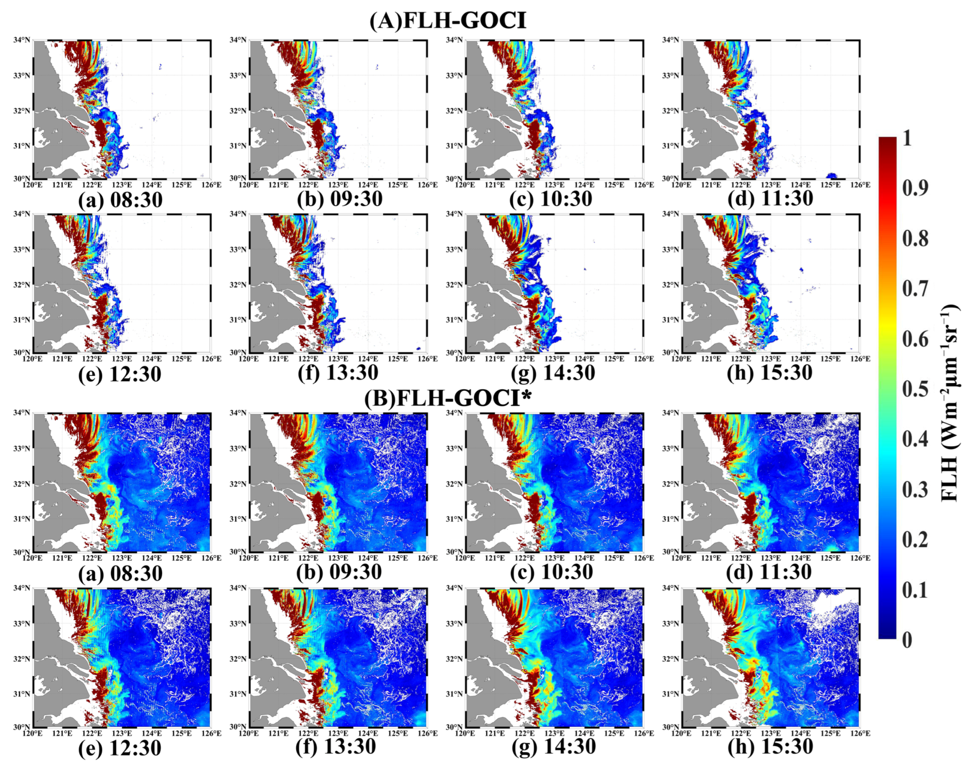
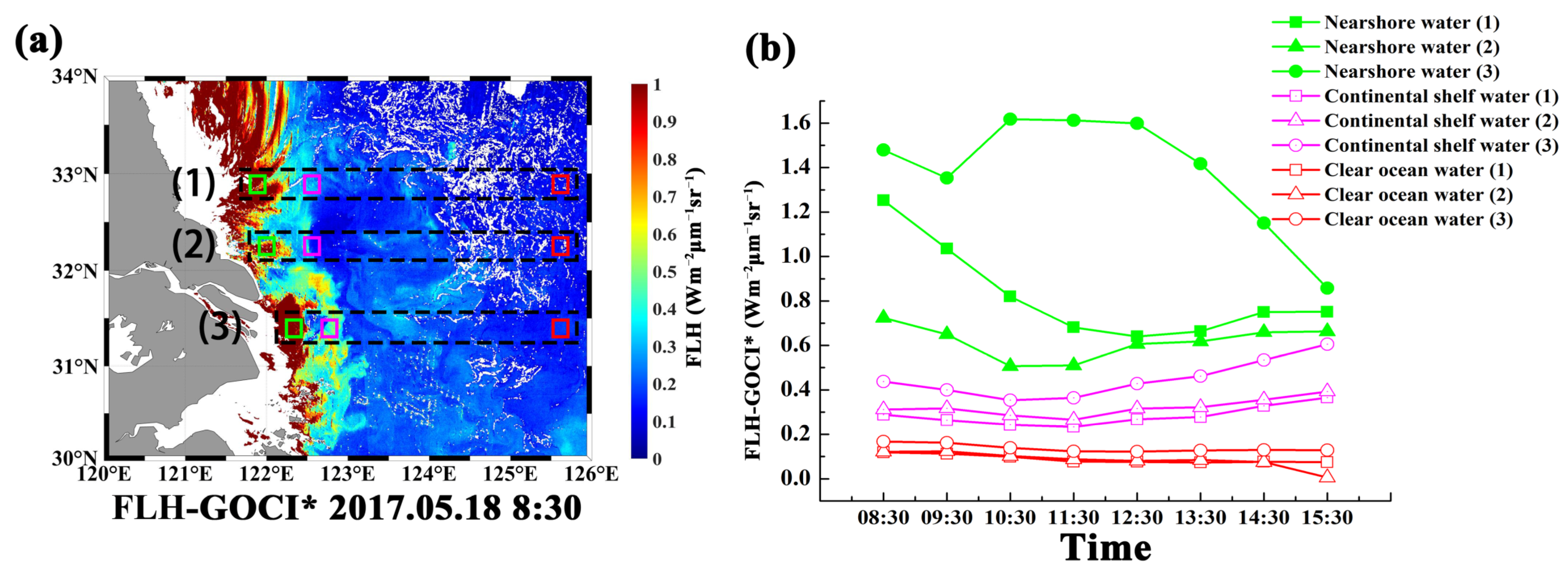
4.3. Application of Improved FLH Algorithm to GOCI Hourly Data
5. Conclusions
Author Contributions
Funding
Data Availability Statement
Acknowledgments
Conflicts of Interest
Appendix A
References
- Xing, X.G.; Zhao, D.Z.; Liu, Y.G.; Yang, J.H.; Wang, L. An overview of remote sensing of chlorophyll fluorescence. Ocean Sci. J. 2007, 42, 49–59. [Google Scholar] [CrossRef] [Green Version]
- Valentini, R.; Cecchi, G.; Mazzinghi, P.; Mugnozza, G.S.; Agati, G.; Bazzani, M.; De Angelis, P.; Fusi, F.; Matteucci, G.; Raimondi, V. Remote sensing of chlorophyll a fluorescence of vegetation canopies: 2. Physiological significance of fluorescence signal in response to environmental stresses. Remote Sens. Environ. 1994, 47, 29–35. [Google Scholar] [CrossRef]
- Rao, Y.U.; Nagamani, P.V.; Baranval, N.K.; Rao, P.R.; Rao, T.D.V.P.; Choudury, S.B. Detection of phytoplankton blooms in the turbid coastal waters using satellite-derived fluorescence line height off Kakinada coast. J. Indian Soc. Remote Sens. 2019, 47, 1857–1864. [Google Scholar]
- Blondeau, P.D.; Gower, J.F.R.; Dekker, A.G.; Phinn, S.R.; Brando, V.E. A review of ocean color remote sensing methods and statistical techniques for the detection, mapping and analysis of phytoplankton blooms in coastal and open oceans. Prog. Oceanogr. 2014, 123, 123–144. [Google Scholar] [CrossRef] [Green Version]
- Shehhi, M.R.A.; Gherboudj, I.; Ghedira, H. Detection of algal blooms over optically complex waters of the Arabian Gulf and Sea of Oman using MODIS fluorescence data. Int. J. Remote Sens. 2019, 40, 3751–3771. [Google Scholar] [CrossRef]
- Morel, A.; Prieur, L. Analysis of variations in ocean color. Limnol. Oceanogr. 1977, 22, 709–722. [Google Scholar] [CrossRef]
- Gower, J.F.R.; Doerffer, R.; Borstad, G.A. Interpretation of the 685 nm peak in water-leaving radiance spectra in terms of fluorescence, absorption and scattering, and its observation by MERIS. Int. J. Remote Sens. 1999, 20, 1771–1786. [Google Scholar] [CrossRef]
- Letelier, R.M.; Abbott, M.R. An analysis of chlorophyll fluorescence algorithms for the moderate resolution imaging spectrometer (MODIS). Remote Sens. Environ. 1996, 58, 215–223. [Google Scholar] [CrossRef]
- Fiorani, L.; Okladnikov, I.G.; Palucci, A. First algorithm for chlorophyll-a retrieval from MODIS-Terra imagery of sun-induced fluorescence in the southern ocean. Int. J. Remote Sens. 2006, 27, 3615–3622. [Google Scholar] [CrossRef]
- Hoge, F.E.; Lyon, P.E.; Swift, R.N.; Yungel, J.K.; Esaias, W.E. Validation of Terra-MODIS phytoplankton chlorophyll fluorescence line height.initial airborne lidar results. Appl. Opt. 2003, 42, 2767–2771. [Google Scholar] [CrossRef]
- Gower, J.; King, S. Validation of chlorophyll fluorescence derived from MERIS on the west coast of Canada. Int. J. Remote Sens. 2013, 11, 1497–1504. [Google Scholar] [CrossRef]
- Son, Y.B.; Ishizaka, J.; Jeong, J.C.; Kim, H.C.; Lee, T. Cochlodinium polykrikoides red tide detection in the south Sea of Korea using spectral classification of MODIS data. Ocean Sci. J. 2011, 46, 239–263. [Google Scholar] [CrossRef]
- Behrenfeld, M.J.; Westberry, T.K.; Boss, E.S.; O’Malley, R.T.; Siegel, D.A.; Wiggert, J.D.; Franz, B.A.; McClain, C.R.; Feldman, G.C.; Doney, C.S.; et al. Satellite-detected fluorescence reveals global physiology of ocean phytoplankton. Biogeosciences 2009, 6, 779–794. [Google Scholar] [CrossRef] [Green Version]
- O’Malley, R.T.; Behrenfeld, M.J.; Westberry, T.K.; Milligan, A.J.; Shang, S.; Yan, J. Geostationary satellite observations of dynamic phytoplankton photophysiology. Geophys. Res. Lett. 2014, 41, 5052–5059. [Google Scholar] [CrossRef]
- Li, H.; He, X.; Bai, Y.; Shanmugam, P.; Huang, H. Atmospheric correction of geostationary satellite ocean color data under high solar zenith angles in open oceans. Remote Sens. Environ. 2020, 249, 112022. [Google Scholar] [CrossRef]
- Li, H.; He, X.; Shanmugam, P.; Bai, Y.; Wang, D.; Huang, H.; Zhu, Q.; Gong, F. Radiometric sensitivity and signal detectability of ocean color satellite sensor under high solar zenith angles. IEEE Trans. Geosci. Remote 2019, 57, 8492–8505. [Google Scholar] [CrossRef]
- Son, Y.B.; Kang, Y.H.; Ryu, J.H. Monitoring red tide in south Sea of Korea (SSK) using the geostationary ocean color imager (GOCI). Korean J. Remote Sens. 2012, 28, 531–548. [Google Scholar] [CrossRef]
- Kim, W.; Moon, J.E.; Park, Y.J.; Ishizaka, J. Evaluation of chlorophyll retrievals from Geostationary Ocean Color Imager (GOCI) for the north-east Asian region. Remote Sens. Environ. 2016, 184, 482–495. [Google Scholar] [CrossRef]
- Gohin, F.; Druon, J.N.; Lampert, L. A five channel chlorophyll concentration algorithm applied to SeaWiFS data processed by SeaDAS in coastal waters. Int. J. Remote Sens. 2002, 23, 1639–1661. [Google Scholar] [CrossRef]
- Bailey, S.W.; Werdell, P.J. A multi-sensor approach for the on-orbit validation of ocean color satellite data products. Remote Sens. Environ. 2006, 102, 12–23. [Google Scholar] [CrossRef]
- He, X.; Bai, Y.; Pan, D.; Huang, N.; Dong, X.; Chen, J.; Chen, C.-T.A.; Cui, Q. Using geostationary satellite ocean color data to map the diurnal dynamics of suspended particulate matter in coastal waters. Remote Sens. Environ. 2013, 133, 225–239. [Google Scholar] [CrossRef]
- Le, C.; Hu, C.; Cannizzaro, J.; English, D.; Muller-Karger, F.; Lee, Z. Evaluation of chlorophyll-a remote sensing algorithms for an optically complex estuary. Remote Sens. Environ. 2013, 129, 75–89. [Google Scholar] [CrossRef]
- Mobley, C.D. Estimation of the remote-sensing reflectance from above-surface measurements. Appl. Opt. 1999, 38, 7442–7455. [Google Scholar] [CrossRef] [PubMed]
- Pope, R.M.; Fry, E.S. Absorption spectrum (380–700 nm) of pure water. II. Integrating cavity measurements. Appl. Opt. 1997, 36, 8710–8723. [Google Scholar] [CrossRef] [PubMed]
- Wei, J.; Lee, Z.; Pahlevan, N.; Lewis, M.R. Transmittance of upwelling radiance at the sea surface measured in the field. Ocean Remote Sens. Monit. Space 2014, 9261, 24–30. [Google Scholar]
- Smith, R.C.; Austin, R.W.; Petzold, T.J. Volume-Scattering Functions in Ocean Waters; Springer: Berlin/Heidelberg, Germany, 1974; pp. 61–72. [Google Scholar]
- He, X.Q.; Bai, Y.; Pan, D.L.; Chen, C.-T.A.; Cheng, Q.; Wang, D.; Gong, F. Satellite views of the seasonal and interannual variability of phytoplankton blooms in the eastern China seas over the past 14 yr (1998–2011). Biogeosciences 2013, 10, 4721–4739. [Google Scholar] [CrossRef] [Green Version]
- Xing, X.G. Remote-Sensing Study of Chlorophyll Fluorescence. Ph.D. Thesis, Chinese Marine University, Qingdao, China, 2008. [Google Scholar]
- Li, H.; He, X.Q.; Shanmugam, P.; Bai, Y.; Wang, D.; Huang, H.; Zhu, Q.; Gong, F. Semi-analytical algorithms of ocean color remote sensing under high solar zenith angles. Opt. Express 2019, 27, A800–A817. [Google Scholar] [CrossRef]
- Li, H.; He, X.Q.; Bai, Y.; Chen, X.; Gong, F.; Zhu, Q.; Hu, Z. Assessment of satellite-based chlorophyll-a retrieval algorithms for high solar zenith angle conditions. J. Appl. Remote Sens. 2017, 11, 012004. [Google Scholar] [CrossRef]
- Hall, N.S.; Whipple, A.C.; Paerl, H.W. Vertical spatio-temporal patterns of phytoplankton due to migration behaviors in two shallow, microtidal estuaries: Influence on phytoplankton function and structure. Estuar. Coast. Shelf Sci. 2015, 162, 7–21. [Google Scholar] [CrossRef] [Green Version]


| Parameter | Values |
|---|---|
| Chla (mg/m3) | 0.1; 0.2; 0.5; 1; 2; 5; 10; 20; 50; 100; 150; 300 |
| TSM (mg/L) | 0.1; 0.2; 0.5; 1; 2; 5; 10; 20; 50; 100; 150; 300 |
| aCDOM(443 nm) (m−1) | 0.1; 0.2; 0.5; 1; 2; 5; 10 |
| SZA (°) | 0; 20; 40; 60; 70; 80 |
| Water Condition | Parameter | ||
|---|---|---|---|
| Chla (mg/m3) | TSM (mg/L) | aCDOM(443 nm) (m−1) | |
| Clear ocean water | 0.1 | 0.1 | 0 |
| Continental shelf water | 1 | 1 | 0.15 |
| Nearshore water | 5 | 1 | 0.2 |
| Algorithm | N | R2 | RMSD (sr−1) | APD (%) | RPD (%) |
|---|---|---|---|---|---|
| FLH-GOCI (Chla < 5 mg/m3) | 52 | 0.61 | 0.32 | 105.72 | −35.02 |
| FLH-GOCI* (Chla < 5 mg/m3) | 52 | 0.67 | 0.16 | 41.92 | 19.09 |
| FLH-GOCI (Chla > 5 mg/m3) | 25 | 0.14 | 0.77 | 51.60 | −50.21 |
| FLH-GOCI* (Chla > 5 mg/m3) | 25 | 0.20 | 0.43 | 22.02 | −18.29 |
| FLH-MODIS | 17 | 0.63 | 0.39 | 35.10 | −35.02 |
| FLH-MODIS* | 17 | 0.74 | 0.35 | 28.85 | −27.75 |
| Algorithm | N | R2 | RMSD (sr−1) | APD (%) | RPD (%) |
|---|---|---|---|---|---|
| FLH-GOCI | 15 | 0.29 | 0.30 | 65.60 | −63.83 |
| FLH-GOCI* | 30 | 0.54 | 0.13 | 33.10 | 11.40 |
| Time | 8:30 | 9:30 | 10:30 | 11:30 | 12:30 | 13:30 | 14:30 | 15:30 | 8-Scene Average |
|---|---|---|---|---|---|---|---|---|---|
| FLH-GOCI* | 65.87 | 67.22 | 67.03 | 65.65 | 67.00 | 68.35 | 68.12 | 64.60 | 66.73 |
| FLH-GOCI | 14.27 | 13.34 | 12.18 | 12.47 | 13.84 | 15.53 | 17.69 | 18.93 | 14.78 |
Publisher’s Note: MDPI stays neutral with regard to jurisdictional claims in published maps and institutional affiliations. |
© 2022 by the authors. Licensee MDPI, Basel, Switzerland. This article is an open access article distributed under the terms and conditions of the Creative Commons Attribution (CC BY) license (https://creativecommons.org/licenses/by/4.0/).
Share and Cite
Zhao, M.; Bai, Y.; Li, H.; He, X.; Gong, F.; Li, T. Fluorescence Line Height Extraction Algorithm for the Geostationary Ocean Color Imager. Remote Sens. 2022, 14, 2511. https://doi.org/10.3390/rs14112511
Zhao M, Bai Y, Li H, He X, Gong F, Li T. Fluorescence Line Height Extraction Algorithm for the Geostationary Ocean Color Imager. Remote Sensing. 2022; 14(11):2511. https://doi.org/10.3390/rs14112511
Chicago/Turabian StyleZhao, Min, Yan Bai, Hao Li, Xianqiang He, Fang Gong, and Teng Li. 2022. "Fluorescence Line Height Extraction Algorithm for the Geostationary Ocean Color Imager" Remote Sensing 14, no. 11: 2511. https://doi.org/10.3390/rs14112511
APA StyleZhao, M., Bai, Y., Li, H., He, X., Gong, F., & Li, T. (2022). Fluorescence Line Height Extraction Algorithm for the Geostationary Ocean Color Imager. Remote Sensing, 14(11), 2511. https://doi.org/10.3390/rs14112511