Reference-Based Multi-Level Features Fusion Deblurring Network for Optical Remote Sensing Images

Abstract

Blind image deblurring is a long-standing challenge in remote sensing image restoration tasks. It aims to recover a latent sharp image from a blurry image while the blur kernel is unknown. To solve this problem, many image priors-based algorithms and learning-based algorithms have been proposed. However, most of these methods are based on a single blurry image. Due to the lack of high frequency information, the images restored by these algorithms still have some deficiencies in edge and texture details. In this work, we propose a novel deep learning model named Reference-Based Multi-Level Features Fusion Deblurring Network (Ref-MFFDN), which registers the reference image and the blurry image in the multi-level feature space and transfers the high-quality textures from registered reference features to assist image deblurring. Comparative experiments on the testing set prove that our Ref-MFFDN outperforms many state-of-the-art single image deblurring approaches in both quantitative evaluation and visual results, which indicates the effectiveness of using reference images in remote sensing image deblurring tasks. More ablation experiments demonstrates the robustness of Ref-MFFDN to the input image size, the effectiveness of multi-level features fusion network (MFFN) and the effect of different feature levels in multi-feature extractor (MFE) on algorithm performance.

1. Introduction

High-quailty remote sensing images have played an important role in change detection [1], urban planning [2,3], environmental monitoring [4,5] and so on. However, affected by many factors such as camera shake, lens defocus and atmospheric disturbance, the observed images often suffer from image quality degradation and loss of important texture information. Image deblurring is a long-standing problem in remote sensing tasks. When the blurring is uniform and spatially invariant, it can be expressed as:

$$B=I*K+N,$$

(1)

where B, I, K and N denotes the blurry image, the latent sharp image, the blur kernel and additive noise, respectively. The operation ∗ stands for the discrete convolution.

Deblurring methods are generally divided into two types: non-blind image deblurring and blind image deblurring. Non-blind deblurring assumes that the blur kernel is known or has been estimated beforehand, while blind deblurring estimates both blur kernel and latent sharp image or derives the latent sharp image directly.

Basically, deblurring is a highly ill-posed problem with countless conditional solutions. To make this problem well-posed, many image priors are considered, such as gradient prior [6,7,8], dark channel prior [9,10], local minimal intensity prior [11], local binary pattern prior [12], latent structure prior [13] and so on. However, most image priors lack generalization since they are based on limited observations of specific scenes. Therefore, it is worthwhile to explore more general image priors. To ameliorate this issue, many deblurring methods based on deep learning are proposed, such as the works of Sun [14], Nah [15] and Kupyn [16]. Among these deep learning-based methods, images harvested by convolutional neural network-based (CNN-based) methods usually lack textures. Generative adversarial network-based (GAN-based) methods can provide detailed structures, but sometimes may generate fake textures and artifacts.

To reconstruct the fine and realistic textures, some research on image Super-Resolution (SR) transferred high-resolution (HR) textures from a given reference image to a low-resolution (LR) image [17,18,19,20,21]. These reference-based SR (RefSR) methods provide a feasible way for image deblurring. For better algorithm performance, a strong correlation is usually required between the reference image and the input image. Compared with ordinary optical images, strongly correlated reference images are easier to obtain in remote sensing images. Possible methods are as follows:

• As a publicly available remote sensing image platform, Google Earth provides high-resolution satellite images from around the world. It is feasible to pick up images from Google Earth as reference images.
• The imaging process of many satellites is periodic and a large number of images of the same region at different time are accumulated, which can be used as reference images.

Although highly correlated reference images can be obtained in remote sensing tasks, alignment between the blurry image and the reference image is still necessary because a difference still exists in some scenes caused by factors such as different shooting viewpoints, deviations in geographic coordinates, different atmospheric conditions and the effect of the time change. More specifically, how to extract the texture features matching the blurry image from the reference image is the key to the reference-based remote sensing deblurring algorithm.

To address this problem, we propose a novel Reference-Based Multi-Level Features Fusion Deblurring Network (Ref-MFFDN). The Ref-MFFDN is mainly divided into three modules: multi-level features fusion network (MFFN), encoder network (EN) and decoder network (DN). Moreover, the MFFN module mainly consists of two parts: multi-level features extractor (MFE) and feature fusion (FF). More specifically, multi-level features of blurry images and reference images are extracted by MFE with shared weights. Then, in FF, these paired features are further calculated with hard attention maps and soft attention maps to generate fused features. Finally, the fused features will be concatenated with the features of blurry images extracted by EN and be fed into DN to harvest latent sharp images. The main contributions of this paper are:

• To the best of our knowledge, we are one of the first to explore reference-based deblurring method on remote sensing images.
• We designed a novel MFFN module, which registers the reference image and the blurry image in the multi-level feature space and transfers the high-quality textures from registered reference features to assist image deblurring. Furthermore, the effectiveness of MFFN is demonstrated by the ablation experiments.
• We construct a dataset for blind remote sensing image deblurring with data from the United States Department of Agriculture (USDA). In the testing set, our algorithm outperforms all comparative methods in both quantitative evaluation and visual results, which proves the great potential of the reference-based deblurring approach in the field of remote sensing.

The rest of this article is organized as follows. We introduce the related work in Section 2 and give a detailed description of the proposed Ref-MFFDN, loss functions, dataset and metrics in Section 3. Experimental results and discussion are provided in Section 4. In Section 5, we conclude our work.

2. Related Works

In this section, we briefly review previous works of learning-based blind deblurring algorithms and reference-based SR algorithms which provide a feasible idea for our work.

2.1. Learning-Based Blind Deblurring Algorithms

Learning-based blind deblurring algorithms have developed rapidly in recent years. Sun et al. [14] proposed a convolutional neural network (CNN) model to estimate the motion blur at each image patch and then remove non-uniform motion blur in the whole image. Nah et al. [15] proposed a multiscale CNN and multiscale loss function to restore latent sharp images, following a coarse-to-fine strategy. Xu et al. [22] proposed a two-stage model based on CNN to suppress extraneous details and enhance sharp edges. Zhang et al. [23] proposed a novel end-to-end trainable spatially variant RNN for dynamic scene deblurring. Kupyn et al. [16] proposed an image deblurring algorithm based on generative adversarial network which can generate more realistic details in deblurred image. Li et al. [24] proposed a neural network architecture based on algorithm unrolling technique, which improves the image restoration performance and operation speed. Suin et al. [25] proposed an efficient deblurring design built on new convolutional modules that learn the transformation of features using global attention and adaptive local filters. However, the above algorithms are all based on a single blurry image. Due to the lack of high frequency information, the images restored by these algorithms still have some deficiencies in edge and texture details.

2.2. Reference-Based SR Algorithms

In recent years, RefSR algorithms have been greatly developed which provide a feasible way for image deblurring. These methods introduce additional high-frequency details from reference images to help reconstruct high-resolution images with fine textures.

Some existing RefSR algorithms [21,26,27] adopt the method called image alignment to align the LR and Ref image. Yue et al. [26] proposed a novel matching method to combine the high-level matching and low-level matching. They first aligned the reference images with the up-sampled LR image through a global registration, which identified the corresponding regions and reduced the mismatching. Then, they proposed a structure-aware matching criterion and adaptive block sizes to improve the mapping accuracy between LR and HR patches. Zheng et al. [27] proposed a fully convolutional cross-scale alignment module to align the reference image information with the LR image spatially. They adopted cross-scale warping to handle non-rigid objects in images and adopted a cross-scale flow estimator to align the LR and Ref image at multiple scale. Dong et al. [21] employed deformable convolutions to align gradient-guided Ref and LR features and proposed a relevance attention module to transfer the aligned reference features in a multiscale way. These image alignment methods are intuitive and convenient, but their performance rely on the alignment quality between reference image and LR images.

Patch alignment is another RefSR method [19,20,28] which aims to find the most relevant Ref feature for each LR patch. Zheng et al. [28] regarded the feature learning as a classification problem and designed a cross-scale correspondence network to achieve cross-scale patch alignment between reference and LR image. Zhang et al. [19] employed a pretrained VGG network to extract Ref and LR features and then calculated and compared the similarity between reference features and LR features patch-wisely to swap similar texture features. Yang et al. [20] proposed a relevance embedding module to compute the relevance between the LR and Ref image in the feature space. In this module, a hard attention map and a soft attention map were adopted to transform and fuse HR features from Ref images into LR features. When there are significant differences between the reference image and the blurred image, such as misalignment and environment changes, patch alignment can achieve better performance than image alignment. However, this method is usually computationally intensive and time-consuming.

Inspired by the above RefSR algorithms, we try to introduce the high-frequency information of the reference image to assist image deblurring. Due to environmental changes, urban planning and other factors, different scenes exist in the reference image and the blurry image. Thus, we adopt patch alignment strategy and propose an MFFN module to register the feature between the reference image and the blurred image. Then, we adopt the encoder-decoder framework to achieve image deblurring.

3. Materials and Methods

In this section, we introduce the proposed Reference-Based Multi-Level Features Fusion Deblurring Network (Ref-MFFDN). The overall architecture is illustrated in Figure 1. The Ref-MFFDN is mainly divided into three modules: multi-level features fusion network (MFFN), encoder network (EN) and decoder network (DN). These modules are discussed in Section 3.1, Section 3.2 and Section 3.3 separately. The detailed structure for each module is introduced in Appendix A. A set of loss functions for optimizing the proposal network are explained in Section 3.4.

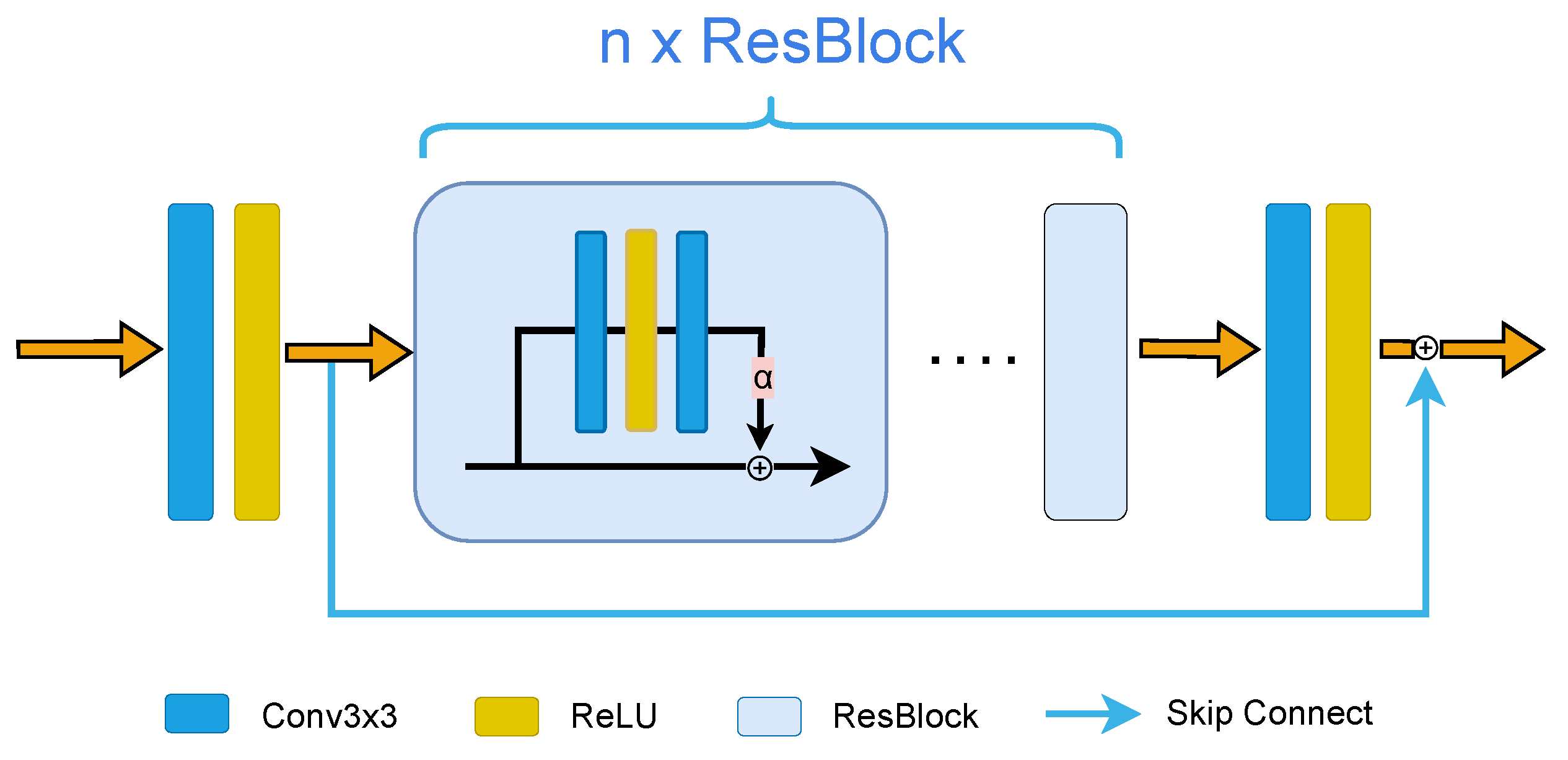
3.1. Multi-Level Features Fusion Network

To efficiently transfer relevant and high-quality texture information from reference images into blurry images, we design the MFFN module. The MFFN module mainly consists of two parts: multi-level features extractor (MFE) and feature fusion (FF).

Multi-level features extractor: The MFE module is used to extract the multi-level features of the reference image and the blurry image and its structure is shown in Figure 2. For a more accurate and efficient operation, we use the first four layers of the pretrained semantic feature extraction network VGG19 [29] to extract the first-level features of the input image. Let $\mathit{I}$ denote the input image. The operation can be expressed as:

$$F_1=\mathcal{V}\left(\mathit{I}\right)$$

(2)

where $\mathcal{V}(·)$ stands for the operation of the first four layers of VGG19 and $F_1$ represents Level-1 features of the input image. Then, a convolutional layer is used to achieve channel dimension conversion. We next design n ResBlocks to extract higher-level features. The operation within each ResBlock can be expressed as:

$$F_k=\alpha \ast \mathcal{C}onv\left(\mathcal{R}\left(\mathcal{C}onv\left(F_{k-1}\right)\right)\right)+F_{k-1}$$

(3)

where $\mathcal{R}(·)$ denotes ReLU activation function, $\mathcal{C}onv(·)$ stands for convolution operation and $\alpha$ is the scale factor. The subscript k and $k-1$ represents the level of features, where $k\in [2,n]$.

Finally, the features at all levels are packed into a list as the final output of the MFE:

$$F=\mathcal{L}ist(F_1,F_2,\cdots ,F_n)$$

(4)

Feature fusion: The process of feature fusion is illustrated in Figure 3. Let ${\mathit{B}}_{\mathit{k}}\in {\mathbb{R}}^{C\times H\times W}$ and ${\mathit{R}}_{\mathit{k}}\in {\mathbb{R}}^{C\times H\times W}$ denote the level-k features of blurry image and reference image, respectively. Note that C represents the number of features channels, while H and W stand for the height and width of the features.

To calculate the correlation map, we unfold each channel of ${\mathit{B}}_{\mathit{k}}$ and ${\mathit{R}}_{\mathit{k}}$ into $H\times W$ patches in the shape of $3\times 3$. Then, we rehsape them into $[C\times 9,H\times W]$. Let $b_i\in {\mathbb{R}}^{(C\times 9)\times 1}$ and $r_j\in {\mathbb{R}}^{(C\times 9)\times 1}$ represent the i-th and the j-th patch, respectively, of ${\mathit{B}}_{\mathit{k}}$ and ${\mathit{R}}_{\mathit{k}}$. Then, we calculate the correlation ${\rho }_{i,j}$ between $b_i$ and $r_j$ by normalized inner product:

$${\rho }_{i,j}=\langle \frac{b_i}{\parallel b_i\parallel },\frac{r_j}{\parallel r_j\parallel }\rangle$$

(5)

Inspired by Yang’s work [20], we calculate the hard-attention map $\mathit{H}\in {\mathbb{R}}^{1\times (H\times W)}$ and the soft-attention map $\mathit{S}\in {\mathbb{R}}^{1\times (H\times W)}$ based on ${\rho }_{i,j}$:

$$h_i=arg\underset{j}{max}{\rho }_{i,j}$$

(6)

$$s_i=\underset{j}{max}{\rho }_{i,j}$$

(7)

where $h_i$ and $s_i$ are the i-th ($i\in [1,H\times W]$) element of $\mathit{H}$ and $\mathit{S}$ separately.

With the hard-attention map $\mathit{H}$ as the index, we reconstruction ${\mathit{R}}_{\mathit{k}}$ to align them with ${\mathit{B}}_{\mathit{k}}$. Then, we use the soft-attention map $\mathit{S}$ as the weight to enhance the relevant texture features and reduce the less relevant ones. Specifically, we broadcast $\mathit{H}$ and $\mathit{S}$ into shape [$C\times 9,H\times W$]. The fused feature ${\mathit{T}}_{\mathit{k}}\in {\mathbb{R}}^{(C\times 9)\times (H\times W)}$ can be calculated by:

$${\mathit{T}}_{\mathit{k}}=Gather({\mathit{R}}_{\mathit{k}},\mathit{H})\odot \mathit{S}$$

(8)

where the operator ⊙ denotes element-wise multiplication. The function $Gather(·)$ stands for the operation to reconstruction ${\mathit{R}}_{\mathit{k}}$ with the value of $\mathit{H}$ as index in second dimension, as Equation (9):

$${\mathit{R}}_{\mathit{k}}(i,j)={\mathit{R}}_{\mathit{k}}(i,\mathit{H}\left(j\right))$$

(9)

We fold and reshape ${\mathit{T}}_{\mathit{k}}$ into shape [C, H, W]. Eventually, we concatenate the fused features at all levels to get the final fused features $\mathit{T}$:

$$\mathit{T}=Concat({\mathit{T}}_{\mathbf{1}},{\mathit{T}}_{\mathbf{1}},\cdots ,{\mathit{T}}_{\mathit{n}})$$

(10)

3.2. Encoder Network

We design an encoder network (EN) as depicted in Figure 4, whose parameters will be updated during end-to-end training. The head and tail of EN are composed of convolutional layers, while the body consists of n ResBlocks. The features extracted by EN will be concatenated with the fused features extracted by MFFN and input to the decoder network to restore latent sharp images.

3.3. Decoder Network

The structure of decoder network is illustrated in Figure 5. Firstly, we use a convolutional layer to extract features and transform the number of channels. Then, deeper features are extracted by n ResBlocks with the same structure in MFE and EN. Finally, we reconstruct the latent sharp images through multiple convolutional layers and clamp the pixels of the restored images into [0, 255].

3.4. Loss Function

There are four loss functions in our approach during the training process, containing the reconstruction loss, adversarial loss, perceptual loss and transferal perceptual loss. The overall loss is defined as:

$${\mathcal{L}}_{overall}={\mathcal{L}}_{rec}+{\lambda }_{adv}{\mathcal{L}}_{adv}+{\lambda }_{pec}{\mathcal{L}}_{pec}+{\lambda }_{tpl}{\mathcal{L}}_{tpl}$$

(11)

Reconstruction Loss: Let $\mathit{I}\in {\mathbb{R}}^{C\times H\times W}$ and $\mathit{G}\in {\mathbb{R}}^{C\times H\times W}$ denote the latent sharp image and ground truth, respectively. The reconstruction loss evaluates the 1-norm distance between latent sharp image $\mathit{I}$ and the ground truth $\mathit{G}$, which does help produce sharper images. The reconstruction loss is defined as:

$${\mathcal{L}}_{rec}=\mathbb{E}{\parallel \mathit{I}-\mathit{G}\parallel }_1$$

(12)

Adversarial Loss: The adversarial loss encourages the network to generate clear and visually favorable images. Here, we adopt WGAN-GP [30], which replaces weight clipping with gradient penalty. Compared with traditional WGAN, WGAN-GP is better in compliance with Lipschitz constraints and makes the parameter distribution of the discriminator more dispersed. This loss can be interpreted as:

$${\mathcal{L}}_{dis}=\underset{\stackrel{\sim }{x}\sim {\mathbb{P}}_g}{\mathbb{E}}\left[D\left(\stackrel{\sim }{x}\right)\right]-\underset{x\sim {\mathbb{P}}_r}{\mathbb{E}}\left[D\left(x\right)\right]+\lambda \underset{\widehat{x}\sim {\mathbb{P}}_{\widehat{x}}}{\mathbb{E}}\left[\right(\parallel {\nabla }_{\widehat{x}}D\left(\widehat{x}\right){\parallel }_2-1{)}^2]$$

(13)

$${\mathcal{L}}_{adv}=-\mathbb{E}\left[D\left(x\right)\right]$$

(14)

where $D(·)$ denotes the operation of discriminator.

Perceptual loss: Perceptual loss [31] is defined on a pre-trained feature extraction deep network. It aims to minimize the feature distance between the predicted image and the target image. Many works [20,21,32,33] confirm that perceptual loss can improve the visual quality of the restored images. Here, we use the pre-trained classification model VGG19 for feature extraction. This loss can be interpreted as:

$${\mathcal{L}}_{per}={\mathbb{E}[\parallel Vgg19\left(\mathit{I}\right)-Vgg19\left(\mathit{G}\right)\parallel }_2^2]$$

(15)

Transferal Perceptual Loss: Transferal perceptual loss aims to minimize the feature distance between the restored image and the reference image. This loss can be interpreted as:

$${\mathcal{L}}_{tpl}={\mathbb{E}[\parallel Concat\left(MFE\left(\mathit{I}\right)\right)-\mathit{T}\parallel }_2^2]$$

(16)

where $\mathit{T}$ is the final fused features as described in Equation (9) and $MFE(·)$ denotes the operation of multi-level features extractor.This loss function ensures that the latent sharp image has similar texture features to the registered reference image by minimizing their Euclidean distance in the feature space, which contributes our method to transfer the Ref textures more efficiently.

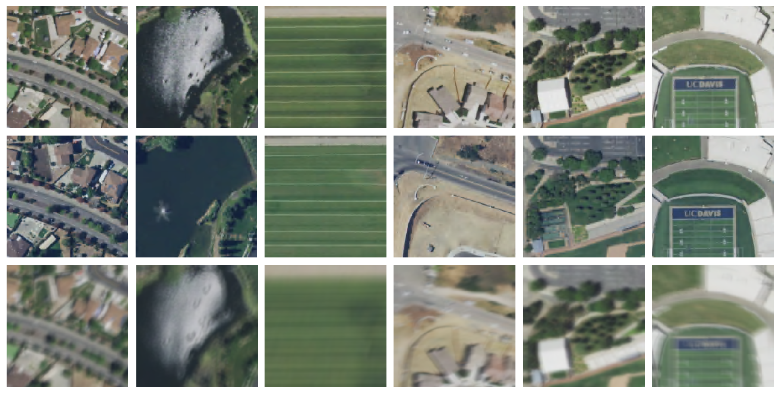
3.5. Datasets and Metrics

To the best of our knowledge, there are currently no publicly available datasets for remote sensing image deblurring with reference images. Therefore, we build a dataset for the reference-based deblurring algorithm in this work. The data are sourced from the United States Department of Agriculture (USDA), which takes remote sensing images of U.S. states every year. We select the remote sensing image of California captured in 2018 as the reference image and the image captured in 2020 as ground truth. The shape of the original image is 11,184 × 12,717 pixels. We have captured multiple areas from it, including farmland, vegetation and high-density urban areas. Furthermore, these regions are further cropped into a shape of $160\times 160$ pixels with overlapping. We take 82% of the dataset as the training set and 18% as the testing set. The training set contains 1138 pairs, while the testing set contains 240 pairs, where each pair consists of a clear image and a reference image.

Motion blur is a common type of image blurring in the field of remote sensing. It is mainly derived from the irregular movement of the imaging device during the exposure time. Zhang et al. [12] use linear motion kernels to create synthetically blurry images. To simulate more realistic and complex motion blur process, we use the random trajectory generation method proposed in the [16] to make motion blur kernels for generating our blurry images. The blur kernel size is $40\times 40$ in this work. Examples of our dataset are shown in Figure 6. However, our Ref-MFFDN does not make assumptions on blur type, and hence, may be extended to cases other than motion blur.

For quantitative evaluation of network performance, restored images are evaluated on the peak signal-to-noise ratio (PSNR) and structural similarity measure (SSIM) [34], which are widely used image quality evaluation metrics.

PSNR is an approximation to human perception of image reconstruction quality. Because of images’ wide dynamic range, PSNR is usually expressed as a logarithmic quantity using the decibel scale. Larger PSNR value usually means better reconstruction results. PSNR can be mathematically defined as:

$$PSNR(\mathit{I},\mathit{G})=20log\frac{max}{{\parallel \mathit{I}-\mathit{G}\parallel }_2}$$

(17)

where $ma{x}_I$ is the maximum possible pixel value of the image. When the pixels are represented using B bits per sample, $ma{x}_I=2^B-1$.

SSIM is a perception-based model which can measure the difference in structural information between two images. Here, we adopt SSIM to measure the difference between restored image and ground truth. Better restored results usually have larger SSIM value. SSIM can be mathematically defined as:

$$SSIM(\mathit{I},\mathit{G})=\frac{(2{\mu }_{\mathit{I}}{\mu }_{\mathit{G}}+C_1)(2{\sigma }_{\mathit{I}\mathit{G}}+C_2)}{({\mu }_{\mathit{I}}^2+{\mu }_{\mathit{G}}^2+C_1)({\sigma }_{\mathit{I}}^2+{\sigma }_{\mathit{G}}^2+C_2)}$$

(18)

where ${\mu }_{\mathit{I}}$ and ${\mu }_{\mathit{G}}$ represent the average of $\mathit{I}$ and $\mathit{G}$, respectively, while ${\sigma }_{\mathit{I}}$ and ${\sigma }_{\mathit{G}}$ represent the variance of $\mathit{I}$ and $\mathit{G}$, respectively. Parameter ${\sigma }_{\mathit{I}\mathit{G}}$ stands for the covariance of $\mathit{I}$ and $\mathit{G}$. $C_1$ and $C_2$ are two variables to stabilize the division with weak denominator, where $C_1={\left(k_{1}L\right)}^2$ and $C_2={\left(k_{2}L\right)}^2$. L is the dynamic range of the pixel-values, while $k_1=0.01$ and $k_2=0.03$ by default.

In addition, to evaluate the efficiency of our algorithm, the average inference time required to reconstruct latent sharp images is recorded.

3.6. Implementation Details

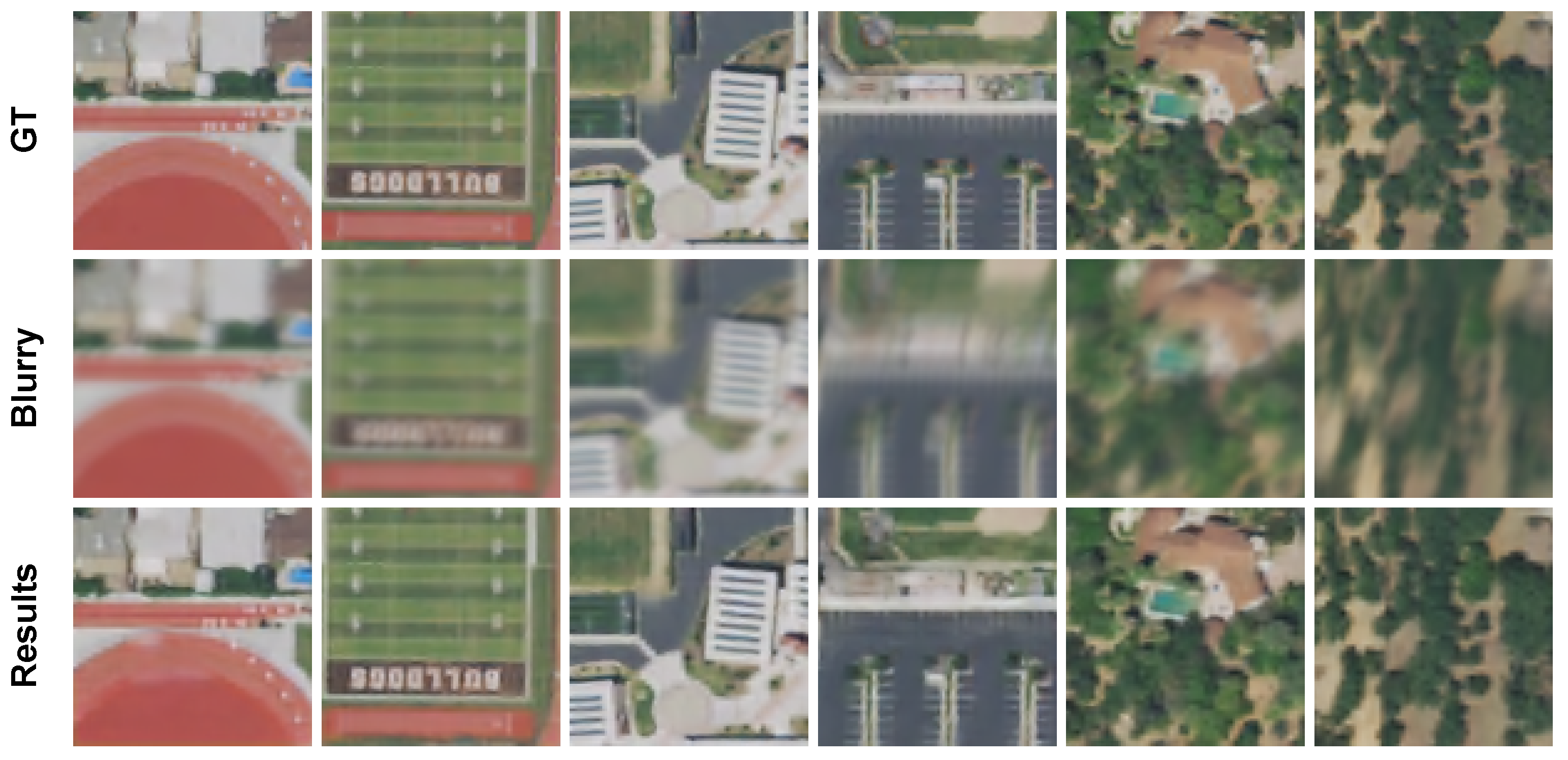
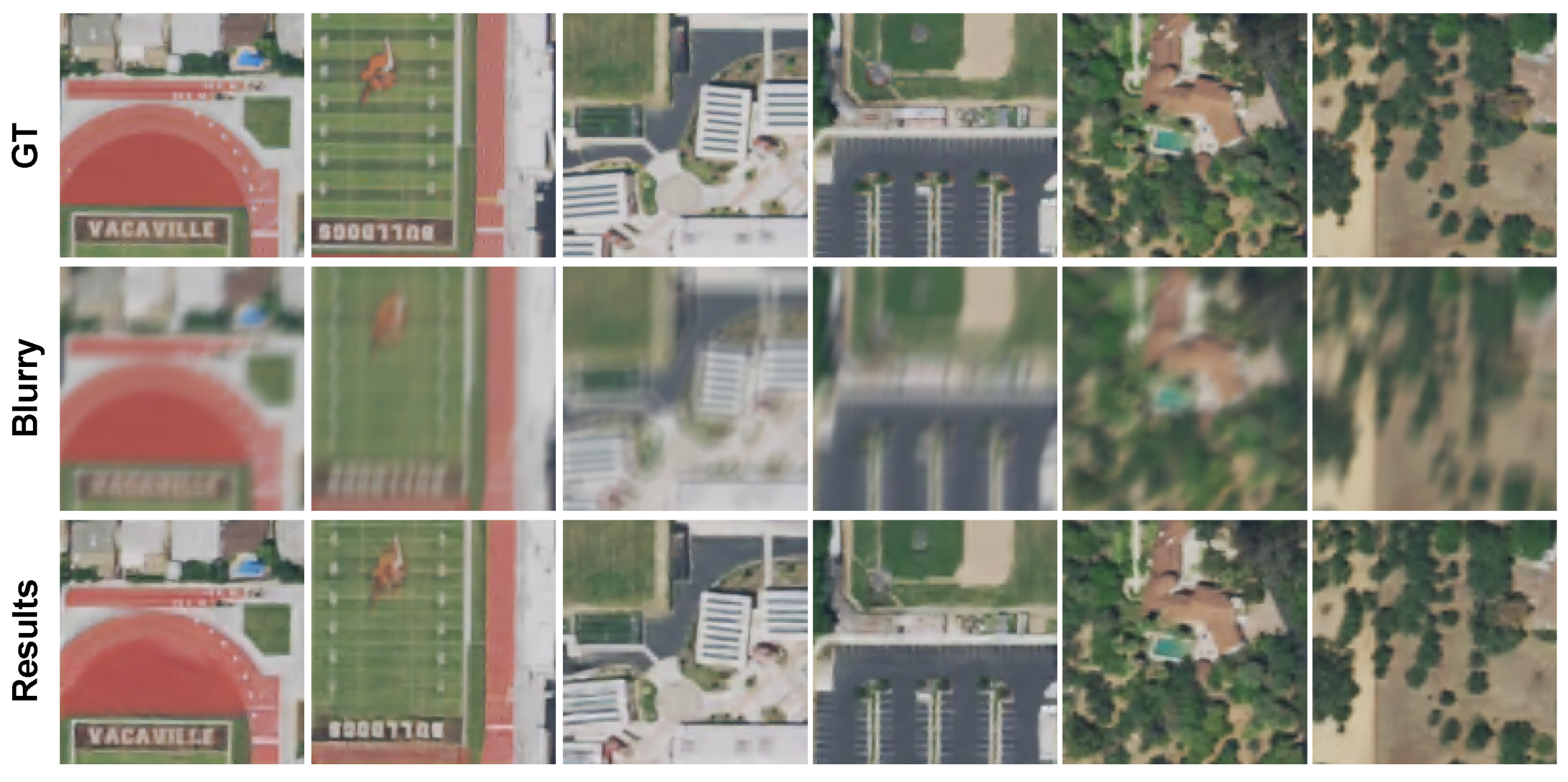
In our proposed method, the MFE contains three Resblocks with scale factor $\alpha =0.8$. Both EN and DN consist of 16 ResBlocks with scale factor $\alpha =0.8$. For the discriminator, we adopt the same structure used in TTSR [20]. We used as a training strategy that Ref-MFFDN is trained once while the discriminator is trained twice. The weight of ${\lambda }_{rec}$, ${\lambda }_{pec}$, ${\lambda }_{tpl}$ and ${\lambda }_{adv}$ are set to 1, $0.01$, $0.01$ and $0.001$, respectively. We adopt the Adam [35] optimizer with ${\beta }_1=0.9$, ${\beta }_2=0.999$. The learning rate is initialized as $2\times {10}^{-4}$ for EN and DN, while the learning rate of MFE is initialized as $1\times {10}^{-5}$ and the learning rate of discriminator is initialized as $1\times {10}^{-4}$.

During the training process, we take data augmentation operations by randomly cropping reference-blurry image pairs into image patches of $64\times 64$ pixels and randomly horizontally and vertically flipping followed by randomly rotating, where the flips and rotations on reference image and blurry image are independent. Then, we normalize the values of the training images to $[-1,1]$. The batch size is set to 16. We first warm up the network for 20 epochs where only ${\lambda }_{rec}$ is applied. Then, all losses are involved to train another 100 epochs. We implement our models with the PyTorch framework and train them on an NVIDIA RTX 2080Ti GPU.

Table 1. Software and hardware environment required for our experiments.

Hardware Environment	Single NVIDIA RTX 2080Ti GPU
	AMD 5800X
	Memory 3200 MHz, 32G
Software Environment	Torch 1.7.0 + cu110
	Torchvision 0.8.1 + cu110
	Numpy 1.21.2
	Python 3.8.5
	Visdom 0.1.8.9
	Opencv-python 4.4.0.44

shows the software environment and hardware environment required for our experiments in detail. The training takes 22 h to converge. The models are fully convolutional, and thus, can be applied to images of arbitrary size.

4. Results

To evaluate the performance of our proposed method, we compare our Ref-MFFDN with other SOTA deblurring methods, including PMP [11], DeepDeblur [15], DeblurGAN [16] and DeblurGAN-V2 [36]. For fair comparison, we follow the setting in [15,16,36] to train DeepDeblur, DeblurGAN and DeblurGAN-V2 on our proposed dataset. In Section 4.1, we test the performance of each algorithm on our proposed dataset. The robustness of Ref-MFFDN to input image size is discussed in Section 4.2.1. To verify the effectiveness of the MFFN module and the influence of MFE when added with different layers of ResBlocks, we conduct an ablation study in Section 4.2.

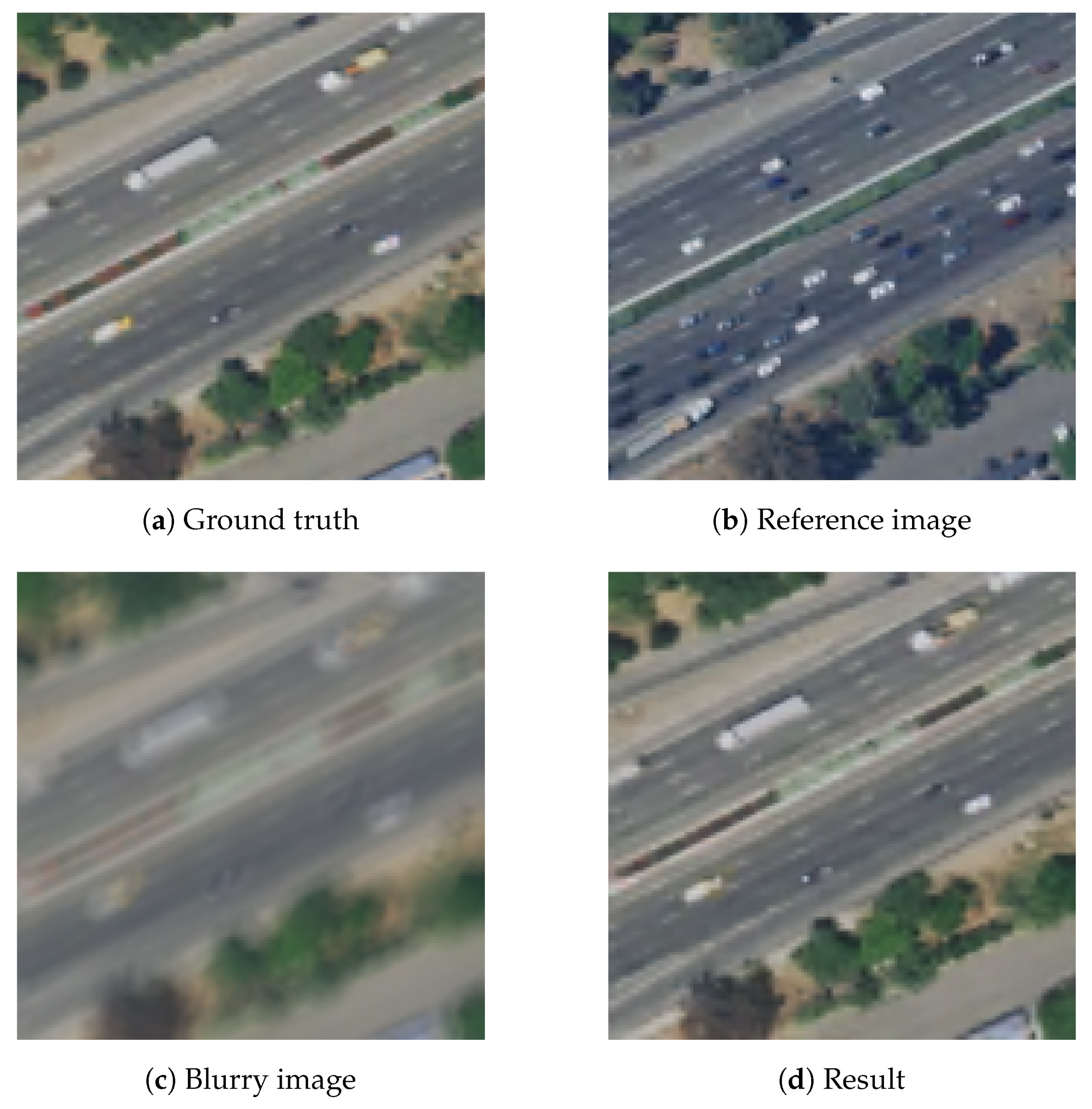
4.1. Quantitative and Qualitative Evaluation

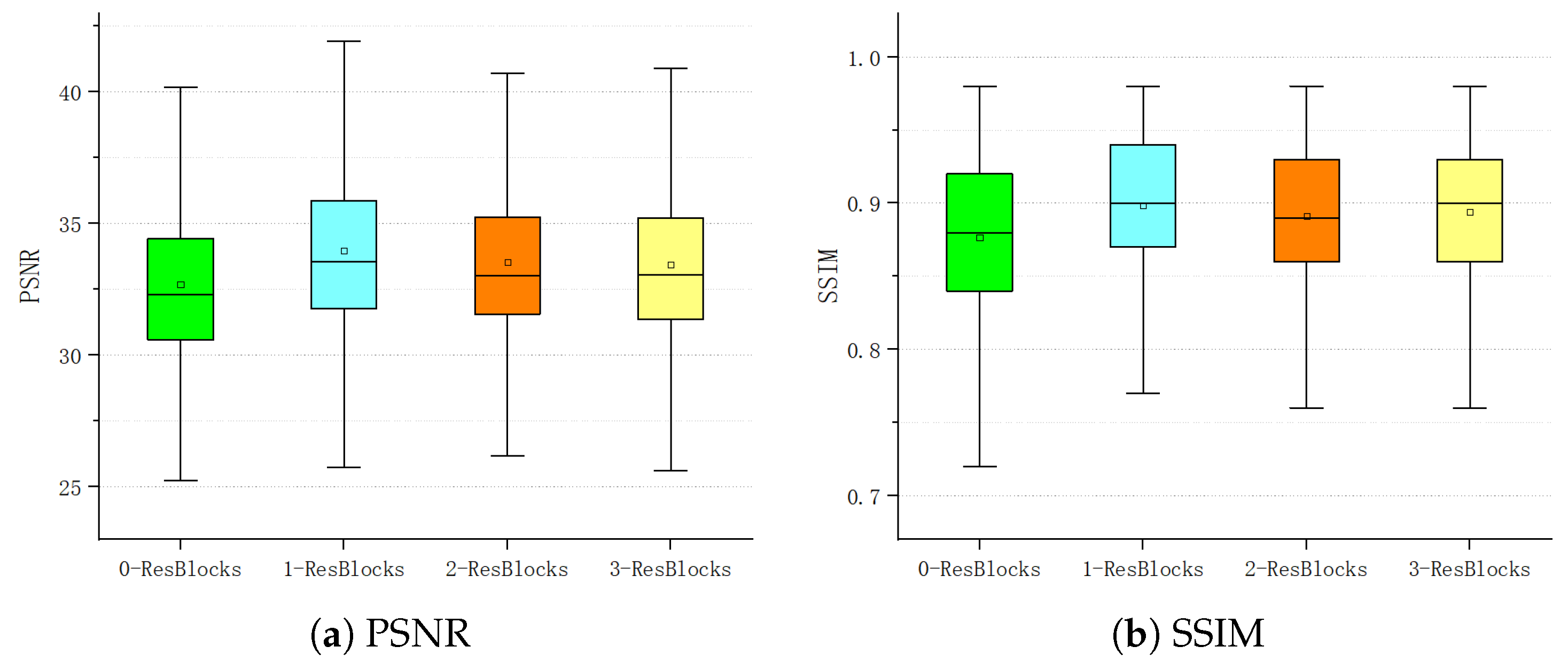
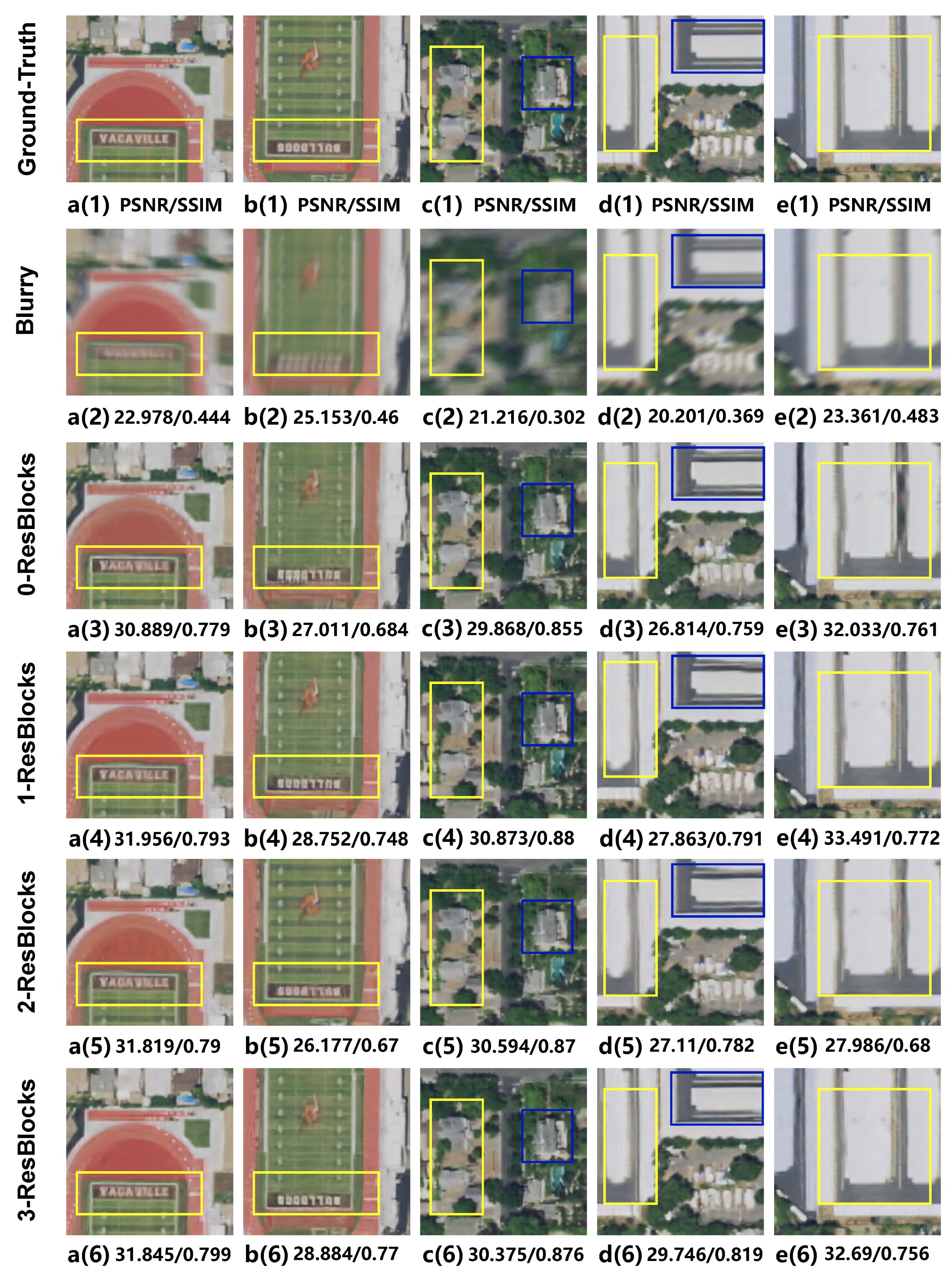
We quantitatively evaluated the restored images with $PSNR$ and $SSIM$ metrics. Moreover, we recorded the average inference time required for each algorithm to restore one latent sharp image. Since the PMP algorithm does not use GPU acceleration, all learning-based algorithms are run both on a CPU (AMD 5800X) and GPU to test inference speed for fairness.

Average PSNR, average SSIM and runtime of different deblurring methods are shown in

Table 2. Average PSNR, SSIM and Runtime of different deblurring methods. The highest score is highlighted in red while the second-highest score is highlighted in blue.

Methods	PSNR (dB)	SSIM	Runtime on CPU (s)	Runtime on GPU (s)
DeblurGAN [16]	27.627	0.710	0.33	0.10
DeblurGAN-V2 [36]	24.293	0.601	0.17	0.07
DeepDeblur [15]	32.549	0.875	0.50	0.15
PMP [11]	21.488	0.406	40.41	−
Ref-MFFDN	33.436	0.894	25.33	0.36

. As shown in this table, our method performs favorably against other deblurring methods on the average PSNR and average SSIM.

From the inference time of each algorithm on the CPU, DeblurGAN-V2 gets the highest score and DeblurGAN gets the second-highest score. The inference time used by our algorithm is about 149 times that of DeblurGAN-V2, 76 times that of DeblurGAN and 50 times that of DeepDeblur. However, our algorithm is still faster than iterative-based algorithms PMP. When running on GPU, the inference speed of our algorithm is greatly improved. Compared with other learning-based methods, the maximum time interval is reduced from more than 24 s to less than 0.3 s.

Figure 7 presents a statistical analysis of the PSNR and SSIM results of the comparison algorithms on the testing set. As shown in Figure 7a, the PSNR metric of images generated by our algorithm is higher than the comparison algorithm in the maximum, minimum, median, upper quartile and lower quartile. Figure 7b shows that images restored by Ref-MFFDN have the smallest value range on the SSIM metric compared to other deblurring algorithms, which demonstrates the robustness of Ref-MFFDN on our testing set.

A qualitative evaluation is presented in Figure 8. The latent sharp images restored by DeblurGAN have a good visual appearance but lack textures. Sometimes, DeblurGAN can even generate fake textures, e.g., Figure 8e(3). DeblurGAN-V2 can restore the clear latent sharp image, but the restored image has ghosting artifacts and fake textures as well. The images generated by DeepDeblur have a good visual appearance and rich texture information. However, when dealing with some fine textures, it is still insufficient, e.g., Figure 8a(5),b(5),d(5). PMP generate some ghost artifacts and fake textures on the examples, such as DeblurGAN-V2. In contrast, our proposed method can generate visually pleasing results with fine and realistic textures, whether for text, vegetation or buildings.

Furthermore, as shown in Figure 9, when the reference image is significantly different from the target image, the result restored by our algorithm are closer to the ground truth and do not have the redundant texture information of the reference image.

4.2. Ablation Study

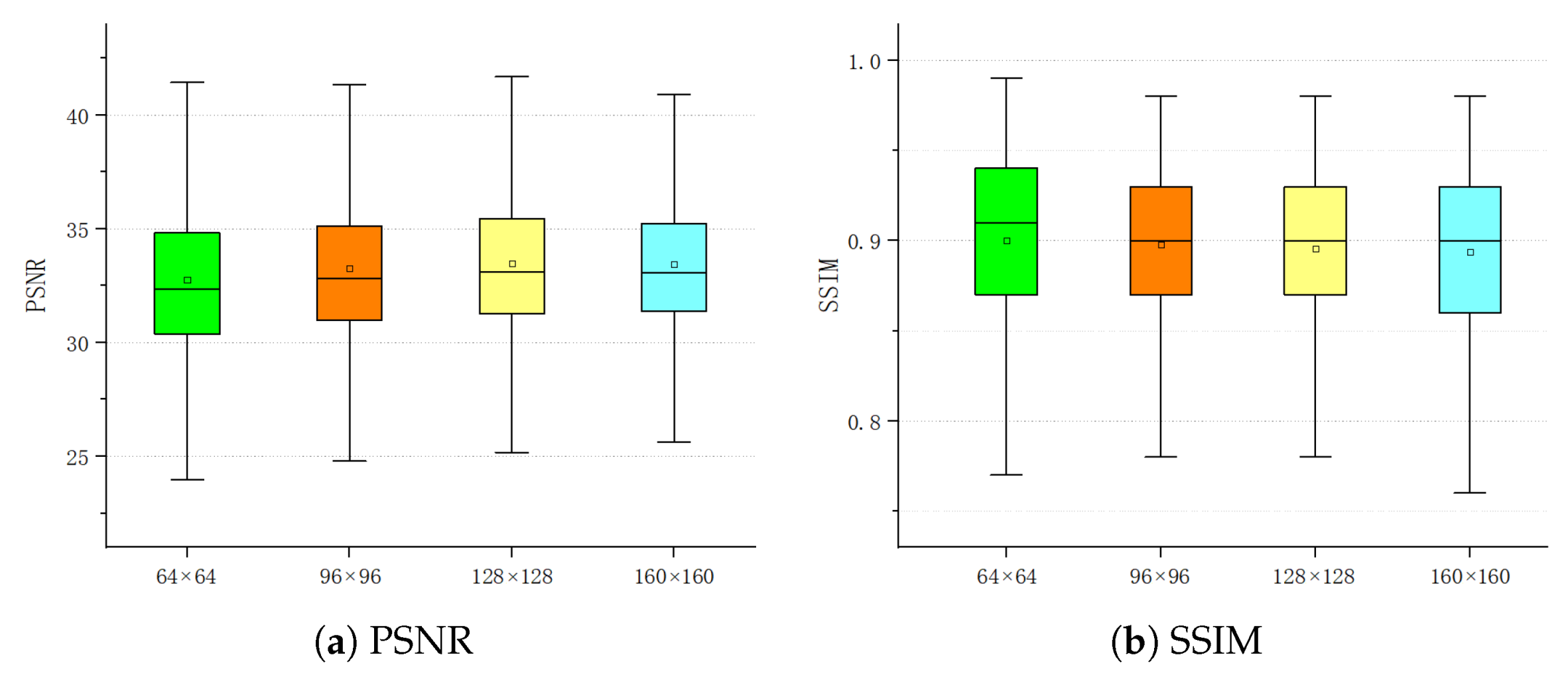
4.2.1. Robustness to Image Size

Ref-MFFDN is a fully convolutional network structure and the shape of the output image is consistent with the input image. To verify the robustness of our algorithm to the input image size, we conducted experiments with input images of size $64\times 64$, $96\times 96$, $128\times 128$ and $160\times 160$ pixels, respectively.

As shown in

Table 3. Average PSNR and SSIM of Ref-MFFDN when dealing with images of different scales. The highest score is highlighted in red while the second-highest score is highlighted in blue.

Image Shape	PSNR (dB)	SSIM
$64\times 64$	32.77	0.900
$96\times 96$	33.26	0.898
$128\times 128$	33.47	0.896
$160\times 160$	33.44	0.894

, images restored by Ref-MFFDN achieved close scores on average PSNR and SSIM metrics. Moreover, the PSNR and SSIM distributions on the testing set are also close as shown in Figure 10. The results quantitatively show that Ref-MFFDN is robust to the size of the input image.

Figure 11, Figure 12 and Figure 13 show the images restored by Ref-MFFDN when the input image size is $64\times 64$, $96\times 96$ and $128\times 128$ pixels, respectively. Ref-MFFDN works well on blurry images of different size as shown in Figure 11, Figure 12 and Figure 13. It qualitatively demonstrates the robustness of Ref-MFFDN to the size of the input image.

4.2.2. Effectiveness of MFFN and MFE

In this section, we retrain the network by removing the multi-level features fusion network (MFFN) with the same training strategy to verify the effectiveness of MFFN. Furthermore, we investigate the performance of the proposed method when we adopt a multi-level features extractor (MFE) with 0∼4 ResBlocks.

Multi-level features fusion network. As we can see from

Table 4. Average PSNR, SSIM and Runtime of our method with MFFN and without MFFN. The highest score is highlighted in red.

Methods	PSNR (dB)	SSIM	Runtime on CPU (s)	Runtime on GPU (s)
No MFFN	31.563	0.858	0.59	0.09
With MFFN	33.436	0.894	25.33	0.36

, when MFFN is added, the average PSNR performance can be improved from $31.563$ to $33.436$ and the average SSIM performance can be improved from $0.858$ to $0.894$, which verify the effectiveness of MFFN during the deblurring process. Correspondingly, inference time increased from 0.59 s to 25.33 s on CPU and increased from 0.09 s to 0.36 s on GPU after adding MFFN, which demonstrates that MFFN is the most time-consuming part of our algorithm.

The distribution of PSNR and SSIM metrics on the testing set of the above two structures are shown in Figure 14. Compared with structure using only EN and DN, the restored images by Ref-MFFDN can achieve overall higher PSNR and SSIM scores on the testing set.

As shown in Figure 15, guided by the reference image, the latent sharp images generated by Ref-MFFDN have more accurate textures and better visual perception. Comparing Figure 15a(3),f(3) with Figure 15a(4),f(4), the linear texture information on the building is better restored with the MFFN module. The ground texture in the yellow box is also better recovered when guided by the reference image, as shown in Figure 15c(4),d(4). Ref-MFFDN also shows better performance on vegetation textures, as shown in Figure 15b(4),e(4).

Multi-level features extractor.

Table 5. Average PSNR, SSIM and Runtime of Ref-MFFDN with different layers of ResBlocks added in MFE. The highest score is highlighted in red, while the second-highest score is highlighted in blue.

Methods	PSNR (dB)	SSIM	Runtime on CPU (s)	Runtime on GPU (s)
0-ResBlock	32.691	0.877	6.67	0.19
1-ResBlock	33.992	0.899	12.58	0.26
2-ResBlocks	33.545	0.891	19.00	0.32
3-ResBlocks	33.436	0.894	25.33	0.36

shows the quantitative evaluation results. Restored images acquired by Ref-MFFDN with 0-ResBlock MFE get the lowest scores on both the average PSNR metric and average SSIM metric, which demonstrates that adding the ResBlocks layer to MFE can effectively improve the quality of restored images. In other words, our network can better reconstruct latent sharp images guided by the high-level features of the reference images. When adding one to three layers of ResBlocks to the MFE, the restored images get close scores on the average PSNR and average SSIM metrics. In detail, the network with 1-ResBlock MFE achieved the highest scores in terms of average PSNR and average SSIM metrics, while the network with 2-ResBlocks MFE and the network with 3-ResBlocks MFE achieved the second-highest scores on average PSNR metric and average SSIM metric, respectively. For inference speed, each additional layer of ResBlock will increase the inference time by about 6 s on the CPU and about $0.6$ s on the GPU.

Figure 16 presents a statistical analysis on the PSNR and SSIM metrics of Ref-MFFDN when adding 0∼3 layers of ResBlocks to MFE. As shown in Figure 16a, the images restored by Ref-MFFDN with 1∼3 ResBlocks in MFE can achieve higher PSNR and SSIM metrics on maximum, minimum, mean, median, upper quartile and lower quartile than without ResBlocks in MFE.

Ref-MFFDN with 1-ResBlock MFE slightly outperforms the other two structures. Furthermore, the images reconstructed by the network have a smaller dynamic range on the PSNR metric when using 2-ResBlocks MFE and 3-ResBlocks MFE than when using 1-ResBlocks MFE. However, on the SSIM metric, this conclusion is just the opposite. As a result, it is difficult to quantitatively evaluate the performance of the above three structures.

Figure 17 shows the qualitative evaluation results. From this figure, we can observe that the image textures restored by Ref-MFFDN with 0-ResBlock MFE are insufficient, e.g., Figure 17a(3)–e(3). In contrast, images restored by Ref-MFFDN with ResBlocks in MFE show fine and detailed textures. In these experiments, the images restored by Ref-MFFDN adopting three layers of ResBlocks in MFE have the finest and most realistic textures. In more detail, the text textures in the yellow box of Figure 17a(6),b(6) are clearer than Figure 17a(3)–a(5),b(3)–b(5). Textures on building in Figure 17d(6)–e(6) are also more realistic than that in Figure 17d(3)–d(5),e(3)–e(5).

All in all, both quantitative and qualitative analyses demonstrate the effectiveness of adding ResBlocks to MFE. From the perspective of PSNR and SSIM metrics, Ref-MFFDN with 1-ResBlock MFE achieves the highest PSNR and SSIM scores. However, from the perspective of visual perception, images restored by Ref-MFFDN with 3-ResBlocks MFE, which fuses more advanced features of the reference image, are more visually pleasing.

5. Conclusions

In this paper, we propose a novel Reference-Based Multi-Level Features Fusion Deblurring Network (Ref-MFFDN) for Optical Remote Sensing Images, which transfers textures from the reference images to assist the restoration of latent sharp images. The proposed Ref-MFFDN consists of three modules: a multi-level features fusion network (MFFN), which extracts fused features from reference images and blurry images, an encoder network (EN), which extracts features from blurry images, and a decoder network (DN), which restores latent sharp images. Both quantitative and qualitative evaluations on the testing set demonstrate the effectiveness of the proposed method. However, as the key module for transferring reference image features to help reconstruct latent sharp images, MFFN increases the computational complexity of our algorithm. How to reduce inference time on the premise of ensuring algorithm performance will be the direction of our future research.

References

1. Kennedy, R.E.; Cohen, W.B.; Schroeder, T.A. Trajectory-based change detection for automated characterization of forest disturbance dynamics. Remote Sens. Environ. 2007, 110, 370–386. [Google Scholar] [CrossRef]
2. Netzband, M.; Stefanov, W.L.; Redman, C.L. Remote sensing as a tool for urban planning and sustainability. In Applied Remote Sensing for Urban Planning, Governance and Sustainability; Springer: Berlin/Heidelberg, Germany, 2007; pp. 1–23. [Google Scholar]
3. Wellmann, T.; Lausch, A.; Andersson, E.; Knapp, S.; Cortinovis, C.; Jache, J.; Scheuer, S.; Kremer, P.; Mascarenhas, A.; Kraemer, R.; et al. Remote sensing in urban planning: Contributions towards ecologically sound policies? Landsc. Urban Plan. 2020, 204, 103921. [Google Scholar] [CrossRef]
4. Mueller, N.; Lewis, A.; Roberts, D.; Ring, S.; Melrose, R.; Sixsmith, J.; Lymburner, L.; McIntyre, A.; Tan, P.; Curnow, S.; et al. Water observations from space: Mapping surface water from 25 years of Landsat imagery across Australia. Remote Sens. Environ. 2016, 174, 341–352. [Google Scholar] [CrossRef] [Green Version]
5. Fisher, A.; Flood, N.; Danaher, T. Comparing Landsat water index methods for automated water classification in eastern Australia. Remote Sens. Environ. 2016, 175, 167–182. [Google Scholar] [CrossRef]
6. Chan, T.F.; Wong, C.K. Total variation blind deconvolution. IEEE Trans. Image Process. 1998, 7, 370–375. [Google Scholar] [CrossRef] [PubMed] [Green Version]
7. Pan, J.; Hu, Z.; Su, Z.; Yang, M.H. Deblurring text images via L0-regularized intensity and gradient prior. In Proceedings of the IEEE Conference on Computer Vision and Pattern Recognition, Columbus, OH, USA, 23–28 June 2014; pp. 2901–2908. [Google Scholar]
8. Chen, L.; Fang, F.; Wang, T.; Zhang, G. Blind image deblurring with local maximum gradient prior. In Proceedings of the IEEE/CVF Conference on Computer Vision and Pattern Recognition, Long Beach, CA, USA, 15–20 June 2019; pp. 1742–1750. [Google Scholar]
9. Pan, J.; Sun, D.; Pfister, H.; Yang, M.H. Blind image deblurring using dark channel prior. In Proceedings of the IEEE Conference on Computer Vision and Pattern RECOGNITION, Las Vegas, NV, USA, 27–30 June 2016; pp. 1628–1636. [Google Scholar]
10. Wang, M.; Zhu, F.; Bai, Y. An improved image blind deblurring based on dark channel prior. Optoelectron. Lett. 2021, 17, 40–46. [Google Scholar] [CrossRef]
11. Wen, F.; Ying, R.; Liu, Y.; Liu, P.; Truong, T.K. A simple local minimal intensity prior and an improved algorithm for blind image deblurring. IEEE Trans. Circuits Syst. Video Technol. 2020, 31, 2923–2937. [Google Scholar] [CrossRef]
12. Zhang, Z.; Zheng, L.; Piao, Y.; Tao, S.; Xu, W.; Gao, T.; Wu, X. Blind Remote Sensing Image Deblurring Using Local Binary Pattern Prior. Remote Sens. 2022, 14, 1276. [Google Scholar] [CrossRef]
13. Bai, Y.; Jia, H.; Jiang, M.; Liu, X.; Xie, X.; Gao, W. Single-image blind deblurring using multi-scale latent structure prior. IEEE Trans. Circuits Syst. Video Technol. 2019, 30, 2033–2045. [Google Scholar] [CrossRef] [Green Version]
14. Sun, J.; Cao, W.; Xu, Z.; Ponce, J. Learning a convolutional neural network for non-uniform motion blur removal. In Proceedings of the IEEE Conference on Computer Vision and Pattern Recognition, Boston, MA, USA, 7–12 June 2015; pp. 769–777. [Google Scholar]
15. Nah, S.; Hyun Kim, T.; Mu Lee, K. Deep multi-scale convolutional neural network for dynamic scene deblurring. In Proceedings of the IEEE Conference on Computer Vision and Pattern Recognition, Honolulu, HI, USA, 21–26 July 2017; pp. 3883–3891. [Google Scholar]
16. Kupyn, O.; Budzan, V.; Mykhailych, M.; Mishkin, D.; Matas, J. Deblurgan: Blind motion deblurring using conditional adversarial networks. In Proceedings of the IEEE Conference on Computer Vision and Pattern Recognition, Salt Lake City, UT, USA, 18–23 June 2018; pp. 8183–8192. [Google Scholar]
17. Freeman, W.T.; Jones, T.R.; Pasztor, E.C. Example-based super-resolution. IEEE Comput. Graph. Appl. 2002, 22, 56–65. [Google Scholar] [CrossRef] [Green Version]
18. Timofte, R.; De Smet, V.; Van Gool, L. Anchored neighborhood regression for fast example-based super-resolution. In Proceedings of the IEEE International Conference on Computer Vision, Sydney, NSW, Australia, 1–8 December 2013; pp. 1920–1927. [Google Scholar]
19. Zhang, Z.; Wang, Z.; Lin, Z.; Qi, H. Image super-resolution by neural texture transfer. In Proceedings of the IEEE/CVF Conference on Computer Vision and Pattern Recognition, Long Beach, CA, USA, 15–20 June 2019; pp. 7982–7991. [Google Scholar]
20. Yang, F.; Yang, H.; Fu, J.; Lu, H.; Guo, B. Learning texture transformer network for image super-resolution. In Proceedings of the IEEE/CVF Conference on Computer Vision and Pattern Recognition, Seattle, WA, USA, 13–19 June 2020; pp. 5791–5800. [Google Scholar]
21. Dong, R.; Zhang, L.; Fu, H. Rrsgan: Reference-based super-resolution for remote sensing image. IEEE Trans. Geosci. Remote. Sens. 2021, 60, 1–17. [Google Scholar] [CrossRef]
22. Xu, X.; Pan, J.; Zhang, Y.J.; Yang, M.H. Motion blur kernel estimation via deep learning. IEEE Trans. Image Process. 2017, 27, 194–205. [Google Scholar] [CrossRef] [PubMed]
23. Zhang, J.; Pan, J.; Ren, J.; Song, Y.; Bao, L.; Lau, R.W.; Yang, M.H. Dynamic scene deblurring using spatially variant recurrent neural networks. In Proceedings of the IEEE Conference on Computer Vision and Pattern Recognition, Salt Lake City, UT, USA, 18–23 June 2018; pp. 2521–2529. [Google Scholar]
24. Li, Y.; Tofighi, M.; Geng, J.; Monga, V.; Eldar, Y.C. Efficient and interpretable deep blind image deblurring via algorithm unrolling. IEEE Trans. Comput. Imaging 2020, 6, 666–681. [Google Scholar] [CrossRef]
25. Suin, M.; Purohit, K.; Rajagopalan, A. Spatially-attentive patch-hierarchical network for adaptive motion deblurring. In Proceedings of the IEEE/CVF Conference on Computer Vision and Pattern Recognition, Seattle, WA, USA, 13–19 June 2020; pp. 3606–3615. [Google Scholar]
26. Yue, H.; Sun, X.; Yang, J.; Wu, F. Landmark image super-resolution by retrieving web images. IEEE Trans. Image Process. 2013, 22, 4865–4878. [Google Scholar] [PubMed]
27. Zheng, H.; Ji, M.; Wang, H.; Liu, Y.; Fang, L. Crossnet: An end-to-end reference-based super resolution network using cross-scale warping. In Proceedings of the European Conference on Computer Vision (ECCV), Munich, Germany, 8–14 September 2018; pp. 88–104. [Google Scholar]
28. Zheng, H.; Ji, M.; Han, L.; Xu, Z.; Wang, H.; Liu, Y.; Fang, L. Learning Cross-scale Correspondence and Patch-based Synthesis for Reference-based Super-Resolution. Proc. BMVC 2017, 1, 2. [Google Scholar]
29. Simonyan, K.; Zisserman, A. Very deep convolutional networks for large-scale image recognition. arXiv 2014, arXiv:1409.1556. [Google Scholar]
30. Gulrajani, I.; Ahmed, F.; Arjovsky, M.; Dumoulin, V.; Courville, A.C. Improved training of wasserstein gans. Adv. Neural Inf. Process. Syst. 2017, 30, 5769–5779. [Google Scholar]
31. Johnson, J.; Alahi, A.; Li, F.-F. Perceptual losses for real-time style transfer and super-resolution. In Proceedings of the European Conference on Computer Vision, Amsterdam, The Netherlands, 11–14 October 2016; Springer: Berlin/Heidelberg, Germany, 2016; pp. 694–711. [Google Scholar]
32. Ledig, C.; Theis, L.; Huszár, F.; Caballero, J.; Cunningham, A.; Acosta, A.; Aitken, A.; Tejani, A.; Totz, J.; Wang, Z.; et al. Photo-realistic single image super-resolution using a generative adversarial network. In Proceedings of the IEEE Conference on Computer Vision and Pattern Recognition, Honolulu, HI, USA, 21–26 July 2017; pp. 4681–4690. [Google Scholar]
33. Wang, X.; Yu, K.; Wu, S.; Gu, J.; Liu, Y.; Dong, C.; Qiao, Y.; Change Loy, C. Esrgan: Enhanced super-resolution generative adversarial networks. In Proceedings of the European Conference on Computer Vision (ECCV) Workshops, Munich, Germany, 8–14 September 2018. [Google Scholar]
34. Wang, Z.; Bovik, A.C.; Sheikh, H.R.; Simoncelli, E.P. Image quality assessment: From error visibility to structural similarity. IEEE Trans. Image Process. 2004, 13, 600–612. [Google Scholar] [CrossRef] [PubMed] [Green Version]
35. Kingma, D.P.; Ba, J. Adam: A method for stochastic optimization. arXiv 2014, arXiv:1412.6980. [Google Scholar]
36. Kupyn, O.; Martyniuk, T.; Wu, J.; Wang, Z. Deblurgan-v2: Deblurring (orders-of-magnitude) faster and better. In Proceedings of the IEEE/CVF International Conference on Computer Vision, Seoul, Korea, 27 October–2 November 2019; pp. 8878–8887. [Google Scholar]
Figure 1. The overall architecture of Ref-MFFDN.
Remotesensing 14 02520 g001
Figure 2. The structure of the multi-level features extractor.
Remotesensing 14 02520 g002
Figure 3. The process of feature fusion.
Remotesensing 14 02520 g003
Figure 4. The structure of the encoder network.
Remotesensing 14 02520 g004
Figure 5. The structure of the decoder network.
Remotesensing 14 02520 g005
Figure 6. Examples of our proposed dataset. (Top row): ground truth. (Second row): reference image. (Bottom row): blurry image.
Remotesensing 14 02520 g006
Figure 7. The distribution of PSNR and SSIM of different deblurring methods on the testing set. The box plot displays the maximum, upper quartile, median, lower quartile, and minimum of results from top to bottom. The rectangle inside the box represents the average metrics of results.
Remotesensing 14 02520 g007
Figure 8. Visual comparison of images restored by different deblurring methods on the testing set.
Remotesensing 14 02520 g008
Figure 9. Algorithmic restoration result when there are extra textures in the reference image.
Remotesensing 14 02520 g009
Figure 10. The distribution of PSNR and SSIM of Ref-MFFDN when dealing with input images at different scales. The box plot displays the maximum, upper quartile, median, lower quartile, and minimum of results from top to bottom. The rectangle inside the box represents the average metrics of results.
Remotesensing 14 02520 g010
Figure 11. The images restored by Ref-MFFDN of size 64 × 64 pixels.
Remotesensing 14 02520 g011
Figure 12. The images restored by Ref-MFFDN of size 96 × 96 pixels.
Remotesensing 14 02520 g012
Figure 13. The images restored by Ref-MFFDN of size 128 × 128 pixels.
Remotesensing 14 02520 g013
Figure 14. The distribution of PSNR and SSIM of our method with MFFN and without MFFN on the testing set.
Remotesensing 14 02520 g014
Figure 15. Visual comparison of images restored by our method with MFFN and without MFFN.
Remotesensing 14 02520 g015
Figure 16. The distribution of PSNR and SSIM of Ref-MFFDN with different layers of ResBlocks added in MFE on the testing set. The box plot displays the maximum, upper quartile, median, lower quartile, and minimum of results from top to bottom. The rectangle inside the box represents the average metrics of the results.
Remotesensing 14 02520 g016
Figure 17. Visual comparison of images restored by Ref-MFFDN with different layers of ResBlocks added in MFE.
Remotesensing 14 02520 g017