Automatic Calibration of a LiDAR–Camera System Based on Instance Segmentation

Abstract

In this article, we propose a method for automatic calibration of a LiDAR–camera system, which can be used in autonomous cars. This approach does not require any calibration pattern, as calibration is only based on real traffic scenes observed by sensors; the results of camera image segmentation are compared with scanning LiDAR depth data. The proposed algorithm superimposes the edges of objects segmented by the Mask-RCNN network with depth discontinuities. The method can run in the background during driving, and it can automatically detect decalibration and correct corresponding rotation matrices in an online and near real-time mode. Experiments on the KITTI dataset demonstrated that, for input data of moderate quality, the algorithm could calculate and correct rotation matrices with an average accuracy of 0.23°.

1. Introduction

Apart from GPS/INS, LiDAR and cameras are the basic types of sensors used in autonomous cars. In the current systems, their calibration requires a calibration pattern and this should be done before autonomous driving. However, during operation, a small rotation of a sensor can remain unnoticed, and even rotation by a fraction of degree affects data quality until the next calibration. Automatic calibration can be of particular importance during data collection, as changes of sensor parameters with time may render the logged data worthless. In practical applications, calibration is usually performed at the beginning of the data collection campaign, with further sensor calibration possible after several weeks (which means after the car has driven thousands of kilometers).

Currently, calibration of the sensors of autonomous vehicles is performed manually and off-line, based on the calibration pattern. In the literature, there is some research reported whereby extrinsic calibration of a LiDAR-camera system can be done on-line, but this requires specific calibration objects, which must appear in the image. For example, in [1,2], a chessboard was used; in [3,4], calibration was based on planar patterns with circles; and in [5], triangle or diamond-shaped boards were used. There are also methods where calibration is based on spatial objects in the field of view, for example trihedrons [6,7,8] or spheres [9]. Moreover, several methods were proposed for LiDAR–camera system calibration that do not require any calibration pattern. For example, the approach described in [10] exploits the natural scenes observed by both sensors, and the matching of data from both sensors is based on maximizing the correlation between the laser reflectivity and the camera intensity. The shortcoming of this approach is that, apart from depth information, it requires reflectivity data from LiDAR. Another method, presented in [11], is based on sensor fusion odometry and requires a specific rotational motion of the sensors in the horizontal and vertical directions.

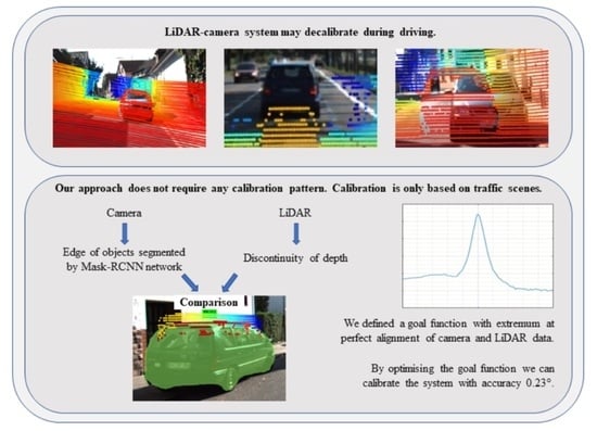
Our approach is only based on the camera image and depth data from LiDAR, without using any additional information. Automatic calibration of a LiDAR–camera system can be performed on-line, during vehicle driving. In contrast to existing methods, our method is based on semantic segmentation of objects that appear in real traffic scenes. The borders of objects segmented in the camera image are superimposed with discontinuities of depth on LiDAR data. This approach recently became feasible, when the quality of automatic pixel-wise semantic segmentation rose to a sufficient level, as the result of deep neural network development. This method can detect situations where the current calibration parameters, particularly yaw, pitch, and roll angles, do not ensure the proper alignment of data, and it automatically corrects corresponding rotation matrices during driving, in near real-time.

This paper is organized as follows: in Section 2 we describe the state of the art of object segmentation, which is crucial for our algorithm. We discuss features of Detectron2, which we used for the segmentation of cars, and we review the literature on using depth information for facilitating segmentation. Section 3 is related to our input data, taken from the KITTI dataset. In Section 4, we present the concept of our method, and in Section 5 preliminary experiments, which allowed us to set the parameters of the goal function and to adjust the optimization procedure, to properties of the goal function. In Section 6, we describe details of the algorithm and present the results. Finally, Section 7 contains our conclusions and plans for future work.

2. Segmentation

Segmentation is an important part of image analysis and one of the most difficult problems in computer vision. The results of classical segmentation methods, based on properties of image sub-areas such as color or texture, often are inconsistent with the semantics of the image. However, recent deep convolutional neural networks, apart from the classification of image objects, can yield a relatively high quality semantic segmentation of an image. For an exhaustive survey on image segmentation using deep convolutional networks, see [12]. One of the most popular architectures of this type is Mask RCNN, proposed in 2017 [13], and included in the Detectron2 [14] network system. The architecture of Mask RCNN, similarly to Faster RCNN [15], is based on a region proposal network (RPN); a subnetwork which indicates regions that potentially may contain an object. It has, however, one more output, and apart from the class labels and bounding boxes, it returns the object masks. In our method, we used the pretrained Mask R-CNN model, based on a ResNet+FPN backbone (mask_rcnn_R_50_FPN_3x). We chose this model because, according to the literature, it is currently the most effective network that, besides object detection, provides high quality pixel-wise segmentation, while most other detectors, such as YOLO or classical Faster-RCNN, only retune the bounding boxes of detected objects. It is, however, worth noting that for detection tasks, where pixel-wise segmentation is not required, the highest performance in road object detection is achieved by the YOLOv4 architecture [16]. Moreover, Detectron2 is available along with a set of weights trained for detection of relevant objects that appear in traffic scenes, such as vehicles or pedestrians. This is particularly important, because convolutional networks with an instance segmentation capability require pixel-wise segmentation of training data, so preparation of a database for training is much more difficult than for networks that merely return bounding boxes of the detected objects. Segmentation in the deep network is performed in parallel with detection and classification of objects; thus, it is based on the borders of semantic objects, rather than on local differences of image features. The output, apart from the boundaries of objects, contains their classification. The reliability of segmentation using Detectron2 is very high compared to the classical methods, which are imperfect because they are not based on the semantic meaning of the image. By classical methods, we mean approaches based on color, texture, and phase features, which are used as the input for such techniques as region-growing and split and merge, or to more complex algorithms, such as iterative propagation of edge flow vector fields [17] or methods based on random Markov fields [18]. On the other hand, it is worth mentioning that methods based on deep learning return rough borders of objects, and that their accuracy of localization of object boundaries is generally lower than in the case of classical segmentation methods, where the edge is detected at the location that separates two image areas with different properties.

If depth information is available, it can be used to solve or to improve segmentation; for example, by using depth as an additional input to the network. In [19], Mask RCNN was modified by adding an additional pipeline for depth image processing, and feature maps from RGB and from depth images were concatenated at a certain stage. The results were marginally better than for Mask RCNN, based on a RGB image. In [20], the depth image was triplicated, to adjust it to the architecture of Mask RCNN, which accepts a three-channel input. Segmentation based on this approach outperformed existing point cloud clustering methods. Several networks that operate on 3D images have been developed. Examples of such networks include VoxelNet [21], YOLO 3D [22], and point pillars [23]. There are also simple algorithms where depth discontinuity is used to detect the border between the foreground object and the background [24]. For some specific applications, when the distance range to the object and to the background do not overlap, easy methods based on depth histogram thresholding are sufficient; as for example in [24], where this approach was successfully used to segment the car driver from the background. However, the method failed to segment a standing person, since in the bottom part of the object, the distance to the background and to the foreground object overlapped. In our method, however, depth information is not used for segmentation, but for verification of whether a depth image from LiDAR is precisely superimposed with the camera image. We can, therefore, only use a part of the object, for example the upper part of the car, where the background is far behind the object.

3. Input Data

In our experiments we used the KITTI (Karlsruhe Institute of Technology and Toyota Technological Institute) dataset [25], which contains data from a Velodyne HDL-64E rotating 3D laser scanner and four PointGray Flea2 cameras (two color and two grayscale cameras). Sensors were calibrated and synchronized (timestamps are available). Intrinsic and extrinsic camera calibration was performed based on chessboard calibration patterns, and Velodyne was calibrated with respect to the reference camera, by minimizing disparity error using Metropolis–Hastings sampling [1]. Calibration includes both rotation and translation, so that data from all sensors are transformed to the common coordinate system. Data from the inertial and GPS navigation systems are also included; but in this article, we focused on the detection of objects observed by LiDAR and cameras, so we did not use any location data. LiDAR parameters and the quality of output data are rather low compared to more recent datasets such as nuScenes [26]. Velodyne HDL-64E contains 64 rotating lasers, data are taken with a horizontal resolution of 0.08° and vertical resolution of 0.4°. However, we will demonstrate that we can match the LiDAR output with camera images with a relatively high accuracy, by using statistical data from many frames. The resolution of the cameras is 1392 × 512. For this study, we used all 7481 images from the “3D Object Detection Evaluation 2017” dataset included in the KITTI Vision Benchmark Suite, as well as the corresponding Lidar point clouds.

In order to more closely examine the quality of LiDAR data, we developed a piece of software that presents LiDAR points together with car masks returned by the Detectron network. LiDAR points are shown only in the vicinity of the upper edge of car masks. They are presented in the form of triangles, which point up (▲) if they are located below the edge of the detected mask (so they are in the mask area), or down (▼) if they are located above the mask edge; see Figure 1. The color represents the distance, with the scale adjusted for each object separately. The most distant pixels are blue and the closest are red. Browsing the KITTI dataset, we can see that the LiDAR data are imperfect.

In Figure 1, depth is measured correctly, and in the top image the LiDAR data seem correct. However, in a close-up of the bottom image, we can see that near the object, border points are reported as a close (object points) and far (background points) interlace. This can be attributed to the inaccuracy of beam directions from neighboring lasers in the LiDAR. The result is that a beam from a higher laser hits the lower points of the image, but its location is assigned on the basis of the assumed (and not actual) direction of the beam.

In some scenes, the distance to some objects is incorrectly measured, as in the example in Figure 2. This can be attributed to the limitations of the Velodyne range and to reflections of the light.

Therefore, the proposed method must be robust to these types of error. We will achieve this with operation on a number of recent frames, so that errors from single frames will compensate.

4. Outline of the Method

Our method is based on the fact that, if the parameters that describe mutual position and orientation of the camera and LiDAR are precisely estimated, the distance of LiDAR points that are located within the object mask detected by Detectron (from the camera image) should be smaller than for LiDAR points located in the vicinity, but in the background, outside the mask area. As already noted, the depth difference between the object and the background is large in the neighborhood of the upper part of the object, while in the bottom part, where an object touches the ground, the object border may not coincide with the depth discontinuity. This is why, in typical scenes, a depth map can be used for simple and faultless segmentation, but only of the upper part of objects [24]. Our method is based on the comparison of image depth in the upper part of the object mask and in the zone directly above the mask. Detectron2 has been trained for detection of vehicles, pedestrians, and bicycles. In our method only vehicles are used, because they are the most common in traffic scenes, their segmentation is almost faultless and the upper part of the mask is wide and smooth. The details on how these two zones are calculated from the mask returned by Detectron2 are presented in Figure 3. For the calculation of zones, two parameters are used: η—relative width of the vertical range margins (in relation to the width of the object), and ε—relative horizontal range of zones (in relation to the height of the object). In the algorithm, η = 0.1 and ε = 0.15.

Masks are calculated from the camera image, and depth is based on LiDAR data, so correct calibration of the LiDAR–camera system should ensure the maximum difference between the average distance of points above and below the upper edge of object masks. If any inaccuracy of calibration appears, perhaps resulting from a physical movement of the LiDAR or camera, this will result in a decrease of this difference. By maximizing this difference over the calibration parameters, it is possible to correct the calibration matrix in the event of an undesired rotation of the camera or LiDAR.

Automatic calibration of the LiDAR–camera system cannot be based on a single traffic scene, and it is necessary to take into consideration a series of frames. There are several reasons for this:

• Many LiDAR points have incorrect depth values, and location data of LiDAR points are inaccurate (see Figure 1)
• Object masks calculated by Detectron are usually relatively exact, but for some object instances the accuracy is insufficient for automatic calibration
• Some frames do not contain relevant objects, or they only contain small objects, insufficient for optimization
• Our method is based on an assumption that the distance to the car is smaller than to the background above the car, which is generally true; although there are exceptions, for example, when the top part of the car is obstructed by a tree branch

We optimize the goal function F, defined in the next part of this chapter, over rotation of LiDAR in all possible directions, but we do not include a correction of translation. The reason is that, even small, unnoticeable rotation of the sensor, e.g., by one or two degrees, results in a loss of calibration. For example, the pitch displacement in Figure 4b is only 3° and alignment of images is completely lost. Such rotation may result from external force, deformation of mounting, etc. In contrast, unintended translation of the sensor is practically impossible, due to the way the sensors are mounted. Moreover, unnoticeable translation of sensor, even by several millimeters, in practice does not affect the alignment of images of distant objects. Moreover, our procedure does not include calibration of intrinsic camera parameters, which do not change suddenly by large values, and we assume that they are calibrated off-line, using standard procedures.

The goal function F is defined as the mean value over relevant objects (i.e., objects that meet conditions of inclusion in the goal function) of the differences between average distance to the object in the zone above the mask upper edge and the average distance to the object in the zone below the mask upper edge:

$$F({\alpha }_r,{\alpha }_p,{\alpha }_w)=\underset{ob\in I}{mean}\left(\underset{a\in A(ob)}{mean}d(a)-\underset{b\in B(ob)}{mean}d(b)\right)$$

(1)

where

• α_r, α_p, α_w—roll, pitch, and yaw of LiDAR rotation (see Figure 4).
• I—the set of frames taken into consideration for calculations
• ob—the set of relevant objects, i.e., objects identified as cars, which meet conditions of inclusion in the goal function
• A—the set of LiDAR points located in the zone above the object mask upper edge. A is defined for each object and depends on the rotation of the image, so A = A(ob, α_r, α_p, α_w)
• B—the set of LiDAR points located in the zone below the object mask upper edge. B is defined for each object and depends on the rotation of the image, so B = B(ob, α_r, α_p, α_w)
• D—distance to a LiDAR point

Conditions of object inclusion in the goal function include:

• The number of LiDAR points in sets A and B must exceed the threshold (at least five points in each zone are required)
• The average distance of LiDAR points must be in a specified range (in our case, between 5 m and 100 m). This ensures that the size of vehicles in the camera image is the most suitable for automatic semantic segmentation.

We expect a maximum value of the goal function F when LiDAR data are correctly aligned with the camera image.

5. Preliminary Experiments

The goal of the experiments presented in this section was to examine the properties of the goal function; whether is it continuous, differentiable, does it have many local extrema, etc. These properties are relevant for the choice of optimization algorithm and optimization parameters, especially how many frames should be taken into consideration for the goal function calculation.

5.1. Properties of the Goal Function

In the first series of experiments, we examined how the goal function depends on loss of calibration of the LiDAR–camera system, separately for roll, pitch, and yaw (see Figure 4). The properties of the goal function are important for the choice of optimization procedure.

From the point of view of the optimization algorithms, it is important to note that F is not differentiable and, moreover, not continuous as a function of roll, pitch, and yaw. It is a multidimensional step function (piecewise constant function), which changes value when, as a result of rotation, at least one LiDAR point changes its membership of the sets A(ob) and B(ob) of any object ob in the set I.

To confirm this, we plotted F(0, 0, α_w) for different ranges of yaw. In Figure 5a, yaw varies from −5° to 5°. Only 10 frames were taken into consideration for the calculation; thus, fluctuations are very strong, but no staircase property can be observed because, when rotating in this range, many LiDAR points change membership to A and B. In Figure 5b, function F is presented with a 100-times zoom (for the range −0.05° to 0.05°). Figure 5c shows a 10,000-times zoom (range from −0.0005° to 0.0005°), and here the step character of F is noticeable.

In the next experiments, we examined the behavior of F in the whole range of angles of roll, pitch, and yaw, from −180° to 180°. In Figure 6, we present the intersection of F when one of these three angles varies and other two are set to 0. As expected, if the absolute value of pitch is too high, F is undefined. This is because the cloud of LiDAR points is shifted out of the area where the objects appear. In contrast, F is defined in the whole range of yaw, from −180° to 180°, because LiDAR data are provided for the whole environment around the car. Similarly, F is defined in the whole range of roll because the LiDAR cloud, even rotated upside down, stays in the camera field of view.

The conclusion from the above experiments was that, when optimizing F, the optimization method must be appropriate for non-continuous functions, with many local extrema and fluctuations of value. The function domain is limited, so the search area should be constrained. For the experiments, we chose a pattern search algorithm. This method is based on comparing the values of the goal function at the grid nodes. When a point with a lower value of the goal function is found, compared to the current point, it becomes the new current point and the grid size is doubled, otherwise it is halved. This method is appropriate for constrained optimization of non-continuous functions. For details of the pattern search algorithm see [27]. Technically, the optimization procedure is looking for the global minimum, so we maximize F by minimizing −F.

5.2. Influence of the Number of Frames on the Goal Function Shape

The shape of the goal function is crucial to the difficulty of optimization, especially because our goal function F contains fluctuations similar to noise (see Figure 6), caused by the discrete number of LiDAR points that fall into zones above and below the mask upper edge, presented in Figure 3 (see Section 5.1 and Figure 5 for more detailed explanation and illustration). In Figure 7, we present how the goal function F depends on roll (Figure 7a), pitch (Figure 7b), and yaw (Figure 7c), when the other two angles are set to zero. We created separate charts for roll, pitch, and yaw, because the behavior of F is slightly different for each of these angles:

• F as a function of pitch F(0, α_p, 0) has relatively small fluctuations. This is because non-zero roll causes a direct shift of some LiDAR points, from the zone above the mask upper edge, to the zone below (see Figure 3), or vice versa.
• Fluctuations of F are the most visible for the variable yaw, i.e., in chart of F(0, 0, α_w). The reason is that the upper part of the car mask is usually horizontal rather than vertical, so the background LiDAR points in the zone above the mask upper edge are only replaced by other background points, and the foreground points in the zone below the mask upper edge are replaced by background points much more slowly than in the case of pitch, because the horizontal range of this zone is much higher than the vertical range. Thus, a small LiDAR yaw has a small influence on mean d(a) and mean d(b) in (1).
• Fluctuations of F(α_r, 0, 0) have an intermediate magnitude compared to F(0, α_p, 0) and F(0, 0, α_w). The influence of roll on F depends on where the object is located: for objects located at the sides of the image, roll has an influence on F similar to pitch; while for objects in the center, the influence can be different for different parts of the object (similar to positive pitch on the left and to negative pitch on the right).

The most important part of this experiment was exploring how F depends on the number of frames used for calculating the mean value in Equation (1). As we can see in Figure 7, for a small number of frames, F has strong fluctuations, so optimization is difficult, and moreover location of the goal function global extremum can be accidental. On the other hand, considering too many frames increases the delay of automatic calibration. Based on the charts, we could say that using fewer than 50 frames could lead to random results.

5.3. Local Extrema Avoidance

In order to verify the ability of the optimization procedure to find the global maximum of F, we simulated 100 cases of decalibration. For each decalibration, we ran the pattern search algorithm S times (in this experiment S = 10), each time from a different starting point, in order to avoid falling into a local optimum. Starting roll, pitch, and yaw were chosen randomly, between −5° and 5° from uniform distribution. Let ε be the Euclidean distance between the minimum found by the algorithm and the point corresponding to the actual value of decalibration:

$$\epsilon =\sqrt{{\left({\alpha }_r-\overline{{\alpha }_r}\right)}^2+{\left({\alpha }_p-\overline{{\alpha }_p}\right)}^2+{\left({\alpha }_w-\overline{{\alpha }_w}\right)}^2}$$

(2)

where α_r, α_p, and α_w are simulated LiDAR raw, pitch, and yaw, and $\overline{{\alpha }_r}$, $\overline{{\alpha }_p}$, and $\overline{{\alpha }_w}$ are the corresponding values of raw, pitch, and yaw calculated by our method. The goal function is very irregular, with a large number of local minima close to the global one. Therefore, we accept certain error, and when the distance ε given by (2) is below a threshold th = 1, we assume that the global minimum was found successfully. We performed the optimization 100 times, each time for different LiDAR decalibration, and the global minimum was found in 47% of optimizations when the goal function was calculated from the 50 most recent frames, and in 59% of optimizations when the goal function was calculated from the 100 most recent frames. We could, therefore, roughly estimate the probability p of falling into a local extremum in a single optimization, which is 0.53 and 0.41, respectively. In Figure 8 we present a histogram of distances ε for this experiment, the value for each bin represents the number of optimizations, where the distance ε given by (2) falls into the bin.

If we perform a series of optimizations of the same goal function F (calculated from the same set of frames), consecutive optimizations are independent. The result of a single optimization only depends on the starting point, which we chose randomly from a uniform distribution. Consequently, the probability of missing the global extremum every time in a series of k optimizations is p^k, where p is the probability of falling into a local extremum in a single optimization.

6. Automatic Calibration; Algorithm Details and Results

In this section we describe the experiments that simulated the loss of calibration of a LiDAR–camera system while a car is in motion. We verify the ability of the algorithm to detect and automatically correct LiDAR angular displacement based on images captured during driving. We carried out 10 experiments. In each, we simulated accidental rotation of LiDAR by introducing additional yaw, pitch, and roll to the calibration matrices, and for each experiment, F was optimized 10 times with a pattern search algorithm from different staring points, using the 50 most recent frames. The probability of falling into a local extremum is 0.53, so the risk of missing the global extremum in all 10 optimizations is 0.0017 (0.53 to the power of 10). In

Table 1. Simulation of 10 decalibration experiments during car movement. Each row of the table corresponds to one experiment: F was optimized using the 50 most recent frames (different for each decalibration); 10 times, from 10 starting points.

Actual Decalibration			Calculated Correction			Errors			Distance	F
Roll	Pitch	Yaw	Roll	Pitch	Yaw	Roll	Pitch	Yaw
3.011	−2.004	2.756	−2.647	2.045	−2.823	0.364	0.041	−0.067	0.37	−8.827
−3.859	0.408	−0.836	3.847	−0.410	0.685	−0.013	−0.001	−0.150	0.15	−7.838
0.891	−0.203	−3.013	−0.731	0.246	2.911	0.160	0.044	−0.103	0.20	−8.084
0.163	2.070	3.136	0.564	−1.926	−3.090	0.727	0.145	0.046	0.74	−7.586
−3.080	2.770	3.645	3.436	−2.476	−3.749	0.356	0.293	−0.104	0.47	−8.271
2.646	−2.563	1.821	−2.371	2.548	−1.930	0.275	−0.015	−0.109	0.30	−8.244
−3.902	3.321	4.716	4.096	−2.982	−4.944	0.194	0.339	−0.228	0.45	−8.328
4.509	3.826	−0.626	−4.703	−3.761	0.862	−0.194	0.065	0.237	0.31	−8.606
1.465	−3.718	−4.187	−0.921	3.847	4.151	0.544	0.128	−0.036	0.56	−8.757
3.802	1.245	1.240	−3.653	−1.291	−1.140	0.149	−0.046	0.100	0.19	−8.936
						Mean value:			0.374	−8.347
						Standard deviation:			0.187	0.439

, each row corresponds to one simulated decalibration of LiDAR during the car movement. Columns labelled Actual decalibration present simulated decalibration of LiDAR in degrees, decomposed to roll, pitch, and yaw. Angles were sampled from the 3D uniform distribution, with roll, pitch, and yaw ∈ [−5, 5]. The calculated corrections are values of roll, pitch, and yaw that correspond to the optimal value of the goal function; and in the ideal case, the calculated correction should be the negative of the actual decalibration. Columns marked Errors present the sum of the actual decalibrations and calculated corrections, for roll, pitch, and yaw separately. The column Distance is the square root of the sum of squares of errors for roll, pitch, and yaw. The average error for 10 decalibration experiments was 0.37, and the standard deviation was 0.18. The last column is the value of the goal function.

In each experiment, the global minimum was found with the assumed accuracy. However, as already mentioned, there is some probability (0.17% when using these parameters) that the global minimum will be omitted. This problem can be solved by additional verification when decalibration is detected.

Three-Step Procedure

Below we propose three steps for verification of calibration correction and increasing the accuracy of the calculated decalibration (calibration refinement). The second step verifies whether the minimum found in the first step is the global minimum, and whether calculations on another set of frames yield the same results. The third step refines calculations by using more frames than the previous steps. A diagram of the procedure is presented in Figure 9.

Step 1. Decalibration detection

During autonomous driving, the algorithm is running continuously on latest N₁ frames. Optimization is repeated S times from different starting points. The minimum found during this series of S optimizations is denoted min₁ and the corresponding argument α₁ (α_i is a 3D vector α_r, α_p, α_w). If the norm of the calculated correction |α₁| = |(α_r1, α_p1, α_w1)| does not exceed the threshold δ₁, the current calibration is correct and the detection step is repeated. Otherwise, the decalibration is verified in Step 2.

Step 2. Decalibration verification

If |α| > δ₁ (decalibration is detected), the algorithm loads the next N₁ frames for optimization of F, to check whether the first result was the global minimum, independently from a specific set of frames. As before, S starting points are used. The number of frames is the same, but the set of frames is different. The minimum found during this series of optimizations is denoted min₂, and the corresponding argument (3D vector) is α₂. If the distance between α₁ and α₂ does not exceed the threshold δ₂, decalibration is confirmed. Calibration matrices are modified according to the value α₁₂ = (α_r12, α_p12, α_w12) that corresponds to min₁₂ = minimum(min₁, min₂), and then the next N₂ frames, N₂ > N₁ are loaded to refine the correction in Step 3. Otherwise, if |α₁ − α₂| ≥ δ₂, the results are inconsistent. This means that either in Step 1 or in Step 2, the global minimum was missed. Such a situation may also result from an insufficient number of relevant objects in scenes captured by the camera.

Step 3. Correction refinement

If |min₁ − min₂| ≥ δ₂, the algorithm loads the next N₂ frames for optimization of F. This time the set of frames is larger (N₂ > N₁), to provide a better accuracy. The optimization procedure runs only once, from the starting point α₁₂ found in Step 2. If the location α₃ of the new minimum is close enough to α₁₂, the calibration matrices are updated according to α₃.

In Table 1 and

Table 2. Simulation of 10 decalibration experiments during a car movement, using correction refinement. Each row of the table corresponds to one experiment. Parameters: N₁ = 50, S = 10, N₂ = 1000.

Actual Decalibration			Calculated Correction			Errors			Distance	F
Roll	Pitch	Yaw	Roll	Pitch	Yaw	Roll	Pitch	Yaw
3.778	0.824	−4.293	−3.836	−0.532	4.234	−0.058	0.292	−0.059	0.30	−8.764
0.975	3.840	4.437	−0.737	−3.932	−4.461	0.238	−0.092	−0.024	0.26	−8.684
−0.453	−2.533	2.844	0.551	2.614	−2.878	0.099	0.081	−0.034	0.13	−8.582
3.844	2.209	−4.814	−3.877	−1.865	4.878	−0.033	0.344	0.064	0.35	−9.006
3.593	4.742	0.708	−3.434	−4.681	−0.431	0.159	0.061	0.277	0.33	−8.814
2.202	−1.531	0.170	−2.095	1.571	−0.282	0.106	0.040	−0.112	0.16	−8.764
0.716	−3.778	1.712	−0.656	3.825	−1.746	0.060	0.047	−0.034	0.08	−8.763
−3.290	4.386	0.905	3.385	−4.336	−1.237	0.096	0.050	−0.333	0.35	−8.922
2.064	−2.564	2.851	−2.145	2.489	−2.989	−0.081	−0.075	−0.139	0.18	−9.107
0.523	−2.819	2.724	−0.655	2.774	−2.820	−0.132	−0.045	−0.096	0.17	−9.393
						Mean value:			0.231	−8.879
						Standard deviation:			0.098	0.236

, we present the results of 10 experiments, where the preliminary correction of decalibration was calculated from latest 50 frames, and later refined based on 1000 frames. The average distance between actual decalibration introduced to the system and correction calculated by the algorithm decreased from 0.37° to 0.23°, compared to the algorithm without correction refinement, and the standard deviation dropped from 0.18 to 0.10.

The accuracy of our algorithm is higher compared to other methods which operate without a calibration pattern; for example, in [10], the angle error was 0.31° and in [11] 0.62°. Both methods used data from the same LiDAR Velodyne HDL-64E. The accuracy of methods based on calibration patterns was still higher; for example, the angle error reported in [2], where a chessboard pattern was used, was between 0.05 and 0.1, depending on the number of poses.

The overall error may result from several factors:

• LiDAR errors, which are significant in some frames, as shown in Figure 1. These errors are compensated by a large number of frames being taken into consideration.
• Errors of adjustment (imperfect optimization), which are reduced thanks to multiple starting points and enlarging the set of frames in the last step of the three-step procedure. With an increasing number of frames, the goal function becomes smoother and it has less local minima.
• Errors of segmentation. These errors should asymptotically decrease to zero. Even if the semantic segmentation performed by Mask-RCNN has some systematic error, for example, masks of cars returned by the network are on average larger or smaller than the actual masks, undoubtedly this would not be biased between the left and right side of the mask; therefore, the resulting errors of estimation of roll and yaw would be compensated for by a large number of frames. Estimation of pitch can remain uncompensated, since it is based on the upper edge of the mask. However, we can observe that errors for all three angels are at the same level (in the three-step procedure: 0.106 for roll, 0.112 for pitch, and 0.117 for yaw); therefore, we deduce that segmentation errors do not influence of the accuracy of our method.
• Errors introduced by the camera, such as an imperfect focal length or radial distortion. As a result, the global minimum of the goal function corresponds to the best match of LiDAR data and camera image but a perfect match does not exist.

The optimization algorithm ran on average for 118 s on our PC (i7-9700KF, 3.60 GHz). This time is sufficient to avoid collecting incorrect data for hours or days in the case of accidental sensor decalibration. Since the computations can be parallelized, implementation on dedicated hardware could substantially reduce calculation time. However, regardless of computational complexity, the algorithm needs some time to collect data. From the moment when decalibration occurs, 1050 de-calibrated frames are collected after 35 s (at 30 fps). Therefore, the method cannot be used for preventing an incorrect action in the case of a sudden decalibration during autonomous driving.

7. Conclusions and Future Work

In this paper, we presented a method for the automatic correction of the LiDAR–camera systems of autonomous cars. The algorithm is based on superimposition of LiDAR data with the segmentation results of the camera image. We defined the goal function that reflects the quality of alignment between the camera image and LiDAR data. We performed a number of experiments, where the alignment was optimized for a different number of frames, varying from 10 to 1000.

An important feature of our method is the operation in the background, based on scenes captured during driving. The algorithm detects accidental rotation of the LiDAR or camera and automatically corrects the calibration matrices.

We tested the proposed method on the KITTI dataset, proving that it can be used even when the quality of the input data is relatively low. Our average accuracy of automatic calibration was around 0.37° and the standard deviation 0.19 when the 50 most recent frames were used for one-step optimization, and it dropped to 0.23° and a standard deviation 0.10 for the three-step procedure. Errors may in some part be caused by the inaccuracy of the calibration matrices provided with the KITTI database, which we used as the ground truth.

In the future, we plan to test the method on higher quality data, such as the nuScenes dataset. We used the KITTI database because it is very popular; thus, it is easier to compare the results with other research, and because the relatively low quality of data allowed us to test the robustness of our methods. On the other hand, by testing the algorithms on nuScenes we could check how data quality influences the accuracy of correction.

We also plan to increase the segmentation accuracy, which is relevant for the precision of our calibration algorithm. The segmentation calculated by Detectron is very reliable. On the other hand, in classical segmentation methods, the location of the object edge is calculated precisely based on local features of the image areas, and such algorithms can locate the edge with higher accuracy than a deep network. In recent literature works, some methods for correcting borders returned by MaskRCNN have been proposed; for example, in [28], the GrabCut algorithm was used for this purpose. Incorporating such methods into our algorithm could increase the accuracy of automatic calibration.