Ozone Profiles, Precursors, and Vertical Distribution in Urban Lhasa, Tibetan Plateau

Abstract

Near-surface ozone is one of the significant issues in the troposphere. Recently, ozone pollution in Lhasa at an altitude of 3600 m has caused attention. The current knowledge of ozone formation in Lhasa city is still minimal. In this work, the profile of VOCs during early summer was investigated, and alkanes were the most critical group of VOCs. The urban areas of Lhasa are under transition conditions and controlled by both VOCs and NOx. Moreover, the most effective way to decrease ozone formation is to reduce the emissions of anthropogenic VOCs and NOx. The vertical distribution of tropospheric ozone was investigated using differential absorption lidar (DIAL). The results show that ozone concentrations decreased with the elevation of altitudes over Lhasa. The vertical distribution showed clear diurnal trends and that a high ozone concentration appeared at night because of the afternoon’s accumulated O₃ generated by photochemical reactions. Ozone in Lhasa is mainly distributed between 0.4 km and 0.6 km. Local generation, overnight accumulation, and NOx titration were identified as three ozone distribution modes. This work helps to understand ozone formation and distribution in the Tibetan Plateau.

1. Introduction

Near-surface ozone is an essential pollutant that is produced from the reaction between volatile organic compounds (VOCs) and nitrogen oxides (NO and NO₂) [1,2]. Ozone harms human health and the ecological system [3]. As an oxidative substance, ozone can react with VOCs to form secondary organic aerosols, contributing to particulate pollution [4].

The diffusion, reaction, and transmission of near-surface ozone mainly depend on meteorological factors and the physical conditions of the planetary boundary layer. Moreover, it is necessary to consider that the residual ozone at night can be delivered to the ground by air downflow [5,6]. The observation of tropospheric ozone and its vertical distribution helps to determine the mechanism of regional ozone formation and to understand the patterns of ozone transport.

Lidar has become one of the most widely used technologies to detect atmospheric ozone distribution, with such advantages as extensive measurement range, high resolution, and real-time response [7]. Xie et al. analyzed the vertical distribution of ozone and the aerosol extinction coefficient in the lower troposphere in the suburbs of Beijing. Xie et al. also studied different ozone generation mechanisms under polluted and sunny conditions [7]. There are also studies combining lidar technology with ozone detectors, satellite observations, and model simulation results to describe the trend of tropospheric ozone in different physical and chemical processes [8,9]. Chi et al. [10] studied the vertical ozone profile differences between the polluted and clean periods in Beijing, revealing the photochemical production of O₃ on haze days under a VOC-limited regime. A summer case of ozone measurement in Shanghai [11] reported the ozone production at the surface level and higher altitudes (~1.1 km). The enhanced ozone concentration at ground level and upper altitudes are not directly associated with horizontal and vertical transportation. An analysis of 20-year ozone measurements by lidar reported a decreasing concentration trend of the lower troposphere with a gradient of 3–4 ppbv/decade [11].

The Qinghai–Tibet Plateau, known as the “Earth’s Third Pole,” is in Southwest China and is characterized by high altitude, intense ultraviolet radiation, and a sensitive ecological environment. The East Asian summer monsoon influences the air quality in the Qinghai–Tibet Plateau. The Tibetan Plateau contributed an ozone concentration of 11.8 ppbv, and the ozone from eastern China, Japan, the Korean Peninsula, Europe, and Africa contributed 22.7 ppbv [12]. Lhasa is the biggest and the most populated city in the Qinghai–Tibet Plateau. Most recently, Lhasa has been suffering from air pollution caused by ozone. Vertical distribution of ozone in Lhasa has been performed previously [2,13]. Li et al. performed balloon-borne ozone measurements in Lhasa in August 2013 during the East Asia Monsoon season. The results suggested that long-range ozone transport enhanced the ozone mixing ratio between 90% and 125%. The study also confirmed that the air parcels from high-latitude enhanced the ozone concentration in the middle and upper troposphere. Air parcels with low ozone from the marine boundary layer over the western Pacific are the dominant source of low ozone in the tropopause layer in Lhasa, resulting from powerful uplift (1–4 days) by typhoons and subsequent horizontal long-range transport (4–10 days) [2]. The influence of heat source on ozone concentration in Lhasha was studied, suggesting that the apparent heat source decreases the tropospheric ozone concentration by upward transport of the ozone-poor surface air [13].

In Lhasa, ozone pollution is more severe in the late spring and early summer. Despite the influence of long-range transport, local emissions are also crucial for producing tropospheric ozone in Lhasa. Therefore, we used differential absorption lidar technology (DIAL) and near-ground ozone data to analyze the temporal profile of ozone in Lhasa in mid-to-late May of 2019. This study simultaneously monitored precursors of volatile organic compounds (VOCs) and NOx. This paper is conducive to understanding the formation mechanisms of near-ground ozone in typical plateau cities.

2. Materials and Methods

2.1. Observation of Air Quality and VOCs

The air quality data, including NO₂ and O₃, were measured using gas monitors 42i and 49i from Thermo Inc. The 8-day VOC sampling was conducted simultaneously from 25 May to 1 June using 3 L selenite-treated stainless-steel canisters (Entech Instruments Inc., Simi Valley, CA, USA) with a flow rate of 26.22 mL/min. During the sampling period, the temperature, humidity, weather condition, and other information were recorded simultaneously; the sampling times were 9:00, 11:00, 13:00, 15:00, 17:00, and 19:00 every day, which covered the beginning and end of the photochemical reaction process.

Gas chromatography–mass spectrometry (GC–MS, Agilent 5977, Palo Alto, CA, USA) was used to analyze the VOC samples. Referring to Ambient Air-Determination of Volatile Organic Compounds-Collected by Specially-Prepared Canisters and Analyzed by Gas Chromatography/Mass Spectrometry (HJ 759-2015) and the United States EPA’s TO15 method, we used low-temperature pre-concentration to enrich VOCs in the atmosphere. After heating and parsing, we adopted GC–FID/MS for analysis and measurement. Each sample was calibrated with two ppbv mixed standard gas. We took 20% as the deviation range for quantitative results and theoretical concentrations. The analytical components included 107 species of VOCs, namely, 29 species of alkanes, 12 species of alkynes, 18 aromatic hydrocarbons, 35 species of halogenated hydrocarbons, 12 species of oxygen-containing organics, and one species of sulfide (Table S1). The detection range of alkanes was 5–40 pptv, the detection range of olefinic hydrocarbons was 4–37 pptv, the detection range of aromatic hydrocarbons was 7–40 pptv, the detection range of halogenated hydrocarbons was 2–46 pptv, and the detection range of other types was 9–50 pptv [14].

The GC–MS analysis followed strict quality control and quality assurance protocols, including MS tune calibration, determination of Minimum Detection Limit (MDL), and accuracy. The MS tuning was performed before the batch of VOC samples was analyzed. The GC–MS was calibrated using standard gas from Linde Inc. (Danbury, CT, USA). The standard curve was built using mixing ratios of 0.5 ppbv, 1 ppbv, 2 ppbv, 4 ppbv, and 8 ppbv. The R² of the plot was >0.999. The details of MDL and accuracy are summarized in Table S1. In general, the accuracy of each species was between 0.36% and 4.92%.

2.2. Ozone Lidar Observation

The observation site is located at the Barkhor Street station (E91°7′55″ N29°39′5″) in the urban area of Lhasa. The station is located in the city’s center with intense commerce and temples. The observation period was from 14 May to 30 May 2019, for 16 days. The ground O₃ and NO₂ monitoring data were acquired from Barkhor Street’s national air quality monitoring data in urban Lhasa. The NOx monitoring equipment is 42i NOx, and the ozone monitoring equipment is 49i from Thermo Inc.

DIAL [15] was used to monitor the temporal and spatial distribution of the tropospheric ozone concentration in the Lhasa urban area day and night. DIAL mainly consists of an optical transmitter and an optomechanical receiver system, an electronic system of photoelectric detection components, signal storage, and data processing systems. In short, according to the difference in the spectral absorption characteristics of ozone at different wavelengths, two beams of lasers with very similar wavelengths are emitted into the atmosphere, one of which carries the laser wavelength with stronger ozone absorption (λ_on), and the other that has a laser wavelength with weaker or no ozone absorption (λ_off). The tropospheric ozone concentration is determined by the difference in the returning echo signals of the two laser beams at different altitudes.

In data processing, the 289 nm and 299 nm wavelength echo signals were selected to retrieve the vertical distribution profiles of ozone. They used the 316 nm wavelength echo signal to correct the effects of atmospheric backscattering and aerosol extinction at different wavelengths.

The quality control and quality assurance of the DIAL system, including the signal-to-noise ratio, effective detecting distance, and receiving cross-section four-quadrant uniformity, are described in the supportive information.

The following procedure gives the effective detecting distance: In clear weather with visibility ≥10 km, lidar performs a vertical detection, and the original signal profile is deducted from background signal processing to obtain the compelling signal profile; according to Equations (2)–(4), the calculated signal with the signal-to-noise ratio SNR ≥ 3 portion is considered as the effective signal. The corresponding maximum height is the effective detection distance.

In clear weather with visibility ≥10 km, lidar was used to perform vertical detection when the other three receiving surfaces were blocked; the signal was acquired as S1. Consequently, the valid signal profiles S2, S3, and S4 were obtained for the other three quadrants in the same method, and four good signal profiles were placed under the same coordinate system (the ordinate takes the logarithm). When comparing the signal profile between 1050 m and 1300 m, the relative average deviation of the signal had to meet the respective requirements of quality control.

2.3. Observational-Based Model Study

A box model was used to study the sensitivity of ozone production. The details of the model are described elsewhere [16]. An approach of empirical kinetic modeling (EKMA) was used to evaluate the sensitivity of potential ozone formation and its precursors. EKMA is a commonly used diagram to describe the effect of VOCs and NOx emissions on ozone formation through the examination of the O₃–NOx–VOC relationship and to identify the VOC-limited or NOx-limited regimes. RIR is the ratio of changes in the rate or concentration of ozone generation produced by adding or removing unit-specific precursors (VOCs or NOx) under a given air mass to the ratio of the baseline condition. The reduced precursors (VOCs or NOx) are quantified (10%), and the relative amount of change in P(O₃) is calculated to obtain a relative incremental reactivity, as shown in the following equation, and then the ozone generation mechanism and its sensitivity to NOx and VOCs are analyzed.

$$\mathrm{RIR}\left(\mathrm{X}\right)=\frac{[\mathrm{P}{({\mathrm{O}}_3)}_{\mathrm{x}}-\mathrm{P}\left({\mathrm{O}}_3{)}_{\mathrm{x}-\mathrm{dx}}\right]/\mathrm{P}{({\mathrm{O}}_3)}_{\mathrm{x}}}{\raisebox{1ex}{$\mathrm{dx}$}\!\left/ \!\raisebox{-1ex}{$\mathrm{x}$}\right.}$$

(1)

3. Results

3.1. General Characteristics of Ozone, NOx, and VOCs Profiles

Air quality data were acquired from the local eco-environment monitoring station. The monthly profiles of maximum 8 h daily average ozone concentrations (O₃-MDA-8h) and NO₂ in 2019 are shown in Figure 1. The annual average O₃-8h concentration of Lhasa in 2019 was 129 mg/m³. Annually, the ozone concentration exceeded the national air quality standard for one day (5 April, 161 µg/m³), and the number of days with a concentration of 120–160 µg/m³ was 58 days in May. The maximum O₃-8h concentration was 131 µg/m³ in May. Therefore, early summer was deemed a suitable period to investigate the ozone formation in a plateau city. Early summer is the time with the most typical ozone pollution in Lhasa.

The monthly profile of NO₂ showed a trend of high in winter and low in summer, with the highest monthly average concentration of 31 µg/m³. In June, the lowest NO₂ concentration happened at only 12 µg/m³. There were four days inn which the NO₂ concentration was >40 μg/m³, and the days that the NO₂ concentration fell to 30–40 μg/m³ were in November and December, which is related to the heating season in autumn and winter. The monthly profile of NO₂ was similar to that of northern cities in China, primarily because of the combustion from traffic and heating during winter [17].

Figure 1. Profiles of maximum 8 h daily average ozone (O₃-MDA-8h) in 2019 and NO₂ concentrations in Lhasa.

Figure 1. Profiles of maximum 8 h daily average ozone (O₃-MDA-8h) in 2019 and NO₂ concentrations in Lhasa.

VOC concentration observations were carried out simultaneously from late May to 1 June to explore the role of precursors in ozone generation.

Table 1. Summary of meteorological factors, O₃, NO₂, and VOCs in the observation period.

Date	O3-8h (µg/m3)	NO2 (µg/m3)	VOCs (ppbv)	Average Daily T (°C)	T Difference (°C)	Maximum Daily T (°C)	Daily Average RH (%)	Daily Minimum RH (%)
25 May	126	16	96	14	17	23	46	21
26 May	122	13	44	16	11	22	35	20
27 May	142	11	56	14	13	21	45	18
28 May	126	13	42	16	11	23	37	20
29 May	122	14	58	15	11	21	42	21
30 May	129	13	35	9	7	14	71	48
31 May	133	17	44	12	10	17	53	22
1 June	146	26	50	12	14	19	36	10

shows the conditions of meteorological factors and gaseous profiles during the observation. The range of O₃-MDA-8h was 122 µg/m³–146 µg/m³, the NO₂ concentration varied in the range of 11 µg/m³–26 µg/m³, and the VOCs concentration varied between 35 ppbv and 96 ppbv with an average of 53.1 ppbv. Indeed, it was very difficult to find a similar case for comparison. The authors used the following criteria for selecting cases: First, they were typical cities in China, such as Beijing, Shanghai, and other megacities. Secondly, they were large cities near Lhasa, such as Chengdu and Chongqing.

As shown in Figure 2, the maximum hourly ozone concentration from 25 May to 1 June was 149 µg/m³, the O₃-MDA-8h was 146 µg/m³, the average concentration of NO₂ was 15 µg/m³, and the average concentration of VOCs was 53.2 ppbv. Chemical speciation ratios of VOCs during the intensive observation period are shown in Figure 2 (bottom panel). Alkanes were the most important substances. Seven out of the top ten VOC substances were alkanes, which accounted for 56.9%–66.7%, with an average proportion of 62.6%. OVOCs accounted for an average mixing ratio of 17.4%. The lowest mixing ratio happened at 9:00 (14.2%), and the highest proportion was at 19:00 (24.0%) after the photochemical activities. Acetone was the most important OVOC. The average mixing ratios of halogenated hydrocarbons, aromatic hydrocarbons, alkenes, and alkynes were 7.3%, 6.0%, 4.4%, and 1.9%, respectively, and other components such as carbon disulfide only accounted for 0.4%.

Daily ozone concentration changes were a relatively evident trend. Ozone concentration started to climb from 8:00, reaching a reasonably high value around 13:00, rises steadily from 13:00 to 20:00, and decreasing significantly after 20:00. At night it remains stable at around 100 µg/m³, and the ozone concentration was reduced almost every morning under the influence of NO titration.

Commonly, in Eastern China, ozone can reach a maximum daily concentration between 14:00 and 16:00 [16]. However, the time for maximum ozone concentration was 13:00. There are the following possible reasons. First, the solar radiation reached its maximum value between 12:00 and 13:00 in Lhasa [18]. Secondly, according to our observation, the temperature in Lhasa city favorable for photochemical reactions typically reaches maximum values between 13:00 and 14:00 [19].

The concentrations of VOC precursors fluctuated wildly between 12.9 ppbv and 237.9 ppbv. The high concentrations mainly happened at 9:00 and 11:00 in the morning and 17:00 and 19:00, and the concentrations at 13:00 and 15:00 were relatively low. Its concentration level was relatively high with the VOC morning peak due to human activities in the morning. As the photochemical reaction started after sunrise, the active components were consumed in the response, and the VOC concentration gradually decreased, reaching the lowest value at around 13:00. With the decrease in photochemical consumption and the start of evening peak activities, the concentration of VOCs rebounded. From the analysis of the VOC components, alkanes comprised the most critical component. As the main VOC substances, OVOCs accounted for the lowest mixing ratio at 9:00, and the mixing ratio increased after the photochemical reaction in the afternoon. The VOC profile is similar to the results of Chengdu [20].

The ozone formation potential (OFP) can be calculated from the sum of the multiplication of VOCs’ maximum incremental reactivity (MIR):

$${\mathrm{OFP}}_{\mathrm{i}}{=\mathrm{MIR}}_{\mathrm{i}}{ \times [\mathrm{VOC}}_{\mathrm{i}}]$$

(2)

where [VOC_i] is the VOC_i’s mixing ratio. OFPs illustrate the maximum capacity of atmospheric VOCs in the region for ozone generation. In the top ten species with maximum OFP, ethylene has the most significant impact on OFP, followed by cyclopentane, m/p-xylene, n-butane, propane, propylene, isobutane, toluene, isopentane, and methacrylates. The total OFP was 265.5µg/m³ during the sampling period.

Figure 2. During the observation period, there were profiles of wind speed, wind direction, humidity, temperature, ozone, NO₂, and VOCs. The sampling times were 9:00, 11:00, 13:00, 15:00, 17:00, and 19:00 every day; each bar represents the chemical composition of one sample.

Figure 2. During the observation period, there were profiles of wind speed, wind direction, humidity, temperature, ozone, NO₂, and VOCs. The sampling times were 9:00, 11:00, 13:00, 15:00, 17:00, and 19:00 every day; each bar represents the chemical composition of one sample.

3.2. Mechanism of Ozone Formation and Its Vertical Distribution

As shown in Figure 3, the condition of Lhasa was in the transition zone, such that the ozone formation was controlled by VOCs and NOx. Therefore, the ablation of VOCs reached 50%, or a reduction of NOx by 40% can dramatically decrease the O₃-MDA-8h to 100 μg/m³. The sensitivity of ozone formation was different in the southwestern cities, such as Chengdu and Chongqing. In Chongqing, most areas of VOCs were NOx-limited. Thee local ozone production rates were significantly higher during the pollution episodes due to the increased NOx concentrations [16], while Chengdu, another large city in southwestern China, was under a VOC-limited region, as was Petro park, Pengzhou, under a transition zone [21].

The relative incremental reactivity (RIR) results showed that the most effective RIR species were xylene, ethylene, methyl methacrylate, isoamyl, and propylene. The results imply that anthropogenic VOC reduction is the most efficient way to mitigate ozone pollution. The results are consistent with those in Chengdu, suggesting a dominating influence of anthropogenic emissions of VOCs [21].

Figure 4 shows the vertical profile of ozone concentration at different altitudes collected by lidar retrieval from 14 to 30 May. For the convenience of discussion, the 0.3 km line represents the lower boundary layer, the 0.8 km line represents the middle boundary layer, and the 2 km line represents the upper boundary layer. Analyzing ozone concentration at different altitudes, we found that the ozone concentration at the height of 0.3 km was the highest, which fell in the range of 100–150 μg/m³. The ozone concentrations at the heights of 0.8 km and 1.2 km had good fits, but their overall concentration levels were slightly lower than those at 0.3 km, which fell in the range of 70–100 μg/m³.

We analyzed the correlations between the ozone concentration near the ground and those at different altitudes. From the perspective of time series, the ozone concentrations at the three altitudes varied in the same trend as the near-ground ozone concentration in most monitoring periods. Ranking their ozone correlations between three altitudes and near ground from high to low, the height of 0.3 km (R² = 0.64) > 0.8 km (R² = 0.57) > 1.2 km (R² = 0.51) (Figure 5). Over time, the O₃ concentration variations at different altitudes were consistent with the chronological O₃ concentration variation near the ground. The ozone concentration at 0.3 km was close to that near the ground, which fell in the range of 100–150 μg/m³. At 0.8 km and 1.2 km, the ozone concentrations decreases successively, fluctuating around 100 μg/m³ and 80 μg/m³, respectively. The near-ground ozone concentration varied in the same trend with the ozone at 0.3 km, demonstrating obvious daily characteristics. This indicated that the vertical distribution of high-concentration ozone was mainly under 400 m.

Figure 4. Time series diagram of ozone concentration at 0.3 km, 0.8 km, and 1.2 km from 13 May to 31 May.

Figure 4. Time series diagram of ozone concentration at 0.3 km, 0.8 km, and 1.2 km from 13 May to 31 May.

Due to the gradual transmission of ozone precursors (VOCs, NOx, etc.) from near-ground emission sources, the appearance time of the extreme values of ozone daily variation is gradually postponed as the altitude increases (Figure 3 and Figure 4). At the altitude of 1.2 km, it is delayed by 3–5 h compared to the extreme values of near-ground ozone daily variation. For example, on May 14, the appearance time of the minimum value of the ozone daily variation curve was postponed from 09 near the ground to 12 h at the altitude of 1.2 km; that of the maximum value was delayed from 17–18 h near the bottom to 22–23 h at the altitude of 1.2 km.

As shown in Figure 4 and Figure 5, the ozone profile at the heights of 0.3 km, 0.8 km, and 1.2 km showed similar trends, indicating that the ozone in high latitudes is influenced by near-ground ozone. For example, the profile of near-ground ozone had correlations of determination (R²) of 0.64, 0.57, and 0.51. Moreover, the weaker correlation may also be caused by the evolution of boundary layers and the transmission of ozone from the upper atmosphere.

Figure 5. Ozone time series and comparisons between the near-ground ozone concentrations and those at 0.3 km, 0.8 km, and 1.2 km from 13 May to 31 May. Upper panel: near-ground and 0.3 km; middle panel: near-ground and 0.8 km; lower panel: near-ground and 1.2 km.

Figure 5. Ozone time series and comparisons between the near-ground ozone concentrations and those at 0.3 km, 0.8 km, and 1.2 km from 13 May to 31 May. Upper panel: near-ground and 0.3 km; middle panel: near-ground and 0.8 km; lower panel: near-ground and 1.2 km.

3.3. Case Studies

The daily ozone cycle in Lhasa city can be divided into four stages: the carryover stage of ozone precursors, the O₃ inhibition in the NOx emission stage, the photochemical ozone generation stage (O₃ accumulation), and the ozone depletion stage (post maximum O₃) [16]. Analyzing ozone changes during the observation period in urban Lhasa, we found that three types of typical daily cycle change trends exist. Figure 6 shows the changing trend of ozone concentration distribution and the corresponding spatial line on lidar on 25 May. The trend of lidar observation results is consistent with the ground station data. Affected by increased solar radiation in the afternoon, a long time of sunshine, and enhanced photochemical reaction, the ozone concentration remained higher for a more prolonged time period, mainly between 12:00 and 23:00. The ozone profile shows that near-ground ozone was mainly concentrated below 400 m. Between 08:00 and 13:00, the ozone generation was inhibited by the high concentration of NOx, with up to 20 μg/m³ NO₂ (Figure 2). In this period, the VOCs were composed of alkanes and aromatic hydrocarbons from traffic emissions. Then, the ozone concentration increased at 9:00, with a maximum concentration of 149 μg/m³.

Figure 7 shows that 21–22 May represents typical cumulative ozone pollution. In the afternoon of 21 May, solar radiation increased, the time of sunshine was extended, and the photochemical reaction was enhanced. The ozone concentration increased and remained at the higher end for longer. Affected by the background concentration on 21 May, and due to poor diffusion conditions in the early next morning, a high ozone value existed at 0:00–6:00 on May 22, which was a carryover stage from the previous night. In the early morning (01:00), the ozone concentration was 129 μg/m³. Early the next morning, with NO and NO₂ emissions (NO₂ was up to 57 μg/m³ at 09:00), ozone consumption, and weak solar radiation, the line entered the O₃ inhibition stage with ozone consumption (down to 73 μg/m³ at 09:00). In the afternoon, solar radiation increased, the photochemical reaction began, and the ozone concentration continuously increased. Due to the long sunshine time in Lhasa, the daily ozone concentration remained at 13–24 h. This is the O₃ accumulation stage of ozone photochemical generation, and the ozone concentration trendlines of different altitudes are consistent, which indicates that ozone pollution is mainly generated locally.

Figure 8 shows the titration effect after local ozone generation. On 29 May, a high ozone concentration appeared at around 14:00–23:00, and a short-term ozone consumption process existed at 8:00–9:00 and 19:00–20:00. The concentration data of near-ground ozone and NO₂ showed that the ozone concentration was low in the early morning (down to 55 μg/m³ at 07:00). The NO and NO₂ concentrations generated by motor vehicles’ emissions in the early morning increased (30 μg/m³ and 50 μg/m³, respectively), and the ozone concentration decreased to 55 μg/m³ at 07:00, which belonged to the O₃ inhibition stage. Affected by the increase in solar radiation and photochemical reactions in the afternoon, a higher ozone concentration appeared at 14:00–23:00, which belonged to the photochemical generation stage. Affected by the near-ground NOx titration, a short-term ozone consumption stage existed from 8:00–9:00 and 19:00–20:00 (down to 114 μg/m³ at 20:00). From the lines at different altitudes, it can be seen that below 0.7 km, the vertical lines of O₃ declined as the altitude increased. This shows that the spatial ozone distribution at 2:00 was similar to that at 14:00 on that day. After 12 h of photochemical reaction, the overall ozone generation and consumption in the two periods were the same, which indicates that short-term consumption had little effect on daily ozone concentration.

4. Discussion

During the effective observation period, the concentrations of ozone, NOx, and VOCs were obtained. This is the first study combining vertical ozone profile with NOx and VOCs in Lhasa on the Qinghai–Tibet Plateau.

A similar investigation in Beijing [10,22] in the North China Plain was conducted, this area of which was found to be controlled by a northwest trough of low pressure in the summer, and the weak low-level atmospheric diffusivity favored photochemical reaction and haze pollution. During stable weather conditions, O₃ in the residual layer was rolled into the ground, influencing the ground air quality during the mixing layer uplifting process. A solid analysis of vertical ozone distribution was performed, highlighting the influence of PBL dynamics, LSB circulation, non-uniform heating, and chemical reaction on the concentration, seasonality, and diurnal variation.

The vertical ozone profiles have a seasonal variation in Shanghai [23], namely summer > spring > fall > winter, revealing the seasonal characteristics of the ozone profile in the Yangtze River Delta in the east of China. The vertical ozone in the emission period of the G20 summit in Shanghai was compared with and without the control policies. In the emission control period, surface pollutants increased evidently. Temporary emission control measures could be entirely countered by transport, indicating the significant influence of vehicles in Shanghai, providing great help to understanding complex interactions between different transport types and variations in surface air pollutant concentrations and providing essential implications in making regional emission control measures in the future.

This paper only used 16 days’ ozone-sounding data, which significantly limits the whole-year analysis. The vertical structure of the atmosphere and ozone at Lhasa is significant to the understanding of Lhasa ozone on climate change.

For further work, a more extended period of measurement should be performed to have a seasonal characteristic. Related instruments may be improved to have more gaseous parameters to better understand the atmospheric behavior. Additionally, modeling studies, such as WRF-CAMx, could help quantify/semi-quantify the factors regulating the shape of the vertical ozone profiles. The results would benefit more from local policy on the regional control of pollutants.

5. Conclusions

In conclusion, this article combines DIAL observation data with near-ground ozone data, analyzes atmospheric ozone concentration changes in mid-to-late May in Lhasa and the relationship between the daily changes of ozone and precursors, and conducts an ozone sensitivity analysis with the precursors. The conclusions are as follows:

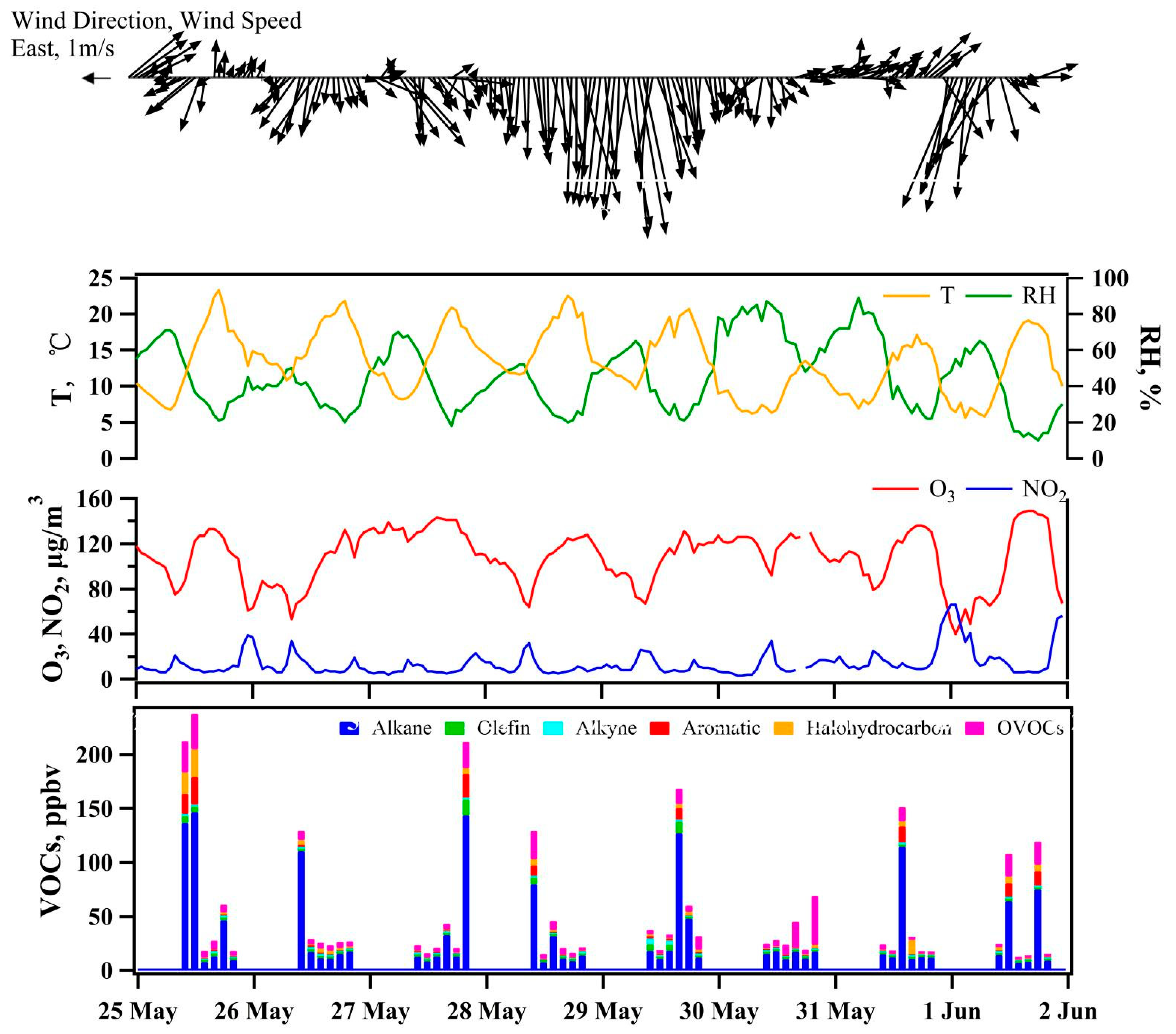
• Ozone changes in an apparent daily trend with a single peak, the VOC concentrations fluctuate significantly, and the pollution concentration and change characteristics of each component vary greatly. They were likely caused by multiple factors such as human activities on the ground and photochemical reactions. The urban areas of Lhasa were under transition conditions and controlled by both VOCs and NOx. Moreover, the most effective way to decrease ozone formation is to reduce the emissions of anthropogenic VOCs and NOx.
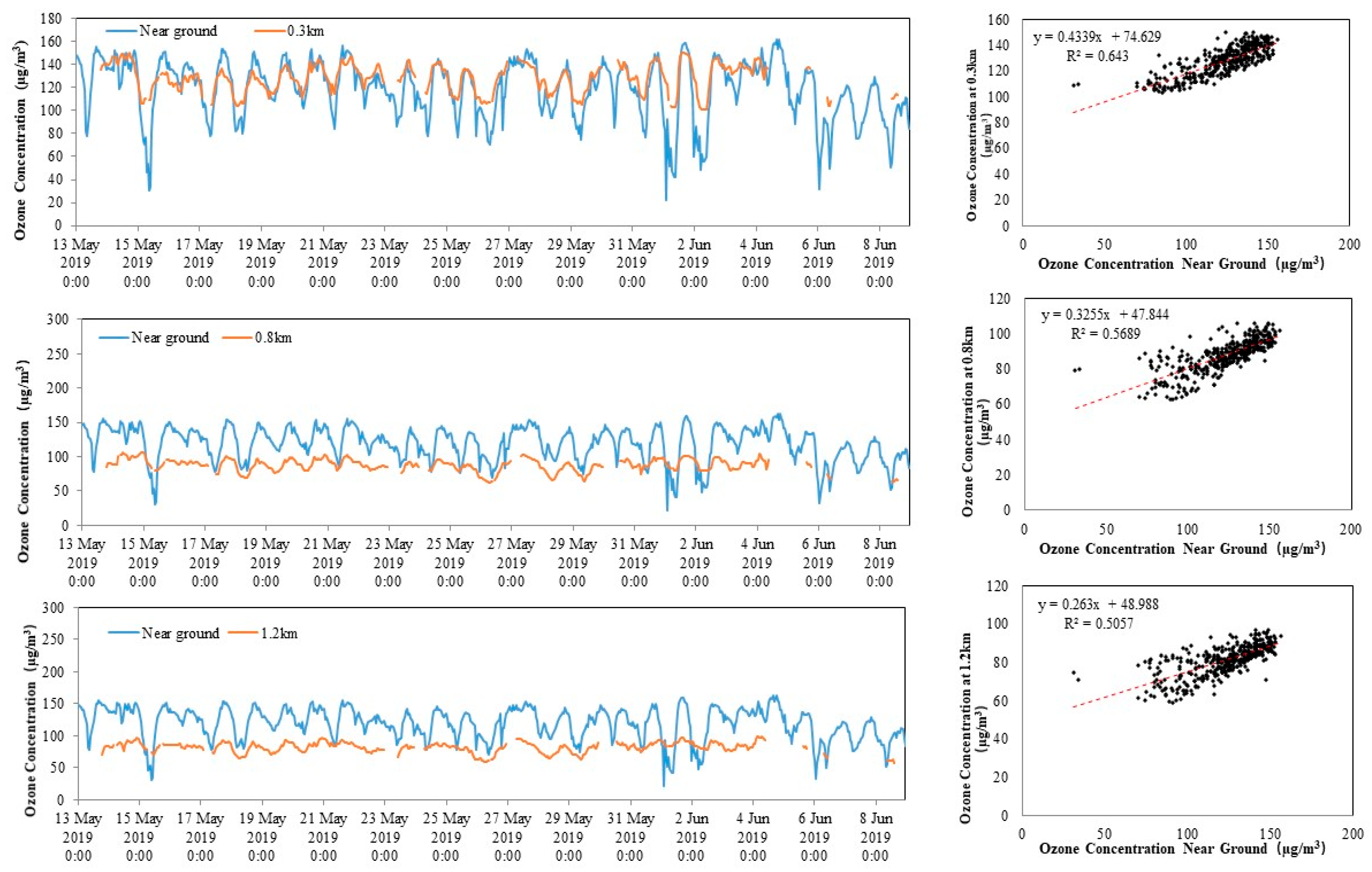
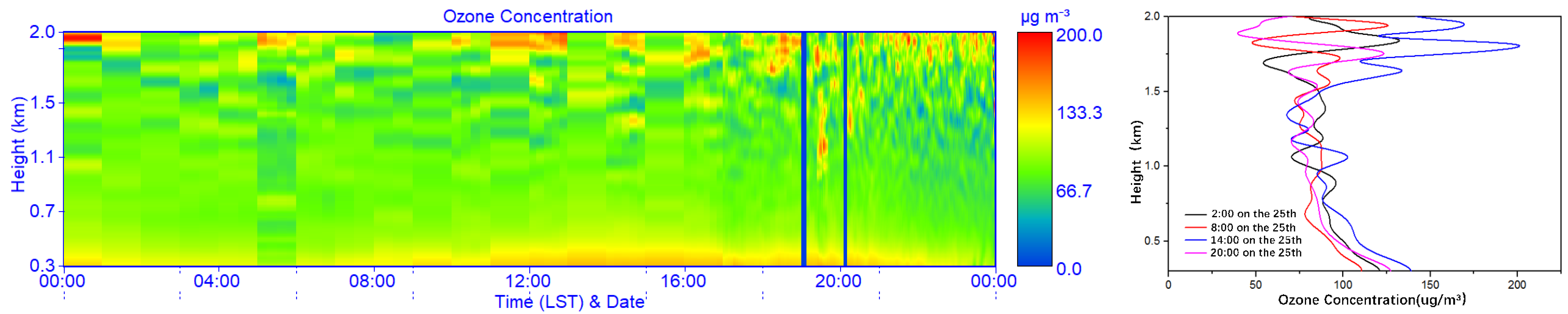
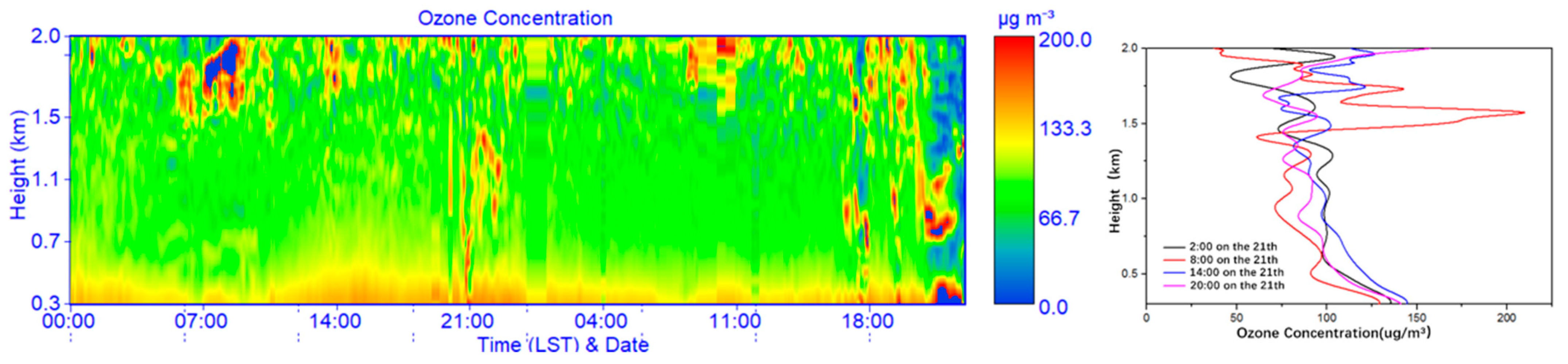
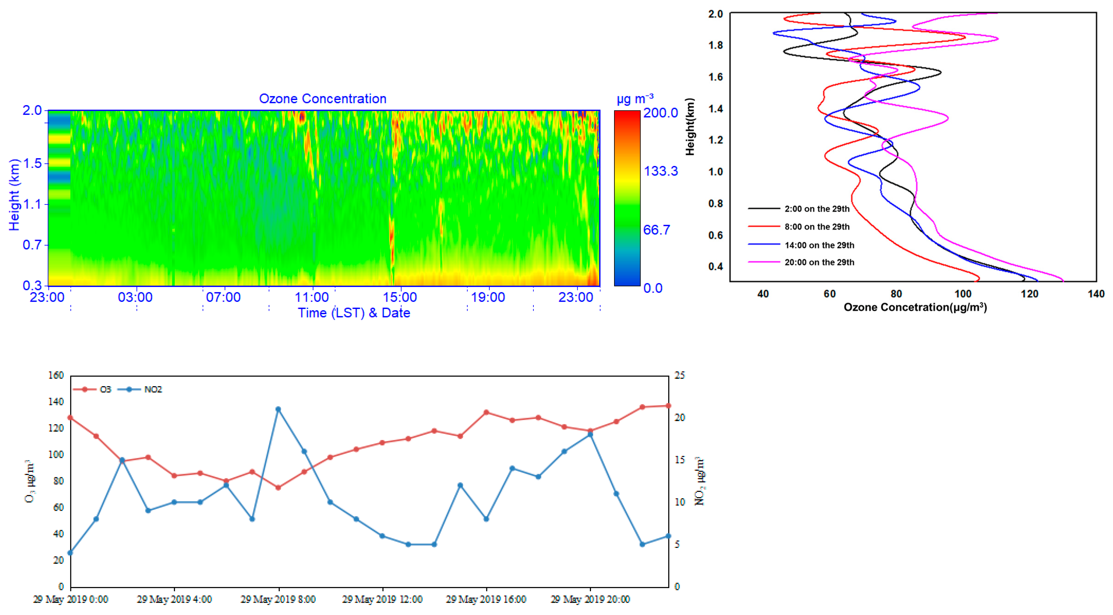
• From the perspective of the vertical distribution of near-ground ozone, the areas with high ozone concentrations in Lhasa are mainly concentrated within 400 m and carry apparent daily trends of an alternation. The changing ozone trends at different altitudes of 0.3 km, 0.5 km, and 1.2 km indicate that the vertical transmission of ozone is affected by the atmospheric boundary layer and the mixing difference caused by it. Because the photochemical reaction and a long time of sunshine are conducive to the generation and accumulation of ozone, high ozone concentrations occur from 12:00 to 23:00. Due to changes in diffusion and emission conditions, cumulative pollution exist both during the day and the previous night, and sometimes short-term titration also exists. The results also imply that Lhasa city is an essential source of ozone in the TP.
• The results are essential to understanding the formation and impacts of ozone in the TP.

References

1. Burkholder, J.B.; Cox, R.A.; Ravishankara, A.R. Atmospheric Degradation of Ozone Depleting Substances, Their Substitutes, and Related Species. Chem. Rev. 2015, 115, 3704–3759. [Google Scholar] [CrossRef] [PubMed]
2. Li, D.; Vogel, B.; Müller, R.; Bian, J.; Günther, G.; Li, Q.; Zhang, J.; Bai, Z.; Vömel, H.; Riese, M. High tropospheric ozone in Lhasa within the Asian summer monsoon anticyclone in 2013: Influence of convective transport and stratospheric intrusions. Atmos. Chem. Phys. 2018, 18, 17979–17994. [Google Scholar] [CrossRef] [Green Version]
3. Brook, R.D.; Franklin, B.; Cascio, W.; Hong, Y.; Howard, G.; Lipsett, M.; Luepker, R.; Mittleman, M.; Samet, J.; Smith, S.C.; et al. Air pollution and cardiovascular disease: A statement for healthcare professionals from the Expert Panel on Population and Prevention Science of the American Heart Association. Circulation 2004, 109, 2655–2671. [Google Scholar] [CrossRef] [PubMed]
4. Hallquist, M.; Wenger, J.C.; Baltensperger, U.; Rudich, Y.; Simpson, D.; Claeys, M.; Dommen, J.; Donahue, N.M.; George, C.; Goldstein, A.H.; et al. The formation, properties and impact of secondary organic aerosol: Current and emerging issues. Atmos. Chem. Phys. Discuss. 2009, 9, 3555–3762. [Google Scholar] [CrossRef] [Green Version]
5. Ma, Z.; Zhang, X.; Xu, J.; Zhao, X.; Meng, W. Characteristics of ozone vertical profile observed in the boundary layer around Beijing in autumn. J. Environ. Sci. 2011, 23, 1316–1324. [Google Scholar] [CrossRef]
6. Salmond, J.A.; McKendry, I.G. Secondary ozone maxima in a very stable nocturnal boundary layer: Observations from the Lower Fraser Valley, BC. Atmos. Environ. 2002, 36, 5771–5782. [Google Scholar] [CrossRef]
7. Shi, G.Y.; Bai, Y.B.; Iwasaka, Y.; Ohashi, T. A balloon measurement of the ozone vertical distribution over lahsa. Adv. Earth Sci. 2000, 15, 522–524. [Google Scholar]
8. Pazmiño, A.; Godin, S.; Wolfram, E.; Lavorato, M.; Porteneuve, J.; Quel, E.; Mégie, G. Intercomparison of ozone profiles measurements by a differential absorption lidar system and satellite instruments at Buenos Aires, Argentina. Opt. Laser Eng. 2003, 40, 55–65. [Google Scholar] [CrossRef]
9. Wang, L.; Follette-Cook, M.B.; Newchurch, M.J.; Pickering, K.E.; Pour-Biazar, A.; Kuang, S.; Koshak, W.; Peterson, H. Evaluation of lightning-induced tropospheric ozone enhancements observed by ozone lidar and simulated by WRF/Chem. Atmos. Environ. 2015, 115, 185–191. [Google Scholar] [CrossRef]
10. Chi, X.; Liu, C.; Xie, Z.; Fan, G.; Wang, Y.; He, P.; Fan, S.; Hong, Q.; Wang, Z.; Yu, X. Observations of ozone vertical profiles and corresponding precursors in the low troposphere in Beijing, China. Atmos. Res. 2018, 213, 224–235. [Google Scholar] [CrossRef]
11. Xing, C.; Liu, C.; Wang, S.; Chan, K.L.; Gao, Y.; Huang, X.; Su, W.; Zhang, C.; Dong, Y.; Fan, G. Observations of the vertical distributions of summertime atmospheric pollutants and the corresponding ozone production in Shanghai, China. Atmos. Chem. Phys. 2017, 17, 14275–14289. [Google Scholar] [CrossRef] [Green Version]
12. Zhu, B.; Hou, X.; Kang, H. Analysis of the seasonal ozone budget and the impact of the summer monsoon on the northeastern Qinghai-Tibetan Plateau. J. Geophys. Res. Atmos. 2016, 121, 2029–2042. [Google Scholar] [CrossRef] [Green Version]
13. Liang, W.; Yang, Z.; Luo, J.; Tian, H.; Bai, Z.; Li, D.; Li, Q.; Zhang, J.; Wang, H.; Ba, B. Impacts of the atmospheric apparent heat source over the Tibetan Plateau on summertime ozone vertical distributions over Lhasa. Atmos. Ocean. Sci. Lett. 2021, 14, 100047. [Google Scholar] [CrossRef]
14. Chen, Y.; Zhang, S.; Peng, C.; Shi, G.; Tian, M.; Huang, R.J.; Guo, D.; Wang, H.; Yao, X.; Yang, F. Impact of the COVID-19 pandemic and control measures on air quality and aerosol light absorption in Southwestern China. Sci. Total Environ. 2020, 749, 141419. [Google Scholar] [CrossRef]
15. Wang, X.; Zhang, T.; Xiang, Y.; Lv, L.; Fan, G.; Ou, J. Investigation of atmospheric ozone during summer and autumn in Guangdong Province with a lidar network. Sci. Total Environ. 2021, 751, 141740. [Google Scholar] [CrossRef]
16. Su, R.; Lu, K.; Yu, J.; Tan, Z.; Jiang, M.; Li, J.; Xie, S.; Wu, Y.; Zeng, L.; Zhai, C.; et al. Exploration of the formation mechanism and source attribution of ambient ozone in Chongqing with an observation-based model. Sci. China Earth Sci. 2018, 61, 23–32. [Google Scholar] [CrossRef]
17. Zhao, Z.-Y.; Cao, F.; Fan, M.-Y.; Zhang, W.-Q.; Zhai, X.-Y.; Wang, Q.; Zhang, Y.-L. Coal and biomass burning as major emissions of NOx in Northeast China: Implication from dual isotopes analysis of fine nitrate aerosols. Atmos. Environ. 2020, 242, 117762. [Google Scholar] [CrossRef]
18. Zhang, X.; Hu, B.; Wang, Y.; Zhang, W.; He, Y.; Sun, W. The analysis of variation characteristics and establishing of estimating equation for ultraviolet radiation in Lhasa. Chin. J. Atmos. Sci. 2012, 36, 744–754. [Google Scholar]
19. Wang, W.; van der A, R.; Ding, J.; van Weele, M.; Cheng, T. Spatial and temporal changes of the ozone sensitivity in China based on satellite and ground-based observations. Atmos. Chem. Phys. 2021, 21, 7253–7269. [Google Scholar] [CrossRef]
20. Xiong, C.; Wang, N.; Zhou, L.; Yang, F.; Qiu, Y.; Chen, J.; Han, L.; Li, J. Component characteristics and source apportionment of volatile organic compounds during summer and winter in downtown Chengdu, southwest China. Atmos. Environ. 2021, 258, 118485. [Google Scholar] [CrossRef]
21. Tan, Z.; Lu, K.; Jiang, M.; Su, R.; Dong, H.; Zeng, L.; Xie, S.; Tan, Q.; Zhang, Y. Exploring ozone pollution in Chengdu, southwestern China: A case study from radical chemistry to O3-VOC-NOx sensitivity. Sci. Total Environ. 2018, 636, 775–786. [Google Scholar] [CrossRef]
22. Xiu, T.; Sun, Y.; Sun, T.; Wang, Y. The vertical distribution of ozone and boundary layer structure analysis during summer haze in Beijing. Acta Sci. Circumstantiae 2013, 33, 321–331. [Google Scholar] [CrossRef]
23. Peng, L.; Gao, W.; Geng, F.; Ran, L.; Zhou, H. Analysis of Ozone Vertical Distribution in Shanghai Area. Acta Sci. Nat. Univ. Pekin. 2011, 47, 805–811. [Google Scholar] [CrossRef]
Figure 3. EKMA plot generated from the study period.
Remotesensing 14 02533 g003
Figure 6. Ozone concentration distribution and corresponding spatial line on lidar on 25 May. (Left) the changing trend of ozone concentration distribution and corresponding spatial line on lidar on 25 May; (Right) ozone concentration vs. height.
Remotesensing 14 02533 g006
Figure 7. Ozone 21–22 May represents typical cumulative ozone pollution. (Left) the changing trend of ozone concentration distribution; (Right) ozone concentration vs. height.
Remotesensing 14 02533 g007
Figure 8. Ozone vertical profile of ozone and the titration effect after local ozone formation. (Left) the changing trend of ozone concentration distribution and variations of ozone and NO2; (Right) ozone concentration vs. height.
Remotesensing 14 02533 g008