Article

A Satellite-Observed Substantial Decrease in Multiyear Ice Area Export through the Fram Strait over the Last Decade

1
Key Laboratory of Marine Geology and Environment, Institute of Oceanology, Chinese Academy of Sciences, Qingdao 266071, China
2
Center for Ocean Mega-Science, Chinese Academy of Sciences, Qingdao 266071, China
3
Laboratory for Marine Geology, Qingdao National Laboratory for Marine Science and Technology, Qingdao 266237, China
4
University of Chinese Academy of Sciences, Beijing 101408, China
*
Author to whom correspondence should be addressed.
Remote Sens. 2022, 14(11), 2562; https://doi.org/10.3390/rs14112562
Submission received: 6 April 2022 / Revised: 16 May 2022 / Accepted: 25 May 2022 / Published: 27 May 2022

Abstract

:
Revealing the changes in the Fram Strait (FS) multiyear ice (MYI) export is crucial due to their climate relevance in the context of the loss rate of MYI being faster than that of the total ice in the Arctic. Here, we estimated winter (October–April) MYI area export through the FS over the last 2 decades by using updated MYI concentration data retrieved from active and passive microwave satellite observations. We divided the period into two regimes relative to the ice index: D1 (2002/03–2010/11) and D2 (2012/13–2019/20). The observed variations of winter MYI exports D2 were compared with those of the previous decade D1. The results show that the MYI area exports display strong interannual variability. A significant decrease in MYI export for the periods between D1 and D2 is noted. On average, the wintertime MYI area exports declined sharply by 22% from 3.82 × 10⁵ km2 in D1 to 3.00 × 10⁵ km2 in D2. In addition, the percentage of MYI in the total sea ice outflow through the FS (PCM) also decreased distinctly from 72% in D1 to 59% in D2. Statistics show that weekly sea ice drift across the strait can explain 76% of the MYI area export variability. Furthermore, the dominant atmospheric drivers contributing to the decline in MYI area export during D2 were examined. In the last decade (D2), the strengthened low pressure in the North Atlantic sector, combined with an eastward shift in the axis of dipole anomaly (DA), resulted in reduced MYI advection from the Beaufort Sea and Siberian Coast toward the FS. Moreover, weakened cyclonic activity south of the FS also contributed to the reduction in MYI export during D2.

1. Introduction

Sea ice acts as a major component of the Arctic climate system through modulating the radiative flux, heat, and momentum exchanges between the ocean and atmosphere [1,2,3]. In the polar region, seasonal ice includes first-year ice (FYI, thickness greater than 30 cm) and young ice (YI, up to 30-cm thick). Multiyear ice (MYI) is ice that has survived one or more melt seasons. Arctic MYI is characterized by a greater thickness (typically above 2 m), higher albedo, smoother topographic features, and generally higher backscatter compared with seasonal ice since it is tolerant to surface melting [4]. The climatic significance of Arctic MYI can be attributed to its strong connection to summer ice coverage, as the remarkable decrease in winter MYI coverage is usually a precondition for a lower ice extent in the subsequent summers [5,6,7]. Therefore, the recent satellite-observed alarming retreat of MYI [7] requires the attention of a wide spectrum of communities in the context of shrinking Arctic sea ice cover in recent years.
The Arctic sea ice extent, obtained from the National Ice and Snow Data Center (NSIDC), decreased at a rate of −2.9 ± 0.4%/decade in February and −12.7 ± 2.0%/decade in September from 1979 to 2021. However, the decline in MYI cover is much larger. A prominent MYI area decline by −17%/decade was identified from 1979 to 2011 [8], whereas a more rapid decrease by −48%/decade was observed since the turn of the new century (2000–2017) [7]. Consequently, the sharp shrinkage of MYI cover gives rise to more coverage of seasonal ice in the Arctic Ocean. Specifically, MYI with an age of at least 2 years covered approximately 55% of the Arctic Basin in the 1980s [9] but shrank to approximately 30% in the recent decade [10]. The MYI coverage in the Arctic now retreats to a narrow band along the Canadian Arctic Archipelago (CAA) [7,10]. Since the current sea ice is younger and mechanically weaker, a higher sensitivity of sea ice variability to changes in atmospheric and oceanic forcing was identified [11,12,13,14].
Sea ice export is the crucial regulator of sea ice variability in the Arctic Ocean [15,16]. Sea ice, including MYI, can leave the Arctic Basin through a few defined gates, mainly including the Fram Strait (FS), Bering Strait, Gateway between Svalbard and Franz Josef Land (S-FJL), narrow channels of CAA, and Nares Strait. The FS serves as the primary outlet of the Arctic sea ice export, and the sea ice outflow through the other Arctic gateways is an order of magnitude smaller [15,16]. Previous estimates of the net annual sea ice volume (SIV) exported with the East Greenland Current via the FS amount to approximately 13% of the total sea ice mass in the Arctic Basin and approximately 90% of the total Arctic sea ice export [17].
In addition to the impacts on the Arctic sea ice mass budget, sea ice export through the FS, especially in cases with older and thicker MYIs, serves as a major source of surface freshwater for the Greenland–Iceland–Norwegian (GIN) seas, which is crucial for modulating the properties of dense water in the Nordic Seas. Variability in FS outflow can also modify the major water mass formation processes in the Greenland Sea, further downstream in the Subpolar North Atlantic, and is expected to have consequences on oceanic convective activity [18] associated with the Atlantic Meridional Overturning Current (AMOC) [19,20,21]. As global warming continues, understanding how MYI exports via FS have changed in recent decades is important to fully understand climate change in the Arctic.
Several studies have investigated the seasonal and interannual variability and long-term trend of sea ice export through the FS. Seasonally, over 80% of exported ice loss on average occurred during the cold season (October to May), while the sea ice outflow is typically lower in the warm season (June to September) due to the weakened sea-level pressure (SLP) gradients across the strait [22]. The long-term time series of FS sea ice area exports from 1935 to 2014 displays large interannual and multidecadal variability, although without a clear trend [23]. However, a distinct increasing SIC trend of 6%/decade was identifiable from 1979 to 2014 [23]. In addition, a discernible trend in SIV export via the FS was not observed during the period of 1979–2007 [24], and a significant negative trend (−648 ± 48 km3yr−1 per decade) was identified when the time series was extended to 1992–2014, which is largely attributed to thinning of the exported sea ice in the FS [25]. Although total sea ice export has been investigated in many studies, examinations of the variability and changes in MYI export through the FS are rare.
A large part of the sea ice export through the FS is related to the Beaufort Gyre and the Transpolar Drift Stream (TDS). The two systems are associated with large-scale atmospheric circulations, such as the Arctic Oscillation (AO) and Dipole Anomaly (DA) [16,26]. When the Beaufort Gyre is strong, anticyclonic ice circulation is enhanced, and sea ice, including MYI, tends to stay inside the Arctic Basin. As a consequence, the FS sea ice export is reduced. In contrast, during the weak Beaufort Gyre, sea ice associated with the TDS is advected from the Siberian coast toward the FS. In this situation, the FS features a comparably higher sea ice export [23]. Additionally, wind variability associated with the DA may influence MYI export via the FS through its modulation of TDS [16]. The role of these large-scale atmospheric forcings on MYI export changes over the last 2 decades begs for further investigation. In addition, the contribution of synoptic forcing (cyclone) to MYI export variability remains unclear.
In this paper, we use an updated record of MYI concentrations derived from active and passive satellite observations [27,28] to evaluate winter (October to April) MYI exports through the FS over approximately the past 2 decades. We also divided the 2 decades into two regimes based on an index that the percentage coefficient of MYI in the total sea ice exported via the FS (PCM). The observed variations of MYI exports in the last decade (D2 with high PCM, 2012/13–2019/20) were compared with those in the earlier decade (D1 with low PCM, 2002/03–2010/11). Furthermore, we elucidate their linkages with ice drift patterns, MYI coverage in the Arctic Basin, and varying atmospheric circulation patterns. The results of this study will deepen the understanding of the variability and changes regarding MYI exports through the FS and its driving atmospheric factors. This study is organized as follows. The datasets used in this paper and the methodology applied to retrieve MYI concentrations are described in Section 2. Among them, techniques to quantify MYI exports are introduced. Section 3 depicts the records and variability in MYI area exports through the FS. Section 4 discusses the linkages between MYI area exports and driving atmospheric factors. Finally, the conclusion is presented in Section 5.

2. Data and Methodology

2.1. Data

The MYI concentration was retrieved from passive and active microwave remote sensing observations and in a two-step procedure using the Environment Canada Ice Concentration Extractor (ECICE) system [29,30] and several correction schemes [27,28]. The ECICE algorithm with input brightness temperature in several frequency channels at both horizontal (H) and vertical (V) polarization are obtained from the sensor AMSR-E (Advanced Microwave Scanning Radiometer for EOS) on the NASA satellite Aqua (until May 2011), or AMSR2 (Advanced Microwave Scanning Radiometer 2) on the JAXA satellite GCOM-W1 (since September 2011) and backscatter coefficients are obtained from the QuikSCAT (2002 to early 2009) or from ASCAT (late 2009 to present).
The ECICE algorithm starts with a linear mixing model [29,30] that decomposes each input observation into contributions from each surface type (in this case MYI, FYI, YI, and open water (OW)) weighted by the concentration of the surface type within the sensor’s field of view. Four input observations are used in the ECICE algorithm: normalized radar backscattering cross section at C band from ASCAT, brightness temperatures at 36.5 GHz vertical and horizontal polarization channels (TB,37V and TB,37H) from AMSR-E or AMSR2, and gradient ratio of 36.5 GHz and 18.7 GHz vertical polarization channels (GR37V,19V). GR37V,19V is defined as:
G R 37 V , 19 V = T B , 37 V T B , 19 V T B , 37 V + T B , 19 V      
Based on the known distributions of ice types, interpreted as probability density functions, a number n of possible realizations of typical brightness temperatures and normalized radar backscattering cross section for the four surface types is randomly generated. Then, the median of the n solutions for the area fractions is the final result. Note that ECICE algorithm works only during the freezing season since the surface properties of all ice types change drastically and become similar in the melt season. More details can be found in Shokr, Lambe [30]. The MYI correction schemes also use surface temperature data from the ERA-Interim reanalysis [31] and sea ice motion (SIM) from the NSIDC [32] or the Satellite Application Facility on Ocean and Sea Ice (OSISAF) [33] to correct misclassifications by ECICE caused by melt, refreezing, snow metamorphosis, and sea ice drift.
The MYI concentration data was tested and verified by comparison with a high-resolution synthetic aperture radar (SAR). Compared with Radarsat-1 SAR images in the Greenland Sea and FS, this MYI dataset is accurate and reliable [28]. Moreover, young ice streaks with high backscatter and streaks of low values often appear in the southwest of Svalbard, which was probably generated locally due to wind and low temperature. Both active and passive microwave observations mistakenly identified this young ice as MYI. These MYI correction schemes can still correct this classification [28]. Admittedly, some problems remain: weather influence on the surface of the MYI may cause considerable day-to-day fluctuation in MYI concentration, which could be substantially reduced in the monthly mean data. In the Kara Sea and the Laptev Sea, unrealistically high MYI concentrations occur from March to May, which are probably caused by small areas of rough YI with wet snow. However, it has little impact on our results because MYI area exports through the FS are determined by the MYI across the gate The MYI observations were obtained from the University of Bremen and cover October 2002 to the present except for the wintertime of 2011/2012 because of the gap in the operational periods between AMSR-E and AMSR2.
The daily satellite-derived sea ice concentration (SIC) and SIM are used to obtain the sea ice area flux via the FS. The SIC field, gridded on an equal-area polar stereographic projection (25 km × 25 km), is the latest version of the product (v3.1) [34]. Multiple passive microwave observations, including SMMR, SSM/I, and SSMIS, are used to derive the SIC fields by applying the bootstrap algorithm to the passive microwave brightness temperatures. Daily SIM vectors projected onto the 25-km Northern Hemisphere Equal-Area Scalable Earth Grid are derived from a variety of input sources, including observations from spaceborne sensors (AVHRR, AMSR-E, SMMR, SSMI, and SSMI/S), measurements from International Arctic Buoy Programme (IABP) buoys, and estimates from the reanalysis winds provided by the National Centers for Environmental Prediction (NCEP)/National Center for Atmospheric Research (NCAR) [35]. The SIC and SIM datasets are both obtained from the NSIDC.
Large-scale atmospheric oscillations such as the AO, North Atlantic Oscillation (NAO), and Arctic DA are used to investigate the possible linkages with the variability in MYI area exports through the FS. The AO and NAO indices are provided by the Climate Prediction Center (CPC) at the National Oceanic and Atmospheric Administration (NOAA). The SLP is obtained from the latest European Center for Medium Range Weather Forecasts (ECMWF) reanalysis version 5 (ERA5) with a 1° × 1° grid [36], and it is used to analyze atmospheric circulation. All the data used here span a period from 2002 to 2020.

2.2. Methodology

2.2.1. Sea Ice Area Flux Estimates

Here, the MYI area export flux in winter (October to April) through the FS (Figure 1) is estimated as the integral of the product of gate-perpendicular SIM and MYI concentrations for all grid points across the corresponding gate. The daily estimate of sea ice area flux (F, km2/day) is calculated as
F = i = 1 N u i c i Δ x T ( i = 1 , 2 , , N )      
where u corresponds to the gate-perpendicular SIM (km/s), c denotes MYI concentration, Δx represents the width of a grid (25 km), T is seconds in a day, and i (1, 2… N) refers to the index of grid cells along the gate. The monthly area flux (Fm) is the sum of daily fluxes for the corresponding calendar month. In addition, a two-tailed Student′s t-test was also performed to test the confidence level of the correlation coefficient between MYI area export time series and its related factors. Statistical significance is reported at or over the 95% confidence level.
Winter ice export plays a dominant role in the MYI mass balance in the Arctic because the sea ice outflow is typically low during the summer months when SLP gradients across the strait are weaker [15]. In addition, summer MYI concentrations from observations are not available due to the masked difference between FYI and MYI backscatters associated with surface melt. Therefore, we only focus on ice export through the FS in winter when the retrieved MYI concentration is physically credible. Consequently, since we consider the winter flux of MYI only, the obtained values are less than the annual MYI exports.

2.2.2. Uncertainty of Sea Ice Area Flux

The uncertainty of the daily area flux can be expressed as follows [37]:
σ F = σ d L N    
where L represents the width of the considered outlet and σd is the uncertainty in the displacement estimates over the time step and is obtained as 1.73 km/day [38], which is estimated by comparing SIM data from the NSIDC with buoy drifts. N is the number of independent samples across the gate. The uncertainty in the seasonal (σ) area flux estimates can be described as
σ = σ F N D      
where ND denotes the days for the period examined. Based on these equations, the expected uncertainties for the area export are obtained.

2.2.3. MYI Export Index

For each month’s (season’s) MYI average area in the Arctic Ocean, the daily area for each day of the month is first calculated from the daily gridded input data using a threshold MYI concentration value (15% or 50%) cutoff and size of each grid cell. Then, the monthly (seasonal) area value is obtained by simply averaging the daily (monthly) area over the corresponding month (season). Note that the MYI concentration within a small extent covering the Arctic Pole Hole is absent due to the satellite observational inclination, and the grids in the Pole Hole are discarded in calculating Arctic MYI Area. A normalized MYI export index (MI) is introduced to examine the variability and extremes in monthly MYI area export through the FS. The time series of MI is constructed by
MI ( t ) = F ( t ) F ¯ σ F  
where F ( t ) is the monthly MYI area export through the Fram Strait and F ¯ and σ F are the mean and standard deviation of the monthly MYI area flux over the target period, respectively.

2.2.4. Cyclone Activity Index

A cyclone represents an intense synoptic activity, is a common atmospheric forcing in the Arctic throughout the year [39], and can largely determine the variability of sea ice export through the Fram Strait [40]. In addition, winter cyclones occur frequently in the south of the Fram Strait, near the Icelandic low-pressure area [41]. Thus, the impacts of cyclone activity on MYI area export changes between the two regimes are investigated. The cyclone characteristics are generally described with the cyclone intensity, cyclone trajectory count, and cyclone duration, which describe a particular aspect of cyclone activity. Here we use an integrative index, the cyclone activity index (CAI), which represents a combination of those parameters [42]. The CAI is defined as the sum over all cyclone centers at a 6-hourly resolution for the differences between the central SLP of the cyclone and the climatological seasonal mean SLP at corresponding grid points in a particular region during winter.

3. Results

3.1. MYI Area Export through the FS

The variability in MYI and total sea ice area export through the FS in winter (October–April) over the last nearly 2 decades of the record is shown in Figure 2. The mean and trend in ice export flux corresponding to Figure 2 were obtained and are summarized in Table 1. The observed variations of MYI export flux in the latter decade D2 with low PCM were compared with those in the earlier decade D1 with high PCM.
Table 1 shows that both MYI and total sea ice exports had a significant increasing trend during D1 (0.14 × 10⁵ km2/yr for MYI and 0.28 × 10⁵ km2/yr for total sea ice) and no significant trend during D2. Together, there is no significant trend over the last two decades for either MYI export or total sea ice outflow. Regarding decadal changes, the mean winter MYI export declined substantially, by approximately 22%, from 3.82 ± 0.48 × 10⁵ km2 in D1 to 3.00 ± 0.75 × 10⁵ km2 in D2. Using Equations (3) and (4), the expected mean uncertainty in the cumulative sea ice export during winter is estimated to be 5.4 × 10³ km2. This value amounts to 1.6% of the average MYI area flux over the whole period.
MYI exports decreased even more than seasonal ice exports. The mean PCM decreased from 72% in D1 to 59% in D2. The discrepancy between the exported change in MYI and seasonal ice indicates that the MYI export has its own variability, which differs from the total ice export. The driving processes causing the MYI export changes, including the MYI area remaining in the Arctic Basin, MYI drift pattern, and atmospheric circulation, may not be consistent with those leading to fluctuations in total ice export. Here, we attempt to focus on the linkages between MYI area export variability and these factors. Finally, the primary causes related to the significant decline in decadal MYI exports via the FS will be discussed.

3.2. Seasonal Cycle of MYI Area Export

The mean seasonal cycle of MYI area export through the FS (Figure 3) is characterized by a maximum of 6.64 ± 2.19 × 10⁴ km2 (5.69 ± 2.87 × 10⁴ km2) in March and a minimum of 4.27 ± 1.26 × 10⁴ km2 (3.27 ± 1.14 × 10⁴ km2) in April in D1 (D2) (see also Table 2). The mean annual cycle shows lower flux in D2 relative to that in D1, with a maximum reduction during January (Figure 3c). In addition, monthly MYI area exports strongly vary between 5.75 ± 2.77 × 10⁴ km2 in October and 4.27 ± 1.26 × 10⁴ km2 in April during D1 and vary between 5.80 ± 2.92 × 10⁴ km2 in December and 3.27 ± 1.14 × 10⁴ km2 in April during D2. The monthly standard deviation in D2 increased significantly in December and decreased obviously in October compared with that in D1.
The mean seasonal cycle of the total sea ice area export over the entire period is related to that of MYI (R = 0.74). The PCM is characterized by a maximum in October (87% in D1 and 67% in D2) and a minimum in April (57% in D1 and 48% in D2). The PCM also evidently shows a decline in D2 compared with that in D1, especially from October to December, with an average of −20%. These results reaffirm that the decrease in MYI export through the FS, compared with the changes in total sea ice outflow, is characterized by its own anomaly and is possibly associated with different atmospheric forcing behaviors.

3.3. Variability in Monthly MYI Area Export

To place the MYI area export into a broader context, the monthly MYI concentration and drift patterns in the Arctic Ocean are examined. Here we only chose the four most positive/negative events in D1 and D2, respectively (Figure 4). The results showed that the positive anomalies of MYI area exports featured different large-scale MYI anomaly fields and ice circulation patterns (Figure 4a). In other words, intraseasonal variations in MYI area exports through the FS seem to be insensitive to varying sea ice drift patterns. This inconsistency of the sea ice drift pattern among these large or low export cases is further illustrated in D2 (Figure 4b). Because the MYI area export via the FS is essentially calculated by the local MYI drift and concentration. It indicates that the seasonal ice drift pattern upstream in the Fram Strait is insensitive to large-scale ice circulation in the Arctic Ocean. This finding is consistent with the previous arguments that local variations such as the SLP difference across the strait and/or the intensity and position of the TDS [24] explain a larger fraction of the variance in sea ice export.

3.4. Influence of MYI Distribution and Motion on MYI Export

As the source of MYI export, the MYI area in the Arctic Ocean is calculated in this section. The mean Arctic MYI areas in the winter season with 15% and 50% as cutoffs for the lowest MYI concentration are shown in Figure 5a. The variability between the two areas is consistent except for the difference in magnitude, indicating that the MYI area calculated with a 15% threshold did not noticeably increase the uncertainty due to the threshold being small. We choose 15% as the threshold of MYI concentration to estimate the Arctic MYI area in the following analysis. The result shows a significant retreat trend (−1.55 × 10⁵ km2/yr) in Arctic MYI area during D1, while the MYI area export has a positive trend during the same period (Figure 2 and Figure 5a). Thus, an increased MYI export seems to partly contribute to the significant retreat trend of Arctic MYI cover in D1, which needs to be further investigated. The Arctic MYI area has no trend during D2. In addition, the percentage of MYI area exported through the FS to the Arctic MYI area decreased from D2 (10%) to D2 (8%), which helped slow the loss of the Arctic MYI.
Possible causality relationships between the area of MYI cover in the Arctic ocean and MYI export via FS were also examined on an intraseasonal scale. Monthly Arctic MYI area and MYI area export from 2002 to 2020 are used in the lagged correlation. The result shows that the MYI area export lags Arctic MYI area anomalies by 5 to 6 years (Figure 5b), which suggests that changes in Arctic MYI cover significantly contribute to the MYI area export via FS with the greatest impact after half a decade.
To evaluate the impacts of ice drift and MYI concentration across-gate on MYI area export, we calculate the simple linear regression between MYI area export and ice drift and MYI concentration using weekly observations. The result shows that the correlation coefficient between MYI concentration and MYI area export is 0.53, which explains 28% of the variability in MYI area export, and the correlation coefficient between ice drift and MYI area export is 0.87, which can explain 76% of the variance in MYI area export (Figure 6). The stronger correlation indicates that local ice drift in the FS has a more significant effect on MYI export than the MYI concentration. Previous research shows that the total sea ice export is also primarily determined by sea ice drift, which can explain more than 90% [43]. Therefore, MYI export through the FS is largely related to atmospheric circulation since ice drift is largely wind-driven [24]. This aspect is further analyzed in the following text.

4. Discussion

To further examine the drivers of the variability in MYI export via the FS in a broad context, the averaged wintertime fields in terms of MYI concentration, SLP, and ice drift during D1 and D2 are constructed (Figure 7). The results show that the MYI coverage is mainly located along the band of northern CAA and Greenland, with most MYI concentrations being less than 20% over the marginal seas (Figure 7a,b). The positions of the mean high- (in the central Beaufort Sea) and low- (in North Atlantic) pressure centers allow the winds to drive the sea ice flow. In particular, the SLP pattern in D2 (Figure 7b) reveals a negative pressure anomaly over the Atlantic sector that expanded toward the Beaufort Sea. Considering the large-scale atmospheric circulation, this pattern results in cyclonic circulation primarily around the Arctic Basin, with a similar response in sea ice transport. The pronounced decadal changes between D1 and D2 include strengthening of the Beaufort Gyre, accumulation of MYI over the East Siberian Sea, and enhanced ice import from the Laptev Sea into the Arctic Basin (Figure 7c). That the Beaufort Gyre strengthened in the last decade is in accordance with previous studies [44,45]. Consequently, more MYI was found north of the CAA, extending to the central Arctic, as well as a negative MYI anomaly along the area of the TDS due to the lower availability of MYI sources.
The TDS provides the main source of sea ice outflow through the FS. Therefore, the shrinkage of MYI coverage over the TDS regime (Figure 7c) led to a decrease in the MYI coverage exported through the FS and was associated with a decrease in MYI area export, as observed in D2 (Table 1 and Figure 2). Moreover, the sea ice drift through the FS showed the opposite tendency between D1 and D2 (Figure 7c): an intensified outflow on the west side (near Greenland) and weakened outflow on the east side (near Svalbard). Together, the negative export anomaly dominates the positive anomaly (−12.7 km/d vs. 8.3 km/d). Thus, the east–west contrasting ice drift tendency was favorable for the decreased MYI export during D2.
Three typical large-scale atmospheric circulation modes are investigated for possible linkages with the variability in MYI area export. AO corresponds to the leading mode of the empirical orthogonal function (EOF) of SLP north of 20°N [46]. The NAO is referred to as the SLP leading mode over the North Atlantic [47]. DA corresponds to the second-leading mode of SLP north of 70°N [26]. AO and NAO represent the dominant factors associated with Arctic sea ice movement and increased FS export, which was particularly prominent in the mid−1990s [48,49]. Wind variability associated with DA can influence sea ice export through the FS via the impact on the TDS [26,43,50].
The correlations between monthly MYI area export and AO and NAO are all less than 0.2 (119 samples) from lag 0 to 7 months (Figure 8a), which is consistent with Smedsrud, Halvorsen [23]. They found that the relationship between the AO index and winter FS ice export does not appear to be stationary over time because the AO spatial pattern does not exhibit strong pressure gradients in the FS. Therefore, the AO includes characteristics of the NAO, which is regionally bounded [51]. In contrast, the correlation coefficient between the MYI area export and DA was 0.40 by lag 0 month with a 95% confidence level; it was 0.49 during D1 and 0.27 during D2 (not shown). The decrease in the correlation between DA and MYI area export in the last decade may be related to change in spatial structure of the DA. The axis of DA along the dateline, as seen in Figure 8b, shifted toward the east in D2, which tends to reduce advection of ice from the Beaufort Sea and Siberian Coast toward the FS and contribute to the decline in MYI area export.
In addition to the above factors, the effect of cyclones on MYI export is also examined. Cyclones play a vital role with both dynamic and thermodynamic impacts on ice export through the FS, especially considering the drastic retreat and thinning of Arctic sea ice cover since the 2000s. As the most significant external force to SIM, the intensified surface wind stress during a cyclone process could modify the local ice drift and accordingly affect the FS MYI export [40]. Furthermore, the cyclone intensity is greater during the cold season than during the warm season throughout the Arctic region [42]. To examine the role of cyclone activity in the decrease in MYI area export, an integrated CAI was used. The CAI synthesizes information including the frequency, intensity, and duration of a cyclone into a comprehensive index to depict the impacts of cyclone activity [42].
Clearly, cyclones occur more frequently in the area from southwest Iceland through the Norwegian Sea toward the Kara Sea (Figure 9a,b), which is also one of the three typical pathways by which Northern Hemisphere extratropical cyclones propagate northward into the Arctic during winter [42]. The cyclonic activity associated with intensified surface wind stress in this pathway plays a vital role in driving sea ice drift from the Arctic Ocean through FS into the GIN Sea. Figure 9c shows the temporal changes between D1 and D2 and indicates that the cyclone tracks generally shifted to the southeast with weaker CAI south of the FS and enhanced CAI in the Kara Sea. The shifted cyclonic activity would reduce ice outflow through the FS and could be responsible for the decrease in winter MYI export in D2.

5. Conclusions

In this study, we estimated the wintertime MYI area exports through the FS for approximately the last 2 decades by using the updated MYI concentration data retrieved from passive (AMSR-E and AMSR2) and active (QuikSCAT and ASCAT) microwave satellite observations. The variability and decadal changes in the winter MYI export flux in the latter decade (D2, 2012/13–2019/20) were compared with those in the earlier decade (D1, 2002/03–2010/11). Moreover, the factors contributing to the variability in MYI area exports are investigated.
Overall, there is no trend in MYI area exports through the FS over the last nearly 2 decades. A significant increasing trend of MYI export was encountered during D1 (0.14 × 10⁵ km2/yr). A dramatic decline of 22% is observed for the mean MYI exports from 3.82 ± 0.48 × 10⁵ km2 during D2 to 3.00 ± 0.75 × 10⁵ km2 during D1. Notably, the MYI exports through the strait decreased even more than the total ice exports between the two decades. The PCM decreased distinctly from 72% during D1 to 59% during D2.
The driving processes, including MYI coverage in the Arctic Basin, across-strait ice drift and MYI concentration, large-scale atmospheric circulation, and cyclone activity, were investigated to examine the variability in MYI area export and decadal changes in MYI export between D2 and D1. Compared with the local MYI concentration, local ice drift in the FS has a more significant effect on MYI export that its variability can explain 76% of the variance in MYI area export. The changes in Arctic MYI cover also contribute to the MYI area export variability, with a lag of 5 years. Relative to D1, the negative pressure anomaly in the Atlantic sector expanded toward the Beaufort Sea during D2, resulting in large-scale changes in the intensity and character of ice transport in the Arctic Basin. The pronounced changes include a strengthening of the Beaufort Gyre, MYI accumulation in the East Siberian Sea, and enhanced ice import from the Laptev Sea into the Arctic Basin. Consequently, more MYI appears north of the CAA extending to the central Arctic, and a negative MYI anomaly occurs along the area of the TDS. These findings favor the decrease in MYI area exports in the last decade.
In addition, the connection of MYI export with AO(NAO) is weak. In contrast, MYI exports are significantly correlated with DA, although the role of DA in driving exports was weakened in D2. Moreover, the DA axis shifted eastward in D2, resulting in reduced ice advection from the Beaufort Sea and Siberian Coast toward the FS and contributing to the decline in MYI area export. Considering the synoptic atmospheric forcing, the weakened cyclonic activity with a lower CAI south of the FS could also be responsible for the decrease in winter MYI export. Since the large retreat of the MYI area in the Arctic is alarming to climate change communities, knowledge of the dramatic changes due to export variability is compelling. The results of this study provide a comprehensive picture of the variability in MYI area export and its driving processes, which are critical to understanding the relationship between rapid climatic change and large sea ice loss in the Arctic Ocean.

Author Contributions

Y.W. and H.B. conceived of the idea for the protocol and experimental design. H.B. provided primary support and guidance on the research. Y.W. and Y.L. performed data processing. All authors have read and agreed to the published version of the manuscript.

Funding

This work is supported by the National Natural Science Foundation of China (42106223; 42076185), the Natural Science Foundation of Shandong Province, China (ZR2021QD059; ZR2020MD100), the China Postdoctoral Science Foundation (2020TQ0322), the key projects of Pilot National Laboratory for Marine Science and Technology (Qingdao) (2022QNLM010204), the Open Funds for the Key Laboratory of Marine Geology and Environment, Institute of Oceanology, Chinese Academy of Sciences (MGE2021KG15; MGE2020KG04), and the Key Deployment Project of Centre for Ocean Mega-Research of Science, Chinese Academy of Sciences (COMS2020Q12).

Data Availability Statement

We thank the University of Bremen for providing MYI concentration data (https://seaice.uni-bremen.de/multiyear-ice/, accessed on 20 August 2021). The SIC and SIM datasets are both obtained from the NSIDC (https://nsidc.org/data/NSIDC-0079). The SLP from ERA5 can be obtained from the ECMWF (https://cds.climate.copernicus.eu/cdsapp#!/search?type=dataset, accessed on 20 August 2021). The AO and NAO indices are provided by the Climate Prediction Center (CPC) at the National Oceanic and Atmospheric Administration (NOAA) (https://www.cpc.ncep.noaa.gov/products/precip/CWlink/daily_ao_index/teleconnections.shtml, accessed on 20 August 2021).

Conflicts of Interest

The authors declare no conflict of interest.

References

  1. Porter, D.F.; Cassano, J.J.; Serreze, M.C. Analysis of the Arctic atmospheric energy budget in WRF: A comparison with reanalyses and satellite observations. J. Geophys. Res. Atmos. 2011, 116, D22108. [Google Scholar] [CrossRef]
  2. Smith, D.M.; Dunstone, N.J.; Scaife, A.A.; Fiedler, E.K.; Copsey, D.; Hardiman, S.C. Atmospheric response to Arctic and Antarctic sea ice: The importance of ocean–atmosphere coupling and the background state. J. Clim. 2017, 30, 4547–4565. [Google Scholar] [CrossRef]
  3. Peterson, A.K.; Fer, I.; McPhee, M.G.; Randelhoff, A. Turbulent heat and momentum fluxes in the upper ocean under Arctic sea ice. J. Geophys. Res. Ocean. 2017, 122, 1439–1456. [Google Scholar] [CrossRef]
  4. Perovich, D.K.; Polashenski, C. Albedo evolution of seasonal Arctic sea ice. Geophys. Res. Lett. 2012, 39, 8501. [Google Scholar] [CrossRef]
  5. Overland, J.E.; Wang, M. When will the summer Arctic be nearly sea ice free? Geophys. Res. Lett. 2013, 40, 2097–2101. [Google Scholar] [CrossRef]
  6. Polyakov, I.V.; Walsh, J.E.; Kwok, R. Recent changes of Arctic multiyear sea ice coverage and the likely causes. Bull. Am. Meteorol. Soc. 2012, 93, 145–151. [Google Scholar] [CrossRef]
  7. Kwok, R. Arctic sea ice thickness, volume, and multiyear ice coverage: Losses and coupled variability (1958–2018). Environ. Res. Lett. 2018, 13, 105005. [Google Scholar] [CrossRef]
  8. Comiso, J.C. Large Decadal Decline of the Arctic Multiyear Ice Cover. J. Clim. 2012, 25, 1176–1193. [Google Scholar] [CrossRef]
  9. Tschudi, M.; Meier, W.N.; Stewart, J.S.; Fowler, C.; Maslanik, J. EASE-Grid Sea Ice Age; Version 4; [Indicate subset used]; NASA National Snow and Ice Data Center Distributed Active Archive Center: Boulder, CO, USA, 2019. Available online: https://nsidc.org/data/nsidc-0611/versions/4 (accessed on 20 August 2021).
  10. Bi, H.; Yu, L.; Yunhe, W.; Xi, L. Arctic multiyear sea ice variability observed from satellites: A review. J. Oceanol. Limnol. 2020, 38, 962–984. [Google Scholar] [CrossRef]
  11. Thackeray, C.W.; Hall, A. An emergent constraint on future Arctic sea-ice albedo feedback. Nat. Clim. Chang. 2019, 9, 972–978. [Google Scholar] [CrossRef]
  12. Kashiwase, H.; Ohshima, K.I.; Nihashi, S.; Eicken, H. Evidence for ice-ocean albedo feedback in the Arctic Ocean shifting to a seasonal ice zone. Sci. Rep. 2017, 7, 8170. [Google Scholar] [CrossRef] [PubMed]
  13. Olonscheck, D.; Mauritsen, T.; Notz, D. Arctic sea-ice variability is primarily driven by atmospheric temperature fluctuations. Nat. Geosci. 2019, 12, 430–434. [Google Scholar] [CrossRef]
  14. Niederdrenk, A.L.; Notz, D. Arctic sea ice in a 1.5 C warmer world. Geophys. Res. Lett. 2018, 45, 1963–1971. [Google Scholar] [CrossRef] [Green Version]
  15. Krumpen, T.; Gerdes, R.; Haas, C.; Hendricks, S.; Herber, A.; Selyuzhenok, L.; Smedsrud, L.; Spreen, G. Recent summer sea ice thickness surveys in Fram Strait and associated ice volume fluxes. Cryosphere 2016, 10, 523–534. [Google Scholar] [CrossRef] [Green Version]
  16. Wang, Q.; Ricker, R.; Mu, L. Arctic sea ice decline preconditions events of anomalously low sea ice volume export through Fram Strait in the early 21st century. J. Geophys. Res. Ocean. 2021, 126, e2020JC016607. [Google Scholar] [CrossRef]
  17. Haine, T.W.N.; Curry, B.; Gerdes, R.; Hansen, E.; Karcher, M.; Lee, C.; Rudels, B.; Spreen, G.; de Steur, L.; Stewart, K.D.; et al. Arctic freshwater export: Status, mechanisms, and prospects. Glob. Planet Chang. 2015, 125, 13–35. [Google Scholar] [CrossRef] [Green Version]
  18. Karcher, M.; Gerdes, R.; Kauker, F.; Koberle, C.; Yashayaev, I. Arctic Ocean change heralds North Atlantic freshening. Geophys. Res. Lett. 2005, 32, 5. [Google Scholar] [CrossRef] [Green Version]
  19. Chen, X.; Tung, K.-K. Global surface warming enhanced by weak Atlantic overturning circulation. Nature 2018, 559, 387–391. [Google Scholar] [CrossRef]
  20. Yang, Q.; Dixon, T.H.; Myers, P.G.; Bonin, J.; Chambers, D.; Van den Broeke, M.R.; Ribergaard, M.H.; Mortensen, J. Recent increases in Arctic freshwater flux affects Labrador Sea convection and Atlantic overturning circulation. Nat. Commun. 2016, 7, 10525. [Google Scholar] [CrossRef] [Green Version]
  21. Mahajan, S.; Zhang, R.; Delworth, T.L. Impact of the Atlantic Meridional Overturning Circulation (AMOC) on Arctic Surface Air Temperature and Sea Ice Variability. J. Clim. 2011, 24, 6573–6581. [Google Scholar] [CrossRef] [Green Version]
  22. Tsukernik, M.; Deser, C.; Alexander, M.; Tomas, R. Atmospheric forcing of Fram Strait sea ice export: A closer look. ClDy 2010, 35, 1349–1360. [Google Scholar] [CrossRef] [Green Version]
  23. Smedsrud, L.H.; Halvorsen, M.H.; Stroeve, J.C.; Zhang, R.; Kloster, K. Fram Strait sea ice export variability and September Arctic sea ice extent over the last 80 years. Cryosphere 2017, 11, 65–79. [Google Scholar] [CrossRef] [Green Version]
  24. Kwok, R. Outflow of Arctic Ocean Sea Ice into the Greenland and Barents Seas: 1979–2007. J. Clim. 2009, 22, 2438–2457. [Google Scholar] [CrossRef] [Green Version]
  25. Spreen, G.; Steur, L.D.; Divine, D.; Gerland, S.; Hansen, E.; Kwok, R. Arctic Sea Ice Volume Export Through Fram Strait from 1992 to 2014. J. Geophys. Res. Ocean. 2020, 125, e2019JC016039. [Google Scholar] [CrossRef]
  26. Wu, B.; Wang, J.; Walsh, J.E. Dipole Anomaly in the Winter Arctic Atmosphere and Its Association with Sea Ice Motion. J. Clim. 2006, 19, 210–225. [Google Scholar] [CrossRef]
  27. Ye, Y.; Heygster, G.; Shokr, M. Improving Multiyear Ice Concentration Estimates with Reanalysis Air Temperatures. ITGRS 2016, 54, 2602–2614. [Google Scholar] [CrossRef]
  28. Ye, Y.; Mohammed, S.; Georg, H.; Gunnar, S. Improving Multiyear Sea Ice Concentration Estimates with Sea Ice Drift. Remote Sens. 2016, 8, 397. [Google Scholar] [CrossRef] [Green Version]
  29. Shokr, M.; Agnew, T.A. Validation and potential applications of Environment Canada Ice Concentration Extractor (ECICE) algorithm to Arctic ice by combining AMSR-E and QuikSCAT observations. Remote Sens. Environ. 2013, 128, 315–332. [Google Scholar] [CrossRef]
  30. Shokr, M.; Lambe, A.; Agnew, T. A New Algorithm (ECICE) to Estimate Ice Concentration from Remote Sensing Observations: An Application to 85-GHz Passive Microwave Data. ITGRS 2008, 46, 4104–4121. [Google Scholar] [CrossRef]
  31. Dee, D.P.; Uppala, S.M.; Simmons, A.J.; Berrisford, P.; Poli, P.; Kobayashi, S.; Andrae, U.; Balmaseda, M.A.; Balsamo, G.; Bauer, P. The ERA-Interim reanalysis: Configuration and performance of the data assimilation system. Quartjroymeteorsoc 2011, 137, 553–597. [Google Scholar] [CrossRef]
  32. Tschudi, M.; Meier, W.N.; Stewart, J.S.; Fowler, C.; Maslanik, J. Polar Pathfinder Daily 25 km EASE-Grid Sea Ice Motion Vectors; Version 4; NASA National Snow and Ice Data Center Distributed Active Archive Center: Boulder, CO, USA, 2019. [CrossRef]
  33. Lavergne, T.; Eastwood, S.; Teffah, Z.; Schyberg, H.; Breivik, L.A. Sea ice motion from low-resolution satellite sensors: An alternative method and its validation in the Arctic. J. Geophys. Res. Ocean. 2010, 115, C1003. [Google Scholar] [CrossRef]
  34. Comiso, J.C. Bootstrap Sea Ice Concentrations from Nimbus-7 SMMR and DMSP SSM/I-SSMIS; Version 3; [Indicate subset used]; NASA National Snow and Ice Data Center Distributed Active Archive Center: Boulder, CO, USA, 2017. Available online: https://nsidc.org/data/nsidc-0079/versions/3 (accessed on 20 August 2021).
  35. Tschudi, M.A.; Meier, W.N.; Stewart, J.S. An enhancement to sea ice motion and age products at the National Snow and Ice Data Center (NSIDC). Cryosphere 2020, 14, 1519–1536. [Google Scholar] [CrossRef]
  36. Hersbach, H.; Bell, B.; Berrisford, P.; Hirahara, S.; Horányi, A.; Muñoz-Sabater, J.; Nicolas, J.; Peubey, C.; Radu, R.; Schepers, D. The ERA5 global reanalysis. Q. J. R. Meteorol. Soc. 2020, 146, 1999–2049. [Google Scholar] [CrossRef]
  37. Kwok, R.; Toudal Pedersen, L.; Gudmandsen, P.; Pang, S. Large sea ice outflow into the Nares Strait in 2007. Geophys. Res. Lett. 2010, 37, L03502. [Google Scholar] [CrossRef] [Green Version]
  38. Sumata, H.; Lavergne, T.; Girard-Ardhuin, F.; Kimura, N.; Tschudi, M.A.; Kauker, F.; Karcher, M.; Gerdes, R. An intercomparison of Arctic ice drift products to deduce uncertainty estimates. J. Geophys. Res. Ocean. 2015, 119, 4887–4921. [Google Scholar] [CrossRef] [Green Version]
  39. Liang, Y.; Bi, H.; Wang, Y.; Huang, H.; Zhang, Z.; Huang, J.; Liu, Y. Role of Extratropical Wintertime Cyclones in Regulating the Variations of Baffin Bay Sea Ice Export. J. Geophys. Res. Atmos. 2021, 126, e2020JD033616. [Google Scholar] [CrossRef]
  40. Wei, J.; Zhang, X.; Wang, Z. Impacts of extratropical storm tracks on Arctic sea ice export through Fram Strait. Clim. Dyn. 2019, 52, 2235–2246. [Google Scholar]
  41. Ulbrich, U.; Leckebusch, G.C.; Pinto, J.G. Extra-tropical cyclones in the present and future climate: A review. Theor. Appl. Climatol. 2009, 96, 117–131. [Google Scholar] [CrossRef] [Green Version]
  42. Zhang, X.D.; Walsh, J.E.; Zhang, J.; Bhatt, U.S.; Ikeda, M. Climatology and interannual variability of arctic cyclone activity: 1948–2002. J. Clim. 2004, 17, 2300–2317. [Google Scholar] [CrossRef]
  43. Bi, H.; Sun, K.; Zhou, X.; Huang, H.; Xu, X. Arctic Sea ice area export through the Fram Strait estimated from satellite-based data: 1988–2012. IEEE J. Sel. Top. Appl. Earth Obs. Remote Sens. 2016, 9, 3144–3157. [Google Scholar] [CrossRef]
  44. Proshutinsky, A.; Krishfield, R.; Toole, J.M.; Timmermans, M.-L.; Williams, W.; Zimmermann, S.; Yamamoto-Kawai, M.; Armitage, T.W.K.; Dukhovskoy, D.; Golubeva, E.; et al. Analysis of the Beaufort Gyre Freshwater Content in 2003–2018. J. Geophys. Res. Ocean. 2019, 124, 9658–9689. [Google Scholar]
  45. Zhang, J.; Weijer, W.; Steele, M.; Cheng, W.; Verma, T.; Veneziani, M. Labrador Sea freshening linked to Beaufort Gyre freshwater release. Nat. Commun. 2021, 12, 1229. [Google Scholar] [CrossRef] [PubMed]
  46. Thompson, D.W.J.; Wallace, J.M. The Arctic Oscillation Signature in the Wintertime Geopotential Height and Temperature Fields. Geophys. Res. Lett. 1998, 25, 1297–1300. [Google Scholar] [CrossRef] [Green Version]
  47. Hurrell, J.W. Decadal trends in the north atlantic oscillation: Regional temperatures and precipitation. Science 1995, 269, 676–679. [Google Scholar] [CrossRef] [Green Version]
  48. Jung, T.; Hilmer, M. The Link between the North Atlantic Oscillation and Arctic Sea Ice Export through Fram Strait. J. Clim. 2001, 14, 3932–3943. [Google Scholar] [CrossRef] [Green Version]
  49. Rigor, I.G.; Wallace, J.M.; Colony, R.L. Response of Sea Ice to the Arctic Oscillation. J. Clim. 2002, 15, 2648–2663. [Google Scholar] [CrossRef] [Green Version]
  50. Wang, J.; Zhang, J.; Watanabe, E.; Ikeda, M.; Mizobata, K.; Walsh, J.E.; Bai, X.; Wu, B. Is the Dipole Anomaly a major driver to record lows in Arctic summer sea ice extent? Geophys. Res. Lett. 2009, 36, L05706. [Google Scholar] [CrossRef] [Green Version]
  51. Ricker, R.; Girard-Ardhuin, F.; Krumpen, T.; Lique, C. Satellite-derived sea ice export and its impact on Arctic ice mass balance. Cryosphere 2018, 12, 3017–3032. [Google Scholar] [CrossRef] [Green Version]
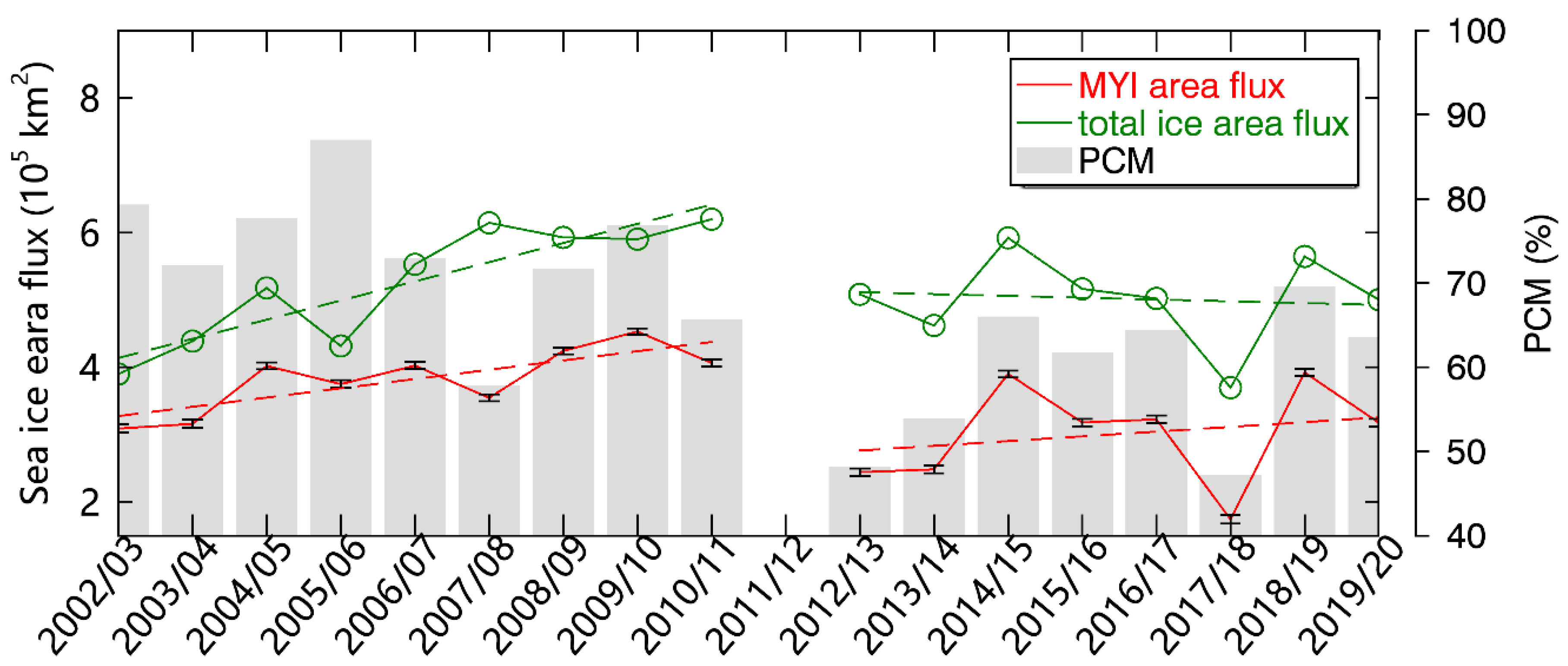
Figure 1. Location of the FS is marked by the red bold line. The studied area comprises a gate connecting point A (11°W, 81.7°N) of Greenland and point B (10.1°E, 79.7°N) of Svalbard.
Remotesensing 14 02562 g001
Figure 2. Sea ice area exports through the FS in winter seasons. The area export variability in MYI (total sea ice) is marked by red (green) lines. Gray bars show the PCM. MYI observations cover October 2002 to April 2020 except for the wintertime of 2011/2012 because of the gap in the operational periods between AMSR-E and AMSR2. The uncertainties of area flux are marked on red line.
Remotesensing 14 02562 g002
Figure 3. The seasonal cycle of MYI (a,b) and total sea ice (d,e) area export through the FS in D1 and D2. PCMs in D1 and D2 are reflected in (g) and (h) respectively. Differences between ice exports in two periods are displayed in the last column of panels (c,f,i).
Remotesensing 14 02562 g003
Figure 4. Monthly variability in the MYI area export anomaly through the FS in winter and spatial patterns of Arctic MYI concentration and sea ice drift corresponding to most four positive/negative events of MYI exports. (a) Top/bottom graphs superimposed by MYI concentration and sea ice drift show the four most positive (MI > 1.4) and negative (MI < −1.8) events for period D1. (b) Top/bottom graphs show four most positive (MI > 1.6) and negative (MI < −1.4) events in period D2. MI is normalized MYI export index and calculated by Equation (5).
Remotesensing 14 02562 g004
Figure 5. Correlation between Mean area of MYI cover in the Arctic ocean and MYI export via FS for winter seasons. (a) Mean Arctic MYI area. The red (black) line indicates 15% (50%) as a cutoff for the lowest MYI concentration to obtain the Arctic MYI area. The MYI area trends during D1 are significant at the 95% confidence level, whereas the trends are not significant during D2. (b) Correlations as a function of lead and lag months between monthly MYI area export and Arctic MYI area anomalies. The blue circles represent confidence levels above 95%. Negative lags represent the MYI area export lagging.
Remotesensing 14 02562 g005
Figure 6. Scatter plots of weekly observations between (a) MYI area export through the FS and MYI concentration across the strait and between (b) MYI area export and gate-perpendicular SIM for the 2002/03–2019/20 period except for 2011/12. The black line represents the linear regression between two variables. Red dashed lines represent 95% deviations, denoting the difference between original data and predicted data. The purple dashed lines indicate 95% confidence bounds of the regression. Above each panel, T is the slope of regression, R is the correlation coefficient. Trends and correlations are all significant at the 99% confidence level.
Remotesensing 14 02562 g006
Figure 7. Wintertime composites of MYI concentration (shaded), SIM (vectors), and SLP (contours) during (a) D1 and (b) D2. The difference between those fields in D1 and D2 is indicated in (c). The unit of SLP is 105 Pa in (a,b), and Pa in (c). The red contours represent positive SLP anomalies, blue contours represent negative anomalies, and yellow contours represent SLP with no difference in (c).
Remotesensing 14 02562 g007
Figure 8. Linkages between MYI export and large-scale atmospheric circulation. (a) Correlations as a function of lag months between monthly MYI area export anomalies the indices of DA, AO, and NAO. The black circle represents confidence levels above 95%. Negative lags represent the MYI area export lagging. (b) The eigenvectors of the second modes of monthly mean SLP north of 70°N in winter during D1 and D2, accounting for 21% and 13% of the total variance, respectively.
Remotesensing 14 02562 g008
Figure 9. The winter pattern of CAI in the Arctic during (a) D1 and (b) D2. (c) Normalized value of the difference between (b,c). Note that the values over Greenland may not be accurate because defining cyclone activity at altitudes higher than 1000 m may not be realistic.
Remotesensing 14 02562 g009
Table 1. The mean (M) and trend (T) in ice exports corresponding to Figure 2.
D1 (2002/03–2010/11)D2 (2012/13–2019/20)All (2002/03–2019/20)Comparison
Mean1
(105 km2)
Trend1
(105 km2/yr)
Mean2
(105 km2)
Trend2
(105 km2/yr)
Mean
(105 km2)
Trend
(105 km2/yr)
(Mean2 − Mean1)/Mean2 (%)
MYI3.82 ± 0.480.143.00 ± 0.75--3.44 ± 0.73--−22
Total ice5.28 ± 0.870.285.02 ± 0.67--5.15 ± 0.77--−5
PCM72%--59%--67%−1.3%/yr
Note: we only show the trend values with significance at a 95% confidence level or higher.
Table 2. Monthly MYI area export through the FS (104 km2).
YearOctoberNovemberDecemberJanuaryFebruaryMarchAprilSum
2002/031.961.341.656.823.6910.185.2330.89
2003/043.352.927.465.886.333.062.5931.58
2004/052.497.528.596.105.156.294.0540.19
2005/066.938.103.331.437.857.562.2937.49
2006/076.888.625.436.142.885.105.1940.24
2007/087.536.495.265.133.414.263.3735.45
2008/094.337.115.575.046.617.945.8242.42
2009/108.756.126.976.414.747.454.8545.30
2010/119.505.145.876.260.957.875.0740.64
Mean5.755.935.575.474.626.644.2738.24
S.D.2.772.422.101.622.132.191.2614.49
2012/136.054.953.891.821.784.021.8924.41
2013/143.497.374.350.902.212.603.9024.82
2014/154.523.2612.123.426.516.013.1739.00
2015/161.536.197.232.535.444.834.0531.79
2016/173.133.206.185.621.647.584.9032.25
2017/182.924.693.162.111.191.851.4617.39
2018/193.295.775.886.125.809.303.0539.22
2019/203.272.213.612.736.839.313.7731.75
Mean3.534.715.803.163.935.693.2730.08
S.D.1.311.732.921.832.432.871.1414.23
Note: Bottom rows give the monthly means and standard deviations (S.D.) of MYI area export during D1 and D2, respectively. The column on the right gives the sum over all winter months in a given year.
Publisher’s Note: MDPI stays neutral with regard to jurisdictional claims in published maps and institutional affiliations.

