Article

Measuring PM2.5 Concentrations from a Single Smartphone Photograph

1
Department of Geography and Resources Management, The Chinese University of Hong Kong, Hong Kong, China
2
Institute of Space and Earth Information Science, The Chinese University of Hong Kong, Hong Kong, China
3
Shenzhen Research Institute, Chinese University of Hong Kong, Hong Kong, China
*
Author to whom correspondence should be addressed.
These authors contributed equally to this work.
Remote Sens. 2022, 14(11), 2572; https://doi.org/10.3390/rs14112572
Submission received: 21 April 2022 / Revised: 19 May 2022 / Accepted: 25 May 2022 / Published: 27 May 2022

Abstract

:
PM2.5 participates in light scattering, leading to degraded outdoor views, which forms the basis for estimating PM2.5 from photographs. This paper devises an algorithm to estimate PM2.5 concentrations by extracting visual cues and atmospheric indices from a single photograph. While air quality measurements in the context of complex urban scenes are particularly challenging, when only a single atmospheric index or cue is given, each one can reinforce others to yield a more robust estimator. Therefore, we selected an appropriate atmospheric index in various outdoor scenes to identify reasonable cue combinations for measuring PM2.5. A PM2.5 dataset (PhotoPM-daytime) was built and used to evaluate performance and validate efficacy of cue combinations. Furthermore, a city-wide experiment was conducted using photographs crawled from the Internet to demonstrate the applicability of the algorithm in large-area PM2.5 monitoring. Results show that smartphones equipped with the developed method could potentially be used as PM2.5 sensors.

Graphical Abstract

1. Introduction

Air pollution has been affecting every inhabited region across the globe, becoming the greatest environmental risk to public health. Globally, approximately 4.2 million premature deaths per year occur due to ambient air pollution [1], and premature mortality arises from exposure to fine particulate matter (PM2.5) [2,3]. Therefore, it is very essential to rapidly and accurately determine ambient PM2.5 concentrations.
Typically, concentrations of PM2.5 measured at fixed air quality monitoring sites [4] are the ideal source of data. However, the extremely sparsely distributed monitoring sites, in addition to the occasional missing values, pose great challenges to applications that require fine-grained PM2.5 data over space and time. Accordingly, many studies have been working on designing new paradigms for air quality measurements [5], such as low-cost devices [6], satellite imageries [7,8], or photographs [9,10]. Among them, photographs have gained particularly great attention because of the ubiquitous use of smartphones and the strong potential for environmental monitoring in near-real time.
Some studies have been conducted to explore the use of photographs as one type of low-cost sensor for air quality monitoring [11,12]. These studies typically rely on the observation that impaired outdoor scenery is the result of the scattering of light by particulates, which forms the basis of measurements. The methods employed by these studies can be broadly classified into two major categories: landscape variation-based and atmospheric optics-based. Landscape variation-based methods directly model the relationship between air quality level changes and variations in landscape characteristics with the requirements of reference information (e.g., registered 3D information [12], obtained substrate photographs [13]). Therefore, they can handle only fixed scenarios. The approaches based on atmospheric optics, as reference-free methods, have become particularly prominent in environmental monitoring in many practical applications [11,14,15]. Atmospheric optics-based approaches generally extract the physical properties of atmospheric scattering from an image-understanding perspective. These physical properties of the atmosphere (i.e., environmental illumination [air-light], the degrading process of luminance flux [transmission], and the attenuation rate of light [extinction]) are estimated on the basis of a standard haze model [16]. Works to date have been developed that move beyond reliance on reference information [9,11], by exploiting fundamental optical models. More recently, the dark channel prior (DCP) method [17] has received a great deal of attention in numerous studies. These methods include the hybrid method based on image processing techniques [18], deep learning-based methods [10,19], or distribution-based methods [11].
As a number of authors have noted, the environmental sensing issued by image understanding frameworks that rely on the extraction of higher-stage features (transmission, extinction) expresses uncertainty over varying scene structures, illuminance levels, and/or albedo of the object’s surface [12,20]. In light of the aforementioned influential factors, most studies treat these as being invariant, rather than as a source of cues to understand environmental change. As suggested in studies of human perception [21] and other photographic-based sensing tasks (e.g., depth estimation, 3D shape determination) [22] a combination of cues can reliably provide strong indicators. Therefore, this cue combination method should be considered in environmental perception. Furthermore, the focus in existing studies on site-specific estimations, limits their operational utility to provide consistent estimations across multiple locations. Therefore, an efficient approach to photograph-based PM2.5 estimation is required for the environmental monitoring of multiple outdoor scenes.
In this paper, we propose an image understanding-based approach for estimating PM2.5 concentrations from smartphone photographs by implementing a combination of atmospheric indices (i.e., local transmission index [LTI] and local extinction index [LEI]) retrieved from photographs and weak cues (i.e., sky discoloration, luminance gradients, and structural information loss) that are extracted from different portions of photographs. Three weak cues are first extracted from the input photograph. Two atmospheric indices are also derived from a series of low-level features and in combination with the DCP method. As weak cues and atmospheric indices are sensitive to the scene structure, we also propose a scene structure-based selection criterion for selecting the appropriate combinations of cues to accurately estimate PM2.5 concentrations.

2. Materials and Methods

Inferring PM2.5 concentrations from a single smartphone photograph is challenging; some photographs may have enough information for reasonable estimates, while other photographs are partially informative or even uninformative. Nevertheless, humans can easily distinguish the ambient environment by looking at different portions of outdoor scenarios for cues, deriving higher levels of visual perception, and manipulating the combination of cues at different levels (e.g., color, contrast at low levels; texture at medium levels; the perception of haze intensity, which is the analog of transmission at high levels) under distinct scenarios (i.e., open and obscured views) [22,23,24]. Inspired by the hierarchical organization and integration mechanism of cues in the human visual system, we propose a hierarchical structural algorithm, whereby the integration of low-level cues and higher-level optical features is considered in the face of various scenarios. Each cue signals different aspects of information, and an appropriate combination of various cues can reinforce the capability of inferring PM2.5 concentrations.

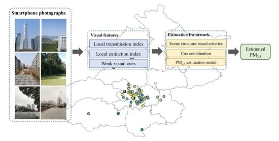
2.1. Weak Cues from a Single Smartphone Photograph

2.1.1. Sky Discoloration

Sky discoloration, which is the difference between the color of the sky region in the given smartphone photograph and an empirical standard color value (i.e., average color intensities of the sky region of photographs captured under good weather). The sky discoloration can be measured using the magnitude of the color gradient in the HSI color space as follows:
H S I s k y = Δ H 2 + Δ S 2 + Δ I 2 ,
where Δ H , Δ S , and Δ I are the hue, saturation, and intensity differences between the sky patch and the empirical standard color. The empirical standard color values of the sky are 3.7207, 0.4675, and 0.5374 (see Supplementary Information Section S1 for details of sky separation and Figure S1).

2.1.2. Luminance Gradients

The luminance of objects results from not only the reflection of sunlight but also the light scattered through the atmosphere onto their surfaces. When haze or smog is dense, the luminance of objects in visual scenes tends to be homogeneous. This phenomenon is described as a “darkness enhancement”, that is, brightness reduction and the enhancement of the darkness of an object [25]. Therefore, the luminance I of each pixel and the variations in the luminance of the photographs are rich information, and this information is the indicator of change in environmental conditions. However, it can be unstable when the surfaces of objects have significant impacts on reflections and when there are obvious variations in lighting conditions [14,26]. Among these influencing factors, the effects of the material properties of object surfaces determine the way in which light is reflected by objects, which strongly interacts with the perception of color and lightness. For objects with a smooth surface (e.g., mirrored architecture, building facades), hereinafter named non-Lambertian regions, specular reflection is dominant and leads to high-frequency spatial distributions and color variations [27]. The significant outliers fused into the luminance information of outdoor scenery might lead to critical problems in estimating luminance information.
Considering the obstacles associated with the presence of non-Lambertian regions in photographs, information on luminance should be solely derived from the separated Lambertian regions, i.e., regions that are insensitive to variations in lighting conditions, of the input photograph. Separating Lambertian regions from photographs is typically performed by constructing the pixelwise confidence to be a Lambertian surface from time-series photographs at a fixed location [14]. The confidence of the Lambertian regions of a fixed scenario is estimated by seeking the best linear correlation between the intensity changes in each pixel over time and the variations in sky luminance Lsky. Traditionally, the luminance map can be calculated from the RGB color space using Equation (2), and the probability that pixel ij is Lambertian P i j L can be calculated using the temporal Pearson correlation:
L i j = 0.299 R i j + 0.587 G i j + 0.114 B i j ,
P i j L = P e a r s o n c o r r ( L i j ,   L s k y )
As discussed above, separating Lambertian regions by reasoning the confidence level from photographs relies on multiple photographs at a fixed location, and, therefore, it is very challenging when only one photograph is given. However, we have experimentally found that within a given image, the proportion of the Lambertian surface is strongly correlated with the scene structure. For instance, for photographs with an obscured view, the proportion of non-Lambertian surfaces dominates the scenes, and reflection causes the luminance gradient map to be fused by outliers (Figure S2i); for photographs with an open view (Figure S2ii), the proportion largely decreases. Therefore, we circumvent the problem of Lambertian region separation by making a simple assumption: the luminance information is calculated only from photographs of open views as a cue to describe variations in the ambient environment. We argue that while this assumption does not eliminate the outliers and biases caused by the strong reflections of non-Lambertian regions, the number of errors can be greatly reduced.
Given a smartphone photograph of open and faraway views, the luminance discontinuities are detected by the gradient magnitude on the luminance component with Equations (4)–(6):
G = G x 2 + G y 2 ,
G x = O x I ,   G y = O x T I ,
O x = ( + 1   + 2   + 1   0   0 0 1 2 1 ) ,
where G x and G y are gradients in the horizontal ( x ) and vertical ( y ) directions, respectively. Furthermore, “ ” is the linear convolution operator, and O x is the Sobel operator applied along the horizontal ( x ) direction. The superscript T in Equation (5) is the transpose operation.

2.1.3. Structural Information Loss

Structural information is independent of luminance and is a good descriptor that reflects how air pollution impairs outdoor scenery [28]. Under heavy haze conditions, the contours of objects (e.g., buildings and roads) in photographs are corrupted; therefore, structural information loss is a cue for the presence of particulate matter.
To quantify structural information loss, we have taken inspiration from the work of Yue et al. [9], who proposed that building contours are preserved in the brightness (gray) color channel but are corrupted in the saturation color channel under heavy haze conditions. The differences between the saturation and brightness of buildings in the given photograph serve as a measure of structural information loss. Then, the information loss is calculated from the gradient similarity between the gray map (brightness) and the saturation color channel in a general form of a structural contrast comparison function [9,28].
Q S = 2 × G g × G s + C G g 2 + G s 2 + C ,
where Q S denotes the gradient similarity. G g and G s are the gradient magnitudes of the grayscale image and saturation component of the image in the HSV color space. C 1 is a non-negative constant and is set as 0.001 in this study. The gradient magnitudes are calculated using Equations (4)–(6). The operators in x and y directions of the gradients are given as follows:
O x = ( + 1 / 3   + 1 / 3   + 1 / 3 0   0 0 1 / 3 1 / 3 1 / 3 )   and   O y = O x T ,  
For Q S , a larger value obtained from the given image indicates that more structural information is retained, which suggests lower haze conditions.

2.2. Local Transmission Index

Particulate matter obscures the clarity of the air, making a photograph blurred. This impaired view is a result of the light scattering of environmental illumination by particles during the transmission process. Therefore, a photograph’s level of degradation is often used as a basis for calculating the haze level via the standard haze model [16,29] as follows:
I ( x ) = t ( x ) J ( x ) + ( 1 t ( x ) ) A ,
where I ( x ) and J ( x ) are the observed intensity of the haze image and the scene radiance of a clear scene, and t ( x ) is the scene transmittance in the light of sight. A , environmental illuminance, is assumed to be globally constant.
The local transmission index ( L T I ) is derived by recovering transmission map t from the observed photograph. To do so, we estimate the transmission map using the DCP based on the work by He et al. [17] and as follows:
t ( x ) = 1 min c ( min y Ω ( x ) ( I c ( y ) A * ) ) ,
where t ( x ) is the transmission map, to be estimated, Ω ( x ) is a patch centered at x with a fixed window size ( 5 × 5 ), and c indicates color channel c th . A * , the ambient light, is calculated from the top 0.1% of pixel intensities in the region just above the horizon. Given t ( x ) , L T I can be estimated as follows:
L T I = ( ln ( t ( x ) ) ) n u m b e r   o f   p i x e l s   , w h e r e   t ˜ ( x ) > 0 ,

2.3. Local Extinction Coefficient

Extinction (hereinafter named the extinction index in this study), a measure of the amount of light scattered and absorbed in the atmosphere, is a global constant parameter when the atmosphere is homogeneous. On the basis of the Beer-Lambert law [30], the relationship between transmission map t ( x ) and extinction coefficient β is given as follows:
t ( x ) = e β d ( x ) ,
where d ( x ) is the estimated depth of scene. Following Equation (12), L E I is derived as follows:
L E I = ln ( t ( x ) ) d ( x ) ,
Equation (13) reveals that the L E I can be calculated once the depth map d ( x ) is able to be provided.

2.3.1. Depth Map

The depth map of the photograph can be estimated via the color attenuation prior [31] and is given as follows:
d ( x ) = θ 0 + θ 1 V ( x ) + θ 2 S ( x ) + ϵ ( x ) ,
Here, V ( x ) and S ( x ) are the intensity of the patch in the value and saturation channels in the HSV color space, respectively. θ 0 = 0.121779 , θ 1 = 0.959710 , and θ 2   = −0.780245. Following a Gaussian distribution, ϵ is the random variable.

2.3.2. Scene Segmentation

As discussed above, the extinction index can be estimated from Equation (13) once the depth map is able to be provided. However, deriving the extinction index directly from the estimated depth map will inevitably lead to more noise (i.e., incorrectly estimated depth). To eliminate apparent noise, calculating these features from a series of large blocks of photographs (i.e., segmented buildings) would be useful [12,32].
The scene in our study is segmented into several parts using three task features (2D segmentation, 2.5D segmentation, and surface norm) from Taskonomy [33]. These three task features from Taskonomy are rescaled to 256 × 256 . Then, a standard upscale operation (bilinear interpolation) is followed to ensure that the resolution of these features is compatible with the other visual cues in this study.

2.3.3. Refined Local Extinction Index

As discussed above, it is suggested that the extinction index be calculated from each segmented object, in combination with Equation (13). This estimation scheme implicitly assumes that the observed illuminance of buildings is not unaffected by surface reflectance; however, this assumption is easily violated in dense urban scenes. For example, a brightly lit surface might not result from higher air-light but may also be associated with building surface reflectance. This phenomenon is referred to as air-light-albedo ambiguity, although it can be reduced by assuming that scene transmission and surface shading are locally uncorrelated [34]. Nevertheless, the disparity illuminance existing within one segmented object and the significant surface reflection of buildings (Figure S3) made by the sun-glint in the photograph make this solution inadequate when large objects (buildings) account for a great proportion of scenes.
To eliminate the uncertainties arising from this problem, we assume that building surface reflectance and albedos are piecewise constant and locally constant in each segmented object [35]. The albedos of surfaces are either known or equal, neither of which is true in real-world applications. However, we have experimentally found that the albedos of vertical objects are often relatively similar within a given photograph, which coincides with a previous study [35]. The albedo differences between direct sun glint and non-direct sun glint regions are also similar. Then, we experimentally found that the highest 1% intensity of each segmented object can be safely considered the result of direct sun glint (for further details, see the Supplementary Information Section S2), and should therefore be removed. Finally, the refined local extinction index can be calculated by rewriting Equation (13).
L E I = ln ( t * ( O ( x ) ) ) d ( O ( x ) ) ,
where O(x) indicates the region of a segmented object, t * ( O ( x ) ) is the transmission of the segmented object after removing the top 1% intensities and d ( O ( x ) ) is the estimated depth for the segmented object.

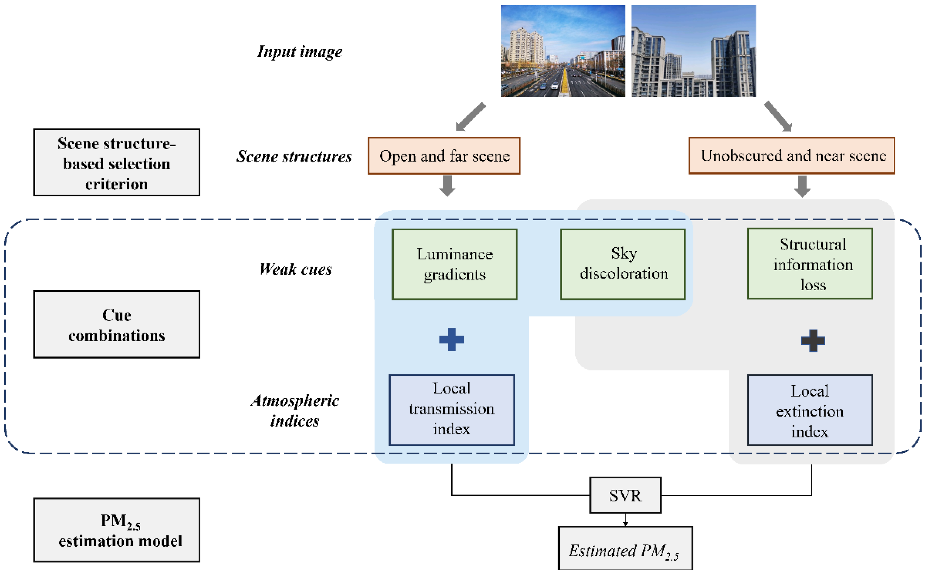
2.4. PM2.5 Estimation Framework

Figure 1 represents the framework of the proposed PM2.5 estimation framework based on the cue combination scheme. Given a smartphone photograph, the general scene categories (open or obscured view) and the appropriate atmospheric index are first determined on the basis of the proposed scene structure-based selection criterion. Then, weak cues reflecting different information of the ambient environment are selected and combined with the selected atmospheric index to give reasonable PM2.5 estimates using support vector regression (SVR).

2.4.1. Scene Structure-Based Selection Criterion

The scene geometric structure of outdoor scenery affects the selection of the appropriate atmospheric index, shapes the combination of cues, and further influences the PM2.5 estimation. The usual explanation is that the LTI derived from the transmission map always assumes that the view is of continuous transition from the scene point to the observer. We take this assumption as indicating that the LTI should be adopted in an open-view scenario because doing so will increase the accuracy of the light attenuation represented in the transmission map, and reduce the uncertainty caused by the presence of large building blocks (such as building surfaces and other objects that compose the scenes). Instead, the LEI, calculated from each building block, is necessary to complement the limits of the transmission map, which provides another explanation for the need for a selection criterion for the scene structure.
The scene structure of an image can be described by low-level features, such as a vanishing point (VP). VPs provide strong information for inferring the spatial arrangement of the main scene structures of an image. In this case, VPs are estimated by RANSAC-based VP detection algorithms [36]. Based on the detected VPs (Figure S4), the criteria for selecting the appropriate atmospheric index can be summarized as follows:
  • For an obscured view, where the VPs are located outside the photograph or are located on objects, and objects (i.e., buildings) dominate the photograph, the local extinction index [LEI] should be selected.
  • For an open view, where the VPs are located far away, typically near the horizon, the local transmission index [LTI] should be selected.

2.4.2. Cue Combination

Previous studies have suggested that cue combinations go beyond the optimization of a single cue because different visual cues indicate information about diverse aspects of the same scene [22,35]. The considerations of cue combinations can help promote effective estimation. Therefore, we propose a cue combination framework that allows each cue to signal different aspects of information in a scene, and the interactions between various cues should enhance their representative performance for PM2.5 estimations.
We summarize the cue combination as follows. In faraway and open scenes, the transmission index is combined with two weak cues (sky distortion and luminance gradient) to jointly infer the environment, namely, LTI-combination. The transmission index from the transmission map is a strong cue for estimating PM2.5, as it is amalgamation information that describes how light is scattered along the light path and is associated with several basic pieces of atmospheric information (e.g., air-light). However, on an overcast day, the air-light can be high because the sky and near horizon will be white, making the estimated transmission map brighter or denser than on sunny days. Therefore, rather than considering the transmission index alone, sky distortion should be considered a complementary cue. Meanwhile, the luminance gradient of the scene is a good descriptor of the variations in views. In contrast, in the case of near and unobscured scenes, the extinction index cooperates with sky distortion and structural information loss to estimate the environmental conditions, namely, the LEI-combination. For example, when a photograph is taken on a sunny day but is backlit, the task of PM2.5 estimation may encounter great problems when solely considering the extinction calculated from objects, because the estimated extinction from building regions will be higher than their vicinity, thus, misestimating the actual level of air quality. This phenomenon proves that, similarly, we should consider ancillary cues. Considering that the estimation of the extinction index is based on the areas of objects, structural information is employed, since such depth-free cues describe only local variations (gradients) in the objects.

2.4.3. PM2.5 Estimation Model

SVR [37] is employed to model the nonlinear relationship between PM2.5 concentrations and the atmospheric index combination:
min ω ,   b 1 2 ω 2 + c i = 1 m ϵ ( ( ω T x i + b ) y i ) ,
where x i is a feature vector and y i is the ground-truth PM2.5 concentration of the i th photograph, ω is the normal vector that determines the direction of the hyperplane, and b is the displacement that determines the distance from the hyperplane to the origin. ϵ represents the ϵ -insensitive loss function, ϵ = 0.1 . In this study, SVR is employed with a radial basis function kernel, e | x y | 2 .

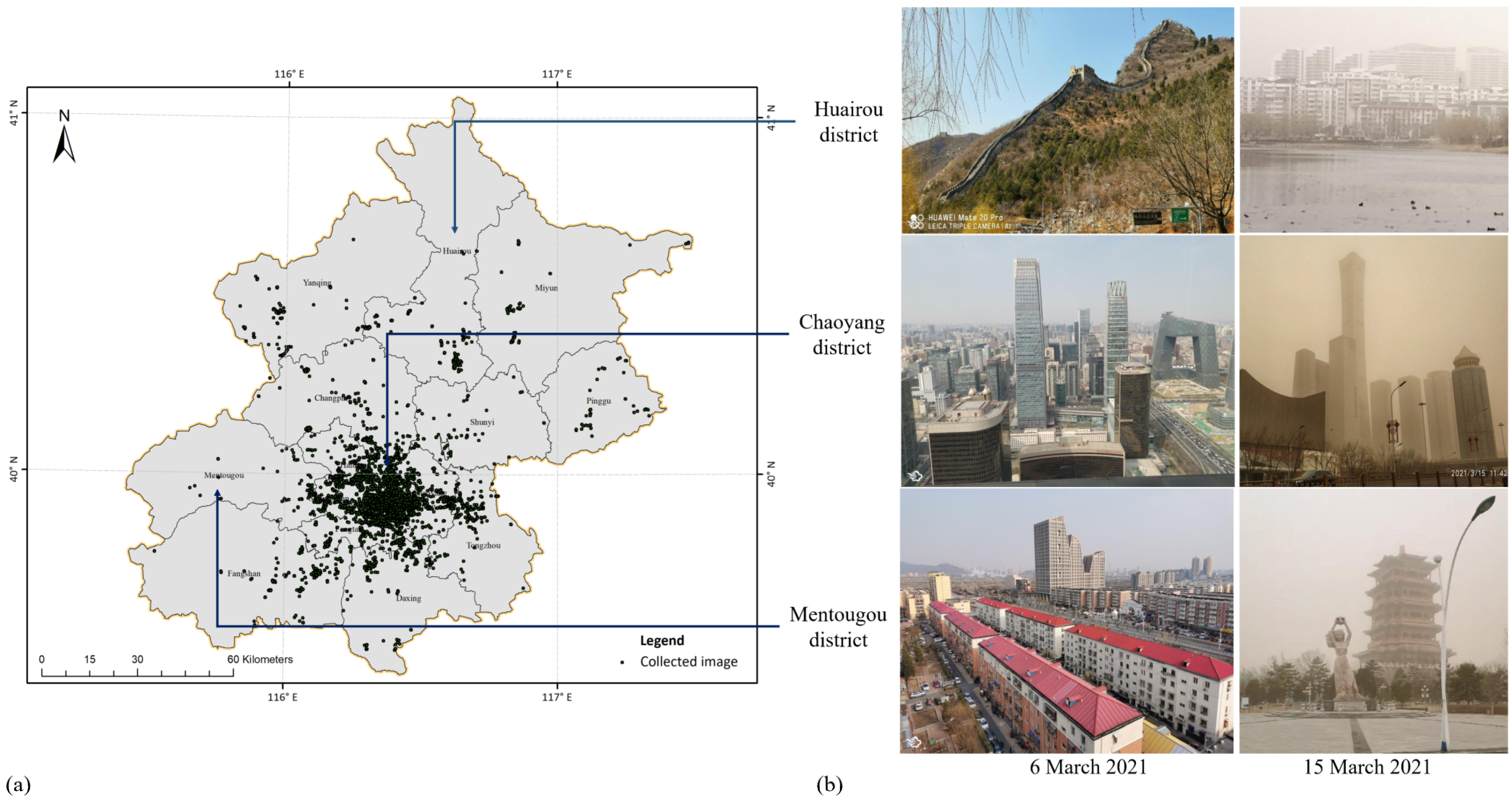
2.5. Experimental Data

2.5.1. PhotoPM-Daytime Dataset

There is no publicly available multi-scenario photograph dataset for local photograph-based PM2.5 concentration estimation; therefore, we first established a specific multi-scenario dataset, namely, PhotoPM-daytime, for estimating PM2.5 concentrations based on smartphone photographs. This dataset involves a total of 2945 photographs that were collected from different locations under different weather conditions, and the photographs contain different scenarios, such as dense urban scenes, lakes, and mountains. Notably, photographs containing rain and snow were excluded. Since these photographs were taken from different smartphones, they have a wide range of photograph resolutions, from 800 × 1200 to 3024 × 4032 . For each photograph, the corresponding PM2.5 concentration value was measured by low-cost portable micro-air quality sensors called “Nature Clean” (Nature Clean AM-300; http://www.aiqiworld.com/topic_1049.html (accessed on 13 May 2022)). This low-cost monitor measures the concentrations of local ambient air quality through an embedded light scattering laser sensor and Table S2 lists the specifications of this portable sensor. The number of photographs taken at different levels of PM2.5 concentration for the PhotoPM-daytime dataset is presented in Figure 2.

2.5.2. Crowdsourced Photographs from the Internet

Photographs were crowdsourced from the “Moji Weather” application, a weather-centered social media platform on which users post pictures tagged with geolocations. We used the crawling technique to collect photographs posted by users in Beijing. A total of 11,059 photographs, from 1 March 2021 to 31 March 2021, were collected (Figure 3). The profile of each record includes username, the timestamp of the photograph, and the associated location (toponym, GPS coordinates) where the photograph was taken.

3. Results

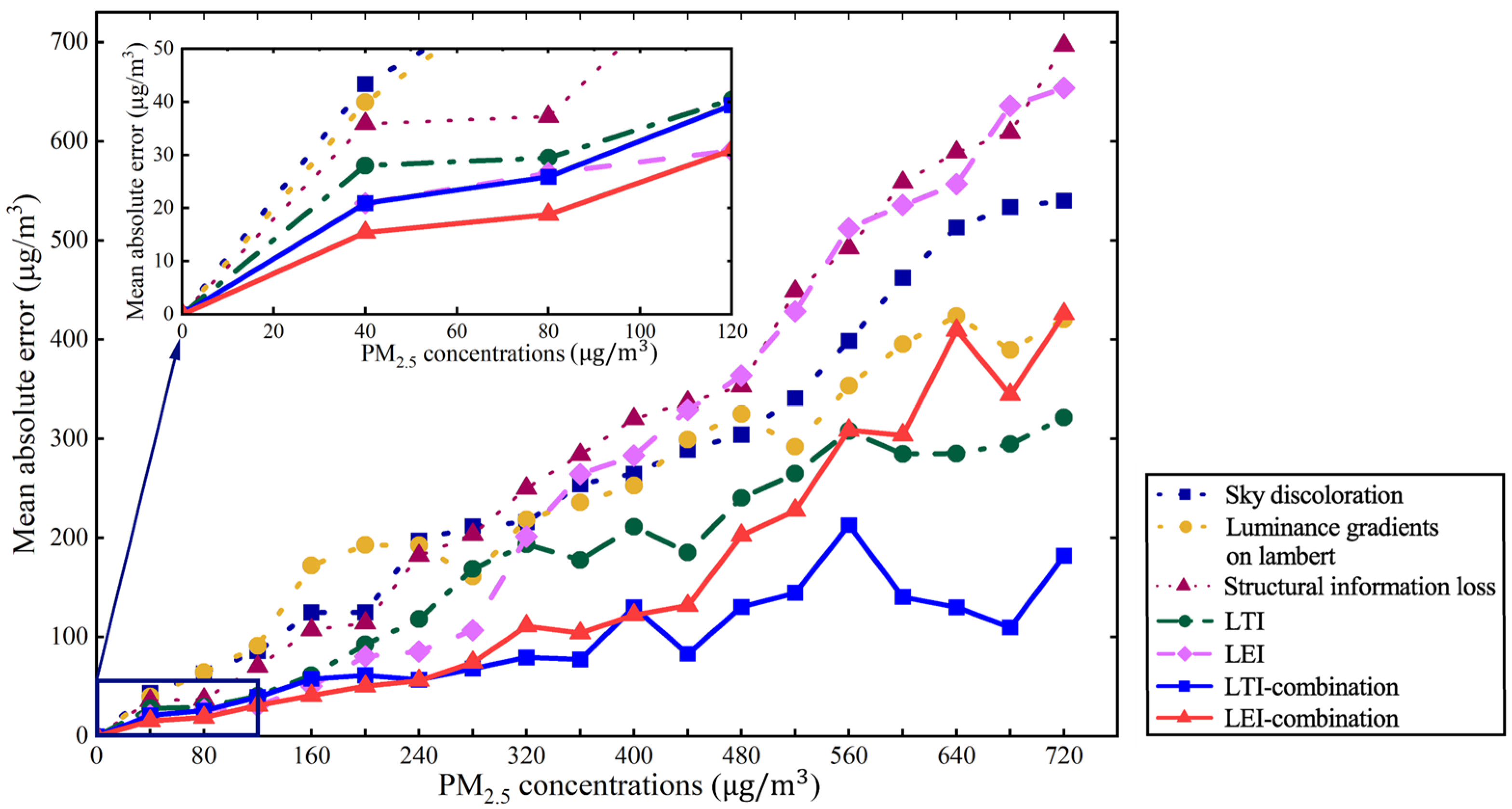
3.1. Evaluation of the Cue Combinations for PM2.5 Estimation

To evaluate the reliability and benefits of cue combinations for single cues, cues and their combinations in the proposed algorithm were applied to the photoPM-daytime dataset independently. They thus formed seven scenarios: using only weak cues, using optical features only (LTI and LEI), and using combined measures, LTI-combination and LEI-combination. In each scenario, the single cue, or cue combination, was fitted to the PM2.5 concentrations using the SVR model, and the estimated concentrations were compared against the ground truth.
Figure 4 illustrates the mean absolute errors (MAEs) of PM2.5 estimation for different scenarios. The errors in estimates from each scenario varied independently. In general, the results showed that two cue combinations (the last two curves: the red and royal blue curve for LEI-combination and LTI-combination, respectively) that combined weak cues and optical features apparently had stronger informative power and promoted more effective PM2.5 estimations. This superiority of the cue combinations, compared to single cues (either weak cues or atmospheric indices), was consistent across the whole range of air pollution. Two atmospheric indices, LTI and LEI (as shown in the green and pink dashed curves, respectively), appeared to obtain fairly reliable estimates when compared to weak cues, indicating their power in interpreting the ambient environment; however, they may be prone to extreme outlier estimates under complex conditions.
Moreover, the disparities in compensatory improvements (performance improvements resulting from the combination of cues) were significant, indicating that cues differently contribute to the end result at different levels of air pollution. For instance, structural information loss promotes LEI performance by disambiguating the sign of different building regions in regions having relatively slight air pollution (lower than approximately 120 μg/m3); in contrast, sky discoloration partially promotes LEI performance under heavy haze conditions (see the difference between the LEI and the sky discoloration). The luminance gradient greatly affects the estimation power of LTI-combination under heavy haze conditions (greater than approximately 480 μ g / m 3 ).
To summarize, the quantitative comparisons in Figure 4 show strong support for the improved performance in air quality estimation in light of the cue combination. However, there were also cases in which a less effective approach resulted in larger errors, e.g., when LEI-combination was applied to photographs that were taken under heavy haze. Ambiguity in interpreting the scene structure under heavy haze is the major problem leading to extreme outliers, which could be reduced by the proposed selection criterion and will be discussed shortly.

3.2. Validation of the PM2.5 Estimation Model

3.2.1. Performance of the Estimation Model

To verify the effectiveness of the proposed algorithm in general and dynamic outdoor scenarios, a 5-fold cross-validation (CV) was conducted. A Python tool was coded for this purpose. Figure 5 shows the scatterplots of the CV results. Figure S5 shows examples of photographs with their estimated PM2.5 concentrations.
The CV R2 values of the two atmospheric index combinations were 0.779 and 0.572 for the LTI and LEI coefficients, respectively, and the RMSE values were 61.998 and 87.136 μg/m3, respectively. As expected, the CV results with a selected atmospheric index exhibited overwhelming superiority compared to those obtained by the models using only one atmospheric index; the R2 value increased by 0.073 and 0.280, and the RMSE values decreased by 11.475 and 36.613 μg/m3. The validation results proved that considering the scene structures in models can strongly increase prediction accuracy.

3.2.2. Performance under Different Outdoor Sceneries

The scene structure (including the layout and geometry of photographs) impacted the accuracy of the estimation results by affecting the performance of atmospheric index and weak cue extraction. Therefore, exploring the model performance in different scenarios is essential to understand the sensitivity associated with scene structures. To verify the effectiveness of the PM2.5 estimation algorithm in different typical scenarios, we first classified the PhotoPM-daytime dataset into two major categories: natural environments and man-made environments, following the image classification standard of the SUN database [38]. The R 2 and RMSE were used to evaluate the models in different outdoor scene categories. Figure S6 shows the sample photographs of each scene category. A detailed description of each subcategory is given in Supplemental Table S3.
Table 1 summarizes the estimation results of the model in different outdoor scenarios in terms of the R 2 and RMSE values for L T I -combination, L E I -combination, and a selected atmospheric index combination. Generally, the results suggest that the selected atmospheric index combination consistently achieved a good performance under outdoor man-made and outdoor natural conditions over L T I -combination and L E I -combination, in terms of the higher R 2 values and lower RMSE values. Notably the estimation accuracy of the selected atmospheric index combination exhibited significant disparities under diverse outdoor scenarios.
Specifically, in an outdoor man-made environment, the selected atmospheric index combination showed a consistently good performance for three categories (C1–C3), in terms of the high R 2 and low RMSE values (the R 2 values were all above 0.830, and the RMSE values were all below 64.420   μ g / m 3 ). Notably the selected combination displayed the greatest performance in C3 (buildings), the most complex urban scenes, with an R 2 value reaching 0.872 and an RMSE value of only 58.112 μ g / m 3 . This good performance was also remarkable in C2 (leisure spaces), for which the selected combination outperformed L T I -combination and L E I -combination by 16.54% and 47.85%, in terms of the RMSE values (from 57.110 and 91.582 to 47.761   μ g / m 3 ).
Unlike the aforementioned scenarios, the proposed algorithm did not show remarkably precise estimates for outdoor natural scenes. From the results in Table 1, we note that the best performance under the outdoor natural categories was obtained in the category of man-made elements (C6: R 2   = 0.789; RMSE = 39.239 μ g / m 3 ). The lowest performance was found in C4 and C5, with goodness of fit values of only 0.669 and 0.678, respectively. Although the estimation performance shows inferiority to the other categories, considering the comparable goodness of fit ( R 2 value greater than 0.670) and the complex scenarios of the photographs, the results still proved the validity of the model. One possible reason for this inferiority in C1 (water) is that the water content and reflected light intensities reflect scene illumination, generate higher atmospheric light values, and thus involve air-light-luminance ambiguity. For C5, the reflection and absorption effects are different from the majority of urban scenarios; independent considerations of a single-color channel have been shown to improve certain types of performance, as discussed in [12,39]. In this study, we did not consider them to be a special case, because the objective was to generate algorithms that are capable of handling multiple views.
Therefore, these results indicate that the selected atmospheric index combination provides reasonable and accurate estimates by selecting an appropriate combination, highlighting the applicability of the estimates to highly complex situations in dense urban scenarios.

3.3. PM2.5 Estimation for Beijing

Figure 6 presents maps of the estimated PM2.5 concentrations using the proposed algorithm at four time slots (7:00 am and 8:00 am on 15 March 2021 and 10:00 am and 11:00 am on 29 March 2021). It should be noted that the present distribution (Figure 6) only involved the estimations in central Beijing for a better visual effect, as the majority of collected photographs are concentrated there (Figure 3).
Generally, the PM2.5 values of the crowdsourced photographs exhibited a remarkable spatiotemporal heterogeneity. Specifically, on 15 March 2021, which was a day that a mega sand and dust storm event occurred, and the average PM2.5 concentrations at 7:00 am and 8:00 am were 220.775 and 586.678 μg/m3, respectively. At 8:00 am (Figure 6b), the estimated distribution pattern exhibited a strong heterogeneity over space. The PM2.5 concentrations in northern and central Beijing were significantly higher than those in southern Beijing, showing a significant decreasing trend from the city’s northwest to southeast regions. However, this spatial heterogeneity was inconspicuous at 7:00 am. These disparities across space and time revealed that the dust transport process was strongly associated with the meteorological factor (mainly driven by north-westerly winds) and had a high magnitude, which is in accordance with the results of previous studies [40]. Moreover, on 29 March (average estimated PM2.5 was 23.673 μ g / m 3 ) (Figure 6c,d), a limited heterogeneity was observed, suggesting relatively homogeneous air quality patterns. We can infer from these results that, by employing the proposed algorithm, the smartphone photographs could be turned into low-cost and mobile sensors which are spatially denser than monitoring stations. Furthermore, the proposed photograph-based PM2.5 concentration measurement holds great potential to be a reliable alternative for monitoring ambient air pollutants.

4. Discussion

4.1. Comparison with Other Methods Using the PhotoPM-Daytime Dataset

To make comparisons, we compared the performance of the proposed algorithm, based on the PhotoPM-daytime dataset, with the specialized PM2.5 estimation techniques of Rijal et al. [19], Jian et al. [18], and Gu et al. [11]. Among them, Rijal et al. [19] and Jian et al. [18] used deep learning-based techniques. In contrast, the algorithm of Gu et al. [11] was distribution based, where the distribution is built on entropy features extracted using image analysis techniques. The results of Rijal et al. [19] and Jian et al. [18] were obtained from models that we implemented ourselves according to the reported procedures in the articles, and the results of Gu et al. [11] were derived from the provided source code.
Table 2 summarizes the comparison results among the methods described above in terms of the MAE, RMSE, and Pearson correlation (Pearson r). The results of our algorithm are given in the last line of the table. Table 2 shows that the obtained results improved upon those of the state-of-the-art methods. In particular, we observed that the proposed algorithm outperformed the two deep learning-based algorithms in terms of decreased RMSE and MAE values (15.303 and 40.364 μ g / m 3 ; 27.242 and 35.196 μ g / m 3 for Rijal et al. [19] and Jian et al. [18], respectively). Considering the complexity of the PhotoPM-daytime dataset and the high variability, due to the diverse outdoor scenarios, the reduction in the RMSE value of 40.364 μ g / m 3 can be considered a remarkable improvement, indicating that the proposed image analysis-based algorithm has an excellent capability over these deep learning-based algorithms due to the appropriate combination of cues. Surprisingly, we found that, compared to Gu et al. (2019), the proposed algorithm displayed a better performance by decreasing the RMSE and MAE values by 68.529% and 56.613%, respectively, and by increasing the Pearson r by 0.686. One possible reason for this result might be that the algorithm of Gu et al. [11] estimated PM2.5 concentrations by measuring the likelihood of deviation of the input photographs from “standard” photographs (photographs taken under good weather), indicating that the transferability of the algorithm would be greatly impeded by the selection of “standard” photographs. However, our proposed algorithm can effectively reduce the reliance on preset standards, differing from Gu et al. [11], by considering the joint effects of weak cues (partially relying on preset standards) and atmospheric indices.

4.2. Transferability of the PM2.5 Estimation Model Based on Other Datasets

Generalizability and transferability are important issues for algorithms when applied to real-world applications. Therefore, we also evaluated the proposed algorithms based on two public datasets: the Shanghai-1954 dataset [41,42] and the Beijing-1460 dataset [19]. The Shanghai-1954 dataset consists of 1954 daytime (8:00 am to 16:00 pm) photographs (584 × 389 resolution) with a fixed viewpoint (Oriental Pearl Tower) and the corresponding PM2.5 index (ranging from 0–206) obtained from published documents by the U.S. consulate. The Beijing-1460 dataset has a total of 1460 images (resolution higher than 584 × 389) of different outdoor scenes in Beijing. The corresponding PM2.5 levels for the Shanghai-1954 and Beijing-1460 datasets were measured by the Met One BAM-1020 and collected from the historical data provided by the U.S. Embassy.
Table 3 summarizes the transferability performance of the proposed algorithm in terms of the RMSE, Pearson r, and goodness of fit R2 values based on the two public datasets. As observed, for the Shanghai-1954 dataset, our algorithm showed slightly better performance with respect to the estimation of the PM2.5 index than the others in terms of the increased R2 values of 0.002 (from 0.872 to 0.874), although the increased performance was not as significant as that shown in Section 4.1. Notably, the estimation of the PM index should be regarded as a different task, while our proposed algorithm was specially designed for PM2.5 estimation. Therefore, these slight advantages still provide evidence that the proposed algorithm has transferability that is comparable to that of other datasets and even shows stronger robustness than other specially designed algorithms.
In addition, the superiority of the proposed algorithm was much more obvious compared to the others based on the Beijing-1460 dataset, with the goodness of fit value increasing by 0.064 (from 0.627 to 0.691) and the RMSE values decreasing by 4.611 μ g / m 3 (from 53.63 to 48.969 μ g / m 3 ). The results show that although the estimation accuracy was more precise than other techniques, such superiority was not as significant as initially expected. One possible reason for these results may be a “mismatching” problem because each photo’s PM2.5 values were measured from a fixed location (the U.S. embassy) in Beijing, while the photographs were taken from different locations. Considering that the spatial distribution of PM2.5 values has great variability, a value measured at a fixed location may not be representative of the situation at the place where the photograph was taken, thus inevitably introducing biases. Nevertheless, the performance comparisons based on two public datasets demonstrate that the proposed algorithm has strong transferability and generalizability, and, thus, they further suggest that the proposed algorithm can potentially be applied in various scenarios and achieve high accuracy which will be discussed shortly.

4.3. Limitations and Future Work

Despite these encouraging results, there are some aspects of our methods that could be further improved. First, the proposed method can only be applied to estimate PM2.5 concentrations from smartphone photographs taken during the daytime. As a result, nighttime PM2.5 concentration estimates have not been made available. Another possible restriction of this study is that the PM2.5 distributions of the PhotoPM-daytime dataset are unequally distributed, and, thus, we will continue to collect more smartphone photographs in future studies, especially at high PM2.5 concentrations, to balance the distribution of PM2.5 concentrations and increase the dataset size.

5. Conclusions

This paper presents algorithms for measuring PM2.5 concentrations by extracting atmospheric indices and weak cues from a single photograph. The algorithms were first tested on a PM2.5 image dataset with 2945 photographs taken at different locations under various haze levels. Our approach exploits the “collective wisdom” of cue combinations from these cues to promote more effective estimates. In this way, the presented estimation method can still provide reasonable estimates, even when photographs are partially informative. By considering a photograph’s scene structures, the proposed algorithms can automatically select appropriate atmospheric index combinations. This ability overcomes the weakness of traditional photograph-based methods that are capable for fixed scenes; thus, the proposed algorithms can treat complex and dense urban scenes. In addition, the algorithms show the ability to generalize to other data sources (e.g., photographs from networks) and to transfer to different environmental sensing tasks (e.g., estimation of the PM index from a single photo). Furthermore, an experiment in Beijing was performed, demonstrating the applicability of the proposed algorithm in a real-world scenario and highlighting the potential of smartphones as real-time environmental sensors. Thus, this study demonstrated an efficient and convenient method of measuring PM2.5 concentrations at a significantly low cost. The developed algorithm has the potential to transform ubiquitous smartphones into mobile sensors, which can complement ground monitoring stations and provide citizens with a powerful tool to monitor their ambient air quality.

Supplementary Materials

The following supporting information can be downloaded at: https://www.mdpi.com/article/10.3390/rs14112572/s1, Figure S1: Haze cues from the sky only. Starting from the input photograph (a), we extract the sky regions (b) with the sky probability model. The extracted sky regions in the HSI color space are presented in (c) under two distinct environmental conditions; Figure S2: Examples of photographs (a) transformed luminance maps (b), and luminance gradient maps (c) under two weather conditions, clear and heavy haze conditions, for photographs in which non-Lambertian regions dominate (i) and Lambertian regions dominate (ii); Figure S3: Examples of the direct sun-glint; Figure S4: Detected vanishing points (red dots) in (a) open view photographs and (b) obscured view photographs; Figure S5: Successful (a) and Failed (b) example photographs with their observed and estimated PM2.5 concentrations; Figure S6: Example photographs in each outdoor scene category; Table S1: The measured albedo in two general types of buildings; Table S2: Specifications of the Nature Clean sensor; Table S3: Detailed descriptions of each sub-category [43,44,45,46,47].

Author Contributions

Conceptualization, B.H.; methodology, S.Y. and B.H.; data curation, S.Y. and F.W.; validation, S.Y. and F.W.; formal analysis, S.Y.; writing—original draft preparation, S.Y.; writing—review and editing, S.Y. and B.H.; visualization, S.Y.; supervision, B.H. All authors have read and agreed to the published version of the manuscript.

Funding

This research was funded by the Hong Kong Research Grants Council (CRF C4139-20G and AoE/E-603/18), the Strategic Priority Research Program of the Chinese Academy of Sciences (XDA19090108) and the National Key R&D Program of China (2019YFC1510400 and 2017YFB0503605).

Data Availability Statement

The Shanghai-1954 dataset and the Beijing-1460 dataset can be downloaded at https://figshare.com/articles/figure/Particle_pollution_estimation_based_on_image_analysis/1603556, accessed on 14 February 2022.

Conflicts of Interest

The authors declare no conflict of interest.

References

  1. World Health Organization. Ambient Air Pollution: A Global Assessment of Exposure and Burden of Disease; World Health Organization: Geneva, Switzerland, 2016; ISBN 978-92-4-151135-3.
  2. Song, Y.M.; Huang, B.; He, Q.Q.; Chen, B.; Wei, J.; Rashed, M. Dynamic Assessment of PM2·5 Exposure and Health Risk Using Remote Sensing and Geo-spatial Big Data. Environ. Pollut. 2019, 253, 288–296. [Google Scholar] [CrossRef] [PubMed]
  3. Yue, H.; He, C.; Huang, Q.; Yin, D.; Bryan, B.A. Stronger Policy Required to Substantially Reduce Deaths from PM2.5 Pollution in China. Nat. Commun. 2020, 11, 1462. [Google Scholar] [CrossRef] [PubMed] [Green Version]
  4. Ministry of Ecology and Environment the People’s Republic of China. The State Council Issues Action Plan on Prevention and Control of Air Pollution Introducing Ten Measures to Improve Air Quality. Available online: http://english.mee.gov.cn/News_service/infocus/201309/t20130924_260707.shtml (accessed on 4 January 2021).
  5. Snyder, E.G.; Watkins, T.H.; Solomon, P.A.; Thoma, E.D.; Williams, R.W.; Hagler, G.S.W.; Shelow, D.; Hindin, D.A.; Kilaru, V.J.; Preuss, P.W. The Changing Paradigm of Air Pollution Monitoring. Environ. Sci. Technol. 2013, 47, 11369–11377. [Google Scholar] [CrossRef] [PubMed]
  6. Milà, C.; Salmon, M.; Sanchez, M.; Ambrós, A.; Bhogadi, S.; Sreekanth, V.; Nieuwenhuijsen, M.; Kinra, S.; Marshall, J.D.; Tonne, C. When, Where, and What? Characterizing Personal PM2.5 Exposure in Periurban India by Integrating GPS, Wearable Camera, and Ambient and Personal Monitoring Data. Environ. Sci. Technol. 2018, 52, 13481–13490. [Google Scholar] [CrossRef] [PubMed] [Green Version]
  7. He, Q.; Huang, B. Satellite-Based Mapping of Daily High-Resolution Ground PM2.5 in China via Space-Time Regression Modeling. Remote Sens. Environ. 2018, 206, 72–83. [Google Scholar] [CrossRef]
  8. Fan, W.; Qin, K.; Cui, Y.; Li, D.; Bilal, M. Estimation of Hourly Ground-Level PM2.5 Concentration Based on Himawari-8 Apparent Reflectance. IEEE Trans. Geosci. Remote Sens. 2021, 59, 76–85. [Google Scholar] [CrossRef]
  9. Yue, G.; Gu, K.; Qiao, J. Effective and Efficient Photo-Based PM2.5 Concentration Estimation. IEEE Trans. Instrum. Meas. 2019, 68, 3962–3971. [Google Scholar] [CrossRef]
  10. Zhang, Q.; Fu, F.; Tian, R. A Deep Learning and Image-Based Model for Air Quality Estimation. Sci. Total Environ. 2020, 724, 138178. [Google Scholar] [CrossRef]
  11. Gu, K.; Qiao, J.; Li, X. Highly Efficient Picture-Based Prediction of PM2.5 Concentration. IEEE Trans. Ind. Electron. 2019, 66, 3176–3184. [Google Scholar] [CrossRef]
  12. Pudasaini, B.; Kanaparthi, M.; Scrimgeour, J.; Banerjee, N.; Mondal, S.; Skufca, J.; Dhaniyala, S. Estimating PM2.5 from Photographs. Atmos. Environ. X 2020, 5, 100063. [Google Scholar] [CrossRef]
  13. Liaw, J.-J.; Huang, Y.-F.; Hsieh, C.-H.; Lin, D.-C.; Luo, C.-H. PM2.5 Concentration Estimation Based on Image Processing Schemes and Simple Linear Regression. Sensors 2020, 20, 2423. [Google Scholar] [CrossRef] [PubMed]
  14. Babari, R.; Hautière, N.; Dumont, É.; Paparoditis, N.; Misener, J. Visibility Monitoring Using Conventional Roadside Cameras—Emerging Applications. Transp. Res. Part C Emerg. Technol. 2012, 22, 17–28. [Google Scholar] [CrossRef] [Green Version]
  15. Qin, H.; Qin, H. Image-Based Dedicated Methods of Night Traffic Visibility Estimation. Appl. Sci. 2020, 10, 440. [Google Scholar] [CrossRef] [Green Version]
  16. Koschmieder, H. Theorie Der Horizontalen Sichtweite. Beitr. Zur Phys. Der Freien Atmosphare 1924, 12, 33–53. [Google Scholar]
  17. He, K.; Sun, J.; Tang, X. Single Image Haze Removal Using Dark Channel Prior. IEEE Trans. Pattern Anal. Mach. Intell. 2011, 33, 2341–2353. [Google Scholar]
  18. Jian, M.; Kun, L.; Han, Y.H. Image-based PM2.5 Estimation and its Application on Depth Estimation. In Proceedings of the 2018 IEEE International Conference on Acoustics, Speech and Signal Processing (ICASSP), Calgary, AB, Canada, 15–20 April 2018. [Google Scholar]
  19. Rijal, N.; Gutta, R.T.; Cao, T.; Lin, J.; Bo, Q.; Zhang, J. Ensemble of Deep Neural Networks for Estimating Particulate Matter from Images. In Proceedings of the 2018 IEEE 3rd International Conference on Image, Vision and Computing (ICIVC), Chongqing, China, 27–29 June 2018; pp. 733–738. [Google Scholar]
  20. Eldering, A.; Hall, J.R.; Hussey, K.J.; Cass, G.R. Visibility Model Based on Satellite-Generated Landscape Data. Environ. Sci. Technol. 1996, 30, 361–370. [Google Scholar] [CrossRef]
  21. Groen, I.I.A.; Silson, E.H.; Baker, C.I. Contributions of Low- and High-Level Properties to Neural Processing of Visual Scenes in the Human Brain. Philos. Trans. R. Soc. B Biol. Sci. 2017, 372, 20160102. [Google Scholar] [CrossRef] [Green Version]
  22. Landy, M.S.; Maloney, L.T.; Johnston, E.B.; Young, M. Measurement and Modeling of Depth Cue Combination: In Defense of Weak Fusion. Vis. Res. 1995, 35, 389–412. [Google Scholar] [CrossRef] [Green Version]
  23. Arcaro, M.J.; Honey, C.J.; Mruczek, R.E.; Kastner, S.; Hasson, U. Widespread Correlation Patterns of FMRI Signal across Visual Cortex Reflect Eccentricity Organization. eLife 2015, 4, e03952. [Google Scholar] [CrossRef] [Green Version]
  24. Grill-Spector, K.; Malach, R. The Human Visual Cortex. Annu. Rev. Neurosci. 2004, 27, 649–677. [Google Scholar] [CrossRef] [Green Version]
  25. Zavagno, D. Some New Luminance-Gradient Effects. Perception 1999, 28, 835–838. [Google Scholar] [CrossRef] [PubMed]
  26. Giesel, M.; Gegenfurtner, K.R. Color Appearance of Real Objects Varying in Material, Hue, and Shape. J. Vis. 2010, 10, 10. [Google Scholar] [CrossRef] [PubMed] [Green Version]
  27. Shi, J.; Dong, Y.; Su, H.; Yu, S.X. Learning Non-Lambertian Object Intrinsics Across ShapeNet Categories. In Proceedings of the 2017 IEEE Conference on Computer Vision and Pattern Recognition (CVPR), Honolulu, HI, USA, 21–26 July 2017; pp. 1685–1694. [Google Scholar]
  28. Wang, Z.; Bovik, A.C.; Simoncelli, E.P. Structural Approaches to Image Quality Assessment. In Handbook of Image and Video Processing; Elsevier: Amsterdam, The Netherlands, 2005; pp. 961–974. ISBN 978-0-12-119792-6. [Google Scholar]
  29. Cozman, F.; Krotkov, E. Depth from Scattering. In Proceedings of the IEEE Computer Society Conference on Computer Vision and Pattern Recognition, San Juan, PR, USA, 17–19 June 1997. [Google Scholar]
  30. Swinehart, D.F. The Beer–Lambert Law. J. Chem. Educ. 1962, 39, 3. [Google Scholar] [CrossRef]
  31. Zhu, Q.; Mai, J.; Shao, L. A Fast Single Image Haze Removal Algorithm Using Color Attenuation Prior. IEEE Trans. Image Process. 2015, 24, 3522–3533. [Google Scholar]
  32. Wang, H.; Yuan, X.; Wang, X.; Zhang, Y.; Dai, Q. Real-Time Air Quality Estimation Based on Color Image Processing. In Proceedings of the 2014 IEEE Visual Communications and Image Processing Conference, Valletta, Malta, 7–10 December 2014; pp. 326–329. [Google Scholar]
  33. Zamir, A.R.; Sax, A.; Shen, W.; Guibas, L.; Malik, J.; Savarese, S. Taskonomy: Disentangling Task Transfer Learning. In Proceedings of the IEEE Conference on Computer Vision and Pattern Recognition (CVPR), Salt Lake City, UT, USA, 18–23 June 2018; pp. 3712–3722. [Google Scholar]
  34. Fattal, R. Single Image Dehazing. ACM Trans. Graph. 2008, 27, 1–9. [Google Scholar] [CrossRef]
  35. Lalonde, J.-F.; Efros, A.; Narasimhan, S. Estimating Natural Illumination Conditions from a Single Outdoor Image. Int. J. Comput. Vis. 2012, 98, 123–145. [Google Scholar] [CrossRef]
  36. Chaudhury, K.; DiVerdi, S.; Ioffe, S. Auto-Rectification of User Photos. In Proceedings of the 2014 IEEE International Conference on Image Processing (ICIP), Paris, France, 27–30 October 2014; pp. 3479–3483. [Google Scholar]
  37. Cortes, C.; Vapnik, V. Support-Vector Networks. Mach. Learn. 1995, 20, 273–297. [Google Scholar] [CrossRef]
  38. Xiao, J.; Hays, J.; Ehinger, K.A.; Oliva, A.; Torralba, A. SUN Database: Large-Scale Scene Recognition from Abbey to Zoo. In Proceedings of the 2010 IEEE Computer Society Conference on Computer Vision and Pattern Recognition, San Francisco, CA, USA, 13–18 June 2010; pp. 3485–3492. [Google Scholar]
  39. Larson, S.M.; Cass, G.R.; Hussey, K.J.; Luce, F. Verification of Image Processing Based Visibility Models. Environ. Sci. Technol. 1988, 22, 629–637. [Google Scholar] [CrossRef]
  40. Gui, K.; Yao, W.; Che, H.; An, L.; Zheng, Y.; Li, L.; Zhao, H.; Zhang, L.; Zhong, J.; Wang, Y.; et al. Two Mega Sand and Dust Storm Events over Northern China in March 2021: Transport Processes, Historical Ranking and Meteorological Drivers. Atmos. Chem. Phys. Discuss. 2021; in review. [Google Scholar] [CrossRef]
  41. Bo, Q.; Yang, W.; Rijal, N.; Xie, Y.; Feng, J.; Zhang, J. Particle Pollution Estimation from Images Using Convolutional Neural Network and Weather Features. In Proceedings of the 2018 25th IEEE International Conference on Image Processing (ICIP), Athens, Greece, 7–10 October 2018; pp. 3433–3437. [Google Scholar]
  42. Liu, C.; Tsow, F.; Zou, Y.; Tao, N. Particle Pollution Estimation Based on Image Analysis. PLoS ONE 2016, 11, e0145955. [Google Scholar] [CrossRef]
  43. Rayleigh, L. XXXIV. On the Transmission of Light through an Atmosphere Containing Small Particles in Suspension, and on the Origin of the Blue of the Sky. Lond.Edinb. Dublin Philos. Mag. J. Sci. 1899, 47, 375–384. [Google Scholar] [CrossRef] [Green Version]
  44. Middleton, W.E.K. Vision through the Atmosphere. In Geophysik II/Geophysics II; Bartels, J., Ed.; Handbuch der Physik/Encyclopedia of Physics; Springer: Berlin/Heidelberg, Germany, 1957; pp. 254–287. ISBN 978-3-642-45881-1. [Google Scholar]
  45. Liu, X.; Song, Z.; Ngai, E.; Ma, J.; Wang, W. PM2:5 Monitoring Using Images from Smartphones in Participatory Sensing. In Proceedings of the 2015 IEEE Conference on Computer Communications Workshops (INFOCOM WKSHPS), Hong Kong, 26 April–1 May 2015; pp. 630–635. [Google Scholar]
  46. Solar Light Company Solarmeter. Available online: https://www.solarmeter.com/ (accessed on 18 November 2021).
  47. Lalonde, J.-F.; Efros, A.; Narasimhan, S. Estimating Natural Illumination from a Single Outdoor Image. In Proceedings of the IEEE 12th International Conference on Computer Vision, ICCV 2009, Kyoto, Japan, 27 September–4 October 2009; p. 190. [Google Scholar]
Figure 1. Workflow of the proposed PM2.5 concentration estimation framework.
Remotesensing 14 02572 g001
Figure 2. Number of smartphone photographs taken at different levels of PM2.5 concentration as measured by the “Nature Clean” monitor for the PhotoPM-daytime dataset.
Remotesensing 14 02572 g002
Figure 3. Spatial distribution of photographs crowdsourced from Moji Weather application (a) and example photographs taken at three districts (b).
Remotesensing 14 02572 g003
Figure 4. Performance comparisons of a single cue and cue combinations when estimating PM2.5 concentrations based on the PhotoPM-daytime dataset.
Remotesensing 14 02572 g004
Figure 5. Density scatterplots of cross-validation (CV) for PM2.5 estimation. (a) The CV results for a selected atmospheric index combination. (b,c) The CV results for LTI-combination and LEI-combination. The solid red line is the fitted linear regression model and dashed black line, 1:1.
Remotesensing 14 02572 g005
Figure 6. The estimated PM2.5 concentrations using smartphone photographs crowdsourced from the Moji Weather application on 15 March 2021 (a,b) and 29 March 2021 (c,d).
Remotesensing 14 02572 g006
Table 1. The model performance under different scene categories.
Atmospheric Index CombinationOutdoor Man-MadeOutdoor Natural
C1
(Transportation)
C2
(Sports Fields)
C3
(Buildings)
C4
(Water)
C5
(Mountains)
C6
(Man-Made Elements)
R2RMSER2RMSER2RMSER2RMSER2RMSER2RMSE
LTI-combination0.79172.4840.81557.1100.321195.2250.53543.4620.62345.6990.62852.469
LEI-combination0.529111.0530.52791.5820.85763.7920.26158.5400.38354.5950.55856.355
Selected combination0.83064.4200.87147.7610.87258.1120.66936.1290.67844.0480.78939.239
Numbers of photos314915849502107258
Table 2. Root-mean-squared error, mean absolute error, and Pearson correlation of PM2.5 estimates based on the PhotoPM-daytime dataset.
NameMethodRMSEMAEPearson r
Rijal et al. [19]Deep learning based45.19977.7650.817
Jian et al. [18]70.26085.7190.559
Gu et al. [11]Image analysis and distribution based94.996116.4480.237
Our proposed algorithmImage analysis based29.89650.5230.923
Table 3. Root-mean-squared error, mean absolute error, and Pearson correlation of PM2.5 estimates based on the PhotoPM-daytime dataset.
DatasetMethodRMSEPearson rR2
Shanghai-1954SBFS [42]13.650.8360.700
Resnet [41]10.110.9340.871
Resnet & weather [40]10.090.9340.872
Our algorithm10.0030.9350.874
Beijing-1460VGG-16 [19]60.440.7330.537
Inception-V3 [19]64.320.6810.464
Resnet-50 [19]53.630.7920.627
Our algorithm48.9690.8310.691
Publisher’s Note: MDPI stays neutral with regard to jurisdictional claims in published maps and institutional affiliations.

