Abstract
The normalized difference vegetation index (NDVI) is a key parameter in precision agriculture. It has been used globally since the 1970s as a proxy to monitor crop growth and correlates to the crop coefficient (Kc), leaf area index (LAI), crop cover, and more. Yet, it is susceptible to clouds and other atmospheric conditions that might alter the crop’s real NDVI value. Synthetic Aperture Radar (SAR), on the other hand, can penetrate clouds and is hardly affected by atmospheric conditions, but it is sensitive to the physical structure of the crop and therefore does not give a direct indication of the NDVI. Several SAR indices and methods have been suggested to estimate NDVIs via SAR; however, they tend to work for local spatial and temporal conditions and do not work well globally. This is because they are not flexible enough to capture the changing NDVI–SAR relationship throughout the crop-growing season. This study suggests a new method for converting Sentinel-1 to NDVIs for Agricultural Fields (SNAF) by utilizing a hyperlocal machine learning approach. This method generates multiple on-the-fly disposal field- and time-specific models for every available Sentinel-1 image across 2021. Each model learns the field-specific NDVI (from Sentinel-2 and Landsat-8) –SAR (Sentinel-1) relationship based on recent NDVI and SAR time series and consequently estimates the optimal NDVI value from the current SAR image. The SNAF was tested on 548 commercial fields from 18 countries with 28 crop types and, based on 6880 paired NDVI–SAR images, achieved an RMSE, bias, and R2 of 0.06, 0.00, and 0.92, respectively. The outcome of this study aspires to a persistent seamless stream of NDVI values, regardless of the atmospheric conditions, illumination, or local conditions, which can assist in agricultural decision making.
1. Introduction
The normalized difference vegetation index (NDVI), which was introduced in the mid-1970s [1,2], is still, to date, the most common index used to monitor vegetation in general and specifically vegetation in agriculture using satellite imagery [3]. The United States Geological Survey (USGS) termed the NDVI as “the foundation for remote sensing phenology” [4] because it is sensitive to the biochemical and physiological properties of vegetation. Consequently, the NDVI can reveal where vegetation is thriving and where it is under stress as well as changes in vegetation due to human activities, natural disturbances, or changes in plants’ phenological stage [5]. Its relative simplicity, utilizing the normalized difference between the red (~650 nm) and the near-infrared (NIR) light (~850 nm), makes the NDVI accessible, since many sensors carried aboard satellites measure the reflected light in these wavelengths. So, many researchers found the NDVI useful as a proxy to monitor crop growth [6,7,8] and correlated it to the crop coefficient (Kc) [9,10,11], leaf area index (LAI) [12,13,14], and crop cover [15,16,17]. Consequently, the NDVI (either by utilizing it directly or indirectly) is an important information source in agriculture decision-making processes such as harvest planning, irrigation scheduling, fertilization inputs, and other agrotechnical actions [18,19,20,21,22,23,24].
However, the window of opportunity for obtaining a clear optic satellite image from which the NDVI can be calculated is limited due to the illumination and atmospheric conditions. This means that when the illumination or atmospheric conditions are poor—for example, during nighttime or the early morning or in the presence of aerosols, clouds, or cirrus (half of the Earth’s land surface is constantly covered by clouds [25])—the NDVI cannot be calculated or is not useful because it does not represent the true condition of the vegetation. The NDVI is predominantly crucial for agricultural fields. The absence of the NDVI for a long period or at crucial times as the crop develops can impede the analysis of the NDVI time series for the field, thus negatively affecting important decision making.
As opposed to the red and the NIR portion of the electromagnetic spectrum, the synthetic aperture radar (SAR) operates in a different section of the spectrum which has longer wavelengths (few to tens of cm), thus making SAR satellite imagery unaffected by illumination and atmospheric conditions. Therefore, SAR satellite imagery poses an interesting opportunity for estimating the NDVI when the NDVI cannot be calculated directly with optical imagery.
However, the SAR backscatter signal is sensitive to the number of scatterers (e.g., the leaves) combined with the target dielectric properties and the target surface’s roughness [26,27,28]. The general (yet not simple) correlation with a higher SAR backscatter corresponds to a higher NDVI. As the NDVI increases (i.e., as the crop becomes denser and more leaves contain more water), the number of scatterers and the roughness of the canopy increase, and this, along with changes in the dielectric properties, leads to more scattering back to the radar, resulting in higher SAR backscatter values [26,27,28].
Yet, estimating the NDVI from satellite SAR signals is still a great challenge, mainly because SAR is sensitive to different crop properties and tends to contain more noise (termed speckle) than optical data. Further, agronomic techniques applied to the soil create different soil textures (i.e., different soil roughness) that can affect the SAR signal, especially for field crops at the beginning of the season, when the crop cover is still low [29,30]. For example, two similar crop fields at the beginning of the season (low crop cover), when the soil component is relatively dominant in a pixel, can have similar NDVI values but different SAR values due to the different tilling techniques, where one soil is predominantly rougher than the other [26,30].
Launched in 2014, the Copernicus Sentinel-1 C-band mission, operated by the European Space Agency (ESA), is the only consistent, high-frequency SAR dataset with global coverage that is widely available [3]. Hence, when considering the challenge of estimating the NDVI from SAR in order to globally monitor agricultural fields, Sentinel-1, to date, is the best choice.
Several published studies have shown the great potential of estimating the NDVI with Sentinel-1 data using the VV and VH bands. This was done by correlating the SAR indices or SAR backscatter (the VV and VH bands) to the NDVI [3,31,32,33,34] or by using mathematical models to find the relationship between SAR and the NDVI [29,35,36,37].
The overall conclusion of the previous work was that Sentinel-1 has the potential to estimate the NDVI. However, the practical conclusion as to how this should be done across various crops and locations is inconclusive because different studies found different techniques that worked well for their research setting. For example, Ref. [3] found a good agreement between the NDVI and the VH/VV, while [31] observed a good agreement between the VV/VH and the NDVI. Ref. [34] noted a similar trend between the NDVI and the Sentinel-1 VV and VH backscatter time series, as opposed to [32], who found the radar vegetation index to be most correlated to the NDVI. Ref. [29] modeled the Sentinel-1–NDVI relationship using the VH, the VV, the normalized difference between them, and the incident angle, while [32] did it with the VV and VH backscatter, the VH/VV ratio, and the Sentinel-1 Radar Vegetation Index.
The main reason for the different findings is the differences in the research settings or local conditions. This means that the relatively small number of crops and limited spatial and/or temporal extents used in the previous studies led to different correlation strengths with different crops, phenological stages, soil types, or NDVI values. Furthermore, the previously suggested SAR indices and even the models can be considered static and inflexible, not considering different local conditions and thus achieving inferior results when tested on other crops or environments.
Therefore, the need for a more robust method to estimate the NDVI using SAR remains. From a practical point of view, this desired method should be like the NDVI in terms of global applicability, meaning that it can be utilized in any given local field conditions (e.g., crop or soil type, growth stage, etc.).
Building on the previous studies’ findings, such a method should be non-linear, dynamic (as opposed to having fixed parameters, coefficients, or formulas), crop-agnostic, flexible, and hyperlocal to account for the inter- and intra-season changes in the SAR–NDVI relationship. In addition, the desired method should not focus on one SAR index, as none of the indices showed consistent superiority over the others. The desired method should take advantage of the ample past Sentinel-1 data by incorporating it into the method.
Hence, the objective of this study is to develop a method to estimate the NDVI from Sentinel-1 data that can be applied globally to agricultural fields and will be robust enough to work on a variety of fields, crops, growth stages, and soil types. The method is termed SNAF (Sentinel-1 to NDVI for Agricultural Fields), and it uses a hyperlocal dynamic machine learning approach. This means that the SNAF method will generate a new model per field for any new Sentinel-1 image based on the past field-specific Sentinel-1 and NDVI time series. By generating a field- and time-specific model, the SNAF accounts for the crop changes during the growing season and eliminates the need to incorporate field settings into the model because they are constant (or hardly change) considering a specific field (e.g., the soil type does not change).
Further, the SNAF’s underlying assumption is that many previously developed indices have merit in estimating the NDVI, but that merit might change depending on the crop type, growth stages (or time in the season), soil type, etc., as previously found. Therefore, various indices will serve as the input for the SNAF and not as the final model.
This begs the question of how the SNAF will know which index or combination of indices should be used to estimate the NDVI for a specific field, crop, soil type, and time of the season. To answer this question, a machine learning model will find the best mix of indices based on field-specific past SAR and NDVI time series and will decide, for each field and at each point in time, which is the best combination of SAR indices in estimating NDVI, thus outputting the optimal NDVI estimation.
To prove that the SNAF is robust enough to work globally, it must be tested globally. To that end, 548 commercial fields from 18 countries including 28 crop types will be used here as the case study. It is important to note that the goal is not to replace the NDVI or optical data but rather to fill eventual gaps in the optical data time series, particularly during cloudy periods, to ensure a constant flow of NDVI values for various agricultural applications and decision-making processes.
2. Materials and Methods
The SNAF concept (which will be further explained in Section 2.5) is to use a machine learning model to learn the hyperlocal relationship between the time series of multiple SAR indices and the NDVI for a specific field and point in time for any available SAR image. Then, when a new SAR image exists (and only in the absence of the NDVI), it is to output an NDVI estimation based on the learned relationship. Consequently, the SNAF can be illustrated as a dynamic, “breathing” system that is always up to date, because each time a new SAR image is available, a new model is built based on the most recent relationship, which can be similar to or different from what it was before, as opposed to a static model such as an index or a predefined formula.
2.1. Study Sites
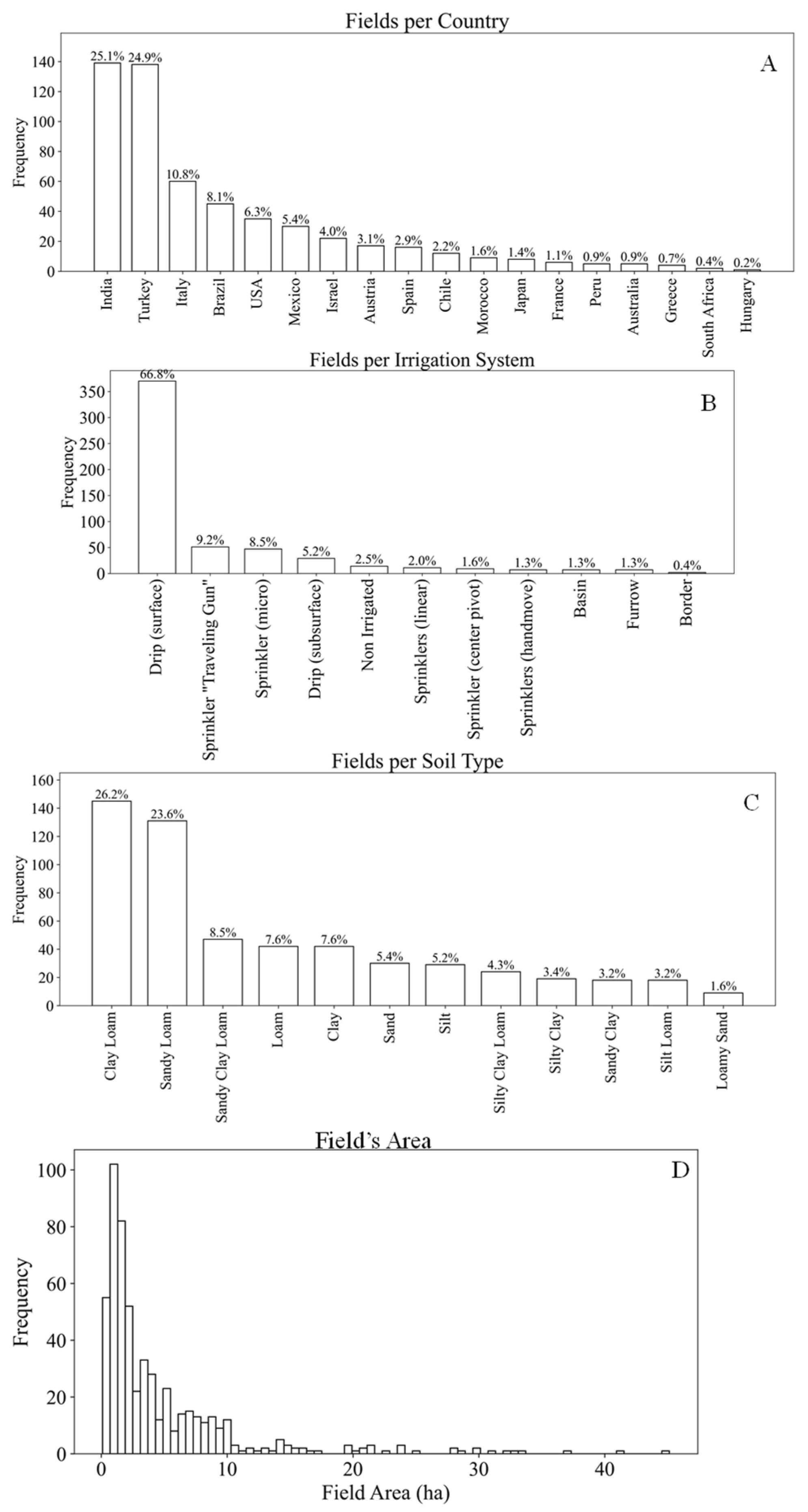
To test the SNAF, 548 commercial plots with 28 different crops from 18 countries were selected. Figure 1 and Table 1 illustrate the assortment of the fields used here, providing the distribution of the countries, field areas, soil types, irrigation systems, and crop types. The (not publicly available) source of these fields is the Manna Irrigation platform (Israel, Gvat, https://manna-irrigation.com, accessed on 25 March 2022), which is the developer of a sensor-free, software-only irrigation solution that delivers plot-specific irrigation recommendations. The soil type was determined according to the U.S. Department of Agriculture Textural Classification triangle method (see, for example, https://www.nrcs.usda.gov/wps/portal/nrcs/detail/soils/survey/?cid=nrcs142p2_054167, accessed on 26 August 2021).
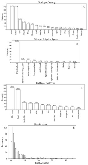
Figure 1.
Countries (A), irrigation systems (B), soil types (C), and field areas (D) in the distribution of the fields used in this study.

Table 1.
The crops used in this study.
2.2. NDVI Dataset
To obtain an NDVI time series per field, Google Earth Engine (GEE) [38] Python API was used. Using this tool, two-year (2020 and 2021) time series remote sensing imagery sets from Sentinel-2 level-2A (ground sampling distance—GSD 10 m) and Landsat-8 level-2 (GSD 30 m) were obtained for each field. These remote sensing imagery sets are already processed to the bottom of the atmosphere reflectance. Images with clouds, haze, cirrus, cloud shadows, snow, or ice, according to the relevant QA bands (SCL for Sentinel-2, and pixel_qa for Landsat-8), were removed from further analysis. Then, the NDVI was calculated, and all NDVI values (i.e., per-pixel NDVI) were averaged, for each image of the 548 fields, using:
where NIR and RED are the surface reflectance near-infrared and red spectral bands of Sentinel-2 (bands 8 and 4, respectively) and Landsat-8 (bands 5 and 4, respectively). The harmonization process between the Sentinel-2 and Landsat-8 NDVIs will be explained in Section 2.4.
2.3. SAR Dataset
The SAR (i.e., Sentinel-1) dataset was also obtained using GEE. The images used were all in the form of Interferometric Wide Swath Mode (IW) with dual polarization (VV + VH) and were acquired under level-1 processing as ground range detected (GRD). This IW mode is the main acquisition mode over land. Level-1 GRD products consist of focused SAR data projected to ground range using the Earth ellipsoid model WGS84 and have a GSD of 10 m. GEE preprocessed each scene with the Sentinel-1 Toolbox (https://sentinel.esa.int/web/sentinel/toolboxes/sentinel-1, accessed on 15 February 2022) using the following steps:
- Thermal noise removal
- Radiometric calibration
- Terrain correction using SRTM 30 or ASTER DEM for areas of a latitude greater than 60 degrees, where the SRTM is not available.
- The final terrain-corrected values are converted to decibels via log scaling (10*log10(x)).
2.4. Selecting SAR Indices for the SNAF
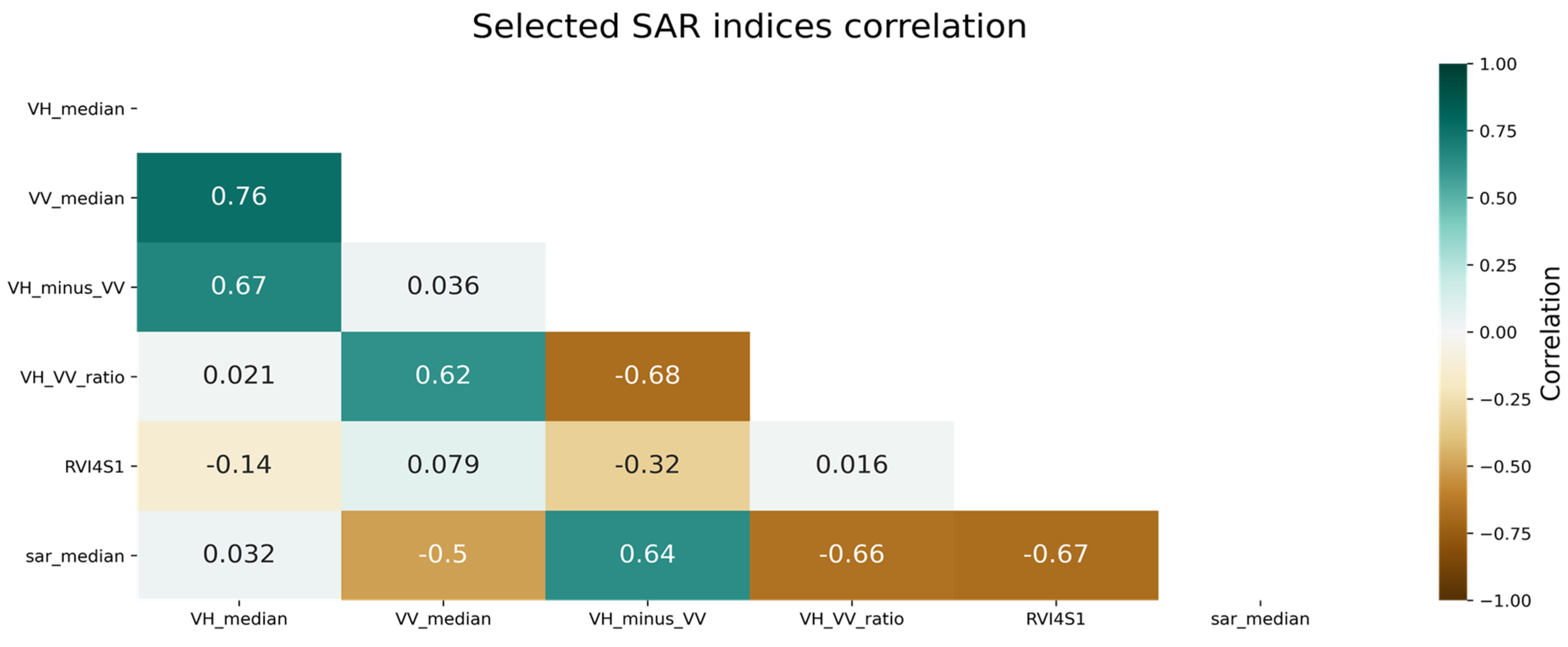
As mentioned, the SNAF utilizes several SAR indices, through a process that will be explained in the next section, to estimate the average NDVI of a field when the optical NDVI is not available. To choose which SAR indices will be used in the SNAF, seventeen Sentinel-1 indices were initially selected (Table 2). The correlation between the indices was calculated (Figure 2) based on 169,192 values of each index. According to Figure 2, some indices are highly correlated with others, suggesting redundancy. Based on this analysis, six indices with low collinearity were selected to be utilized in the SNAF method (Figure 3).
Table 2.
The SAR indices that were used in this study as the input for the random forest model. The source might contain a formula used to inspire the formula mentioned here. Note that some indices were not developed to estimate the NDVI directly; rather they are related to other crop parameters and hence may contribute to the SNAF method.
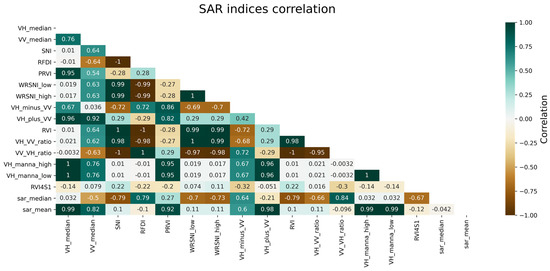
Figure 2.
Correlation between all (initial) seventeen SAR indices. Some of them are highly correlated with others. The correlation was calculated based on the 169,192 values each index had.
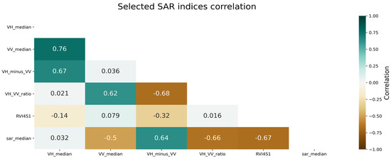
Figure 3.
Correlation between the six SAR indices with low correlation between them.
2.5. Estimating the NDVI from SAR Using the SNAF Method
The following steps describe the SNAF method and were executed for each date with a SAR image for each field. The process begins when a SAR image (SARlast_date) is available and an NDVI is not.
- The most recent NDVI date (NDVIlast_date) is obtained.
- The SNAF searches for all available NDVI and SAR data 365 days prior to the NDVIlast_date. Only these data are considered for further analysis.
- The SNAF generates a time series of the average NDVI value of the field from Sentinel-2 (NDVISN2) and Landsat-8 (NDVILS8).
- To harmonize between NDVISN2 and NDVILS8, their corresponding NDVI values are smoothed using a locally weighted regression (LWR) algorithm [42] (Figure 4). The LWR approximates the regression parameters for each point separately by iterating over them using the entire set of points, where a weight is assigned to each point as a function of its distance from the current point. LWR starts by defining a weight function:
Consequently, a sensor agnostic seamless NDVI time series is achieved (NDVIharmonized). This NDVIharmonized is later used as a reference for the model accuracy metric calculations.
- 5.
- After the LWR, a daily interpolation is applied to the NDVIharmonized (Figure 4) with the assumption that changes in crop growth are gradual during short periods [43]. This was done in order to achieve daily NDVI values, thus increasing the volume of the data for the machine learning model.
- 6.
- Five SAR time series indices (SAR5TS) (Figure 3, excluding sar_median) are calculated using the VV and VH bands of Sentinel-1. They are based on the SAR images from the last 365 days prior to the NDVIlast_date.
- 7.
- Steps #4 and #5 are applied to each of the SAR5TS. By doing that, a higher alignment between the SAR and the NDVI time series in terms of the number of values is reached, which enables more data for the model training (step #9).
- 8.
- The median of the five SAR indices (from step #6) is calculated, resulting in a total of six SAR time series indices (SAR6TS)
- 9.
- The random forest (RF) model [44] (with default settings) from the Python Scikit-Learn package [45] was utilized for the model training. The RF is a supervised learning algorithm that fits a number of decision trees on various sub-samples of the dataset and uses averaging to improve the predictive accuracy and control over-fitting. The inputs for the RF model are the NDVIharmonized (dependent variable) and the SAR6TS (independent variables). The training process of the RF model essentially learns the relationship between the NDVIharmonized and SAR6TS.
- 10.
- Once the training process is over, the RF makes an NDVI estimation (NDVISAR training) on the training set, thus creating an NDVI time series based on the SAR training data.
- 11.
- The LWR is deployed on the NDVISAR training.
- 12.
- A new time series (NDVIavg) is calculated by averaging the NDVIharmonized() and NDVISAR training.
- 13.
- To estimate the NDVI from the SARlast_date (i.e., when the SAR image exists and the NDVI does not), steps #6 and #8 are deployed on the SARlast_date image, thus creating six SAR values for the SARlast_date (SARlast_date6).
- 14.
- The SARlast_date6 is inserted into the trained RF model (step #9), resulting in an NDVI estimation (NDVISNAF_raw) from SAR.
- 15.
- The NDVISNAF_raw is added to the NDVIavg time series (step #12), and this entire time series is smoothed using the LWR. This step fine-tunes the NDVISNAF_raw value by compelling it to align with the previous data. This fine-tuned NDVISNAF_raw is the final output of the SNAF method and is hence termed NDVISNAF.
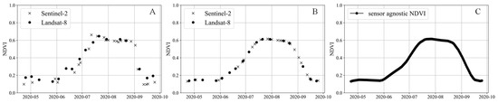
Figure 4.
A schematic illustration of steps #4 and #5. (A) shows the average NDVI from Sentinel-2 and Landsat-8 for a given field, with 43 data points; (B) displays the data points (n = 43) after LWR; and (C) depicts the results after the interpolation (linear line between the adjacent points) and the increase in data points (n = 156).

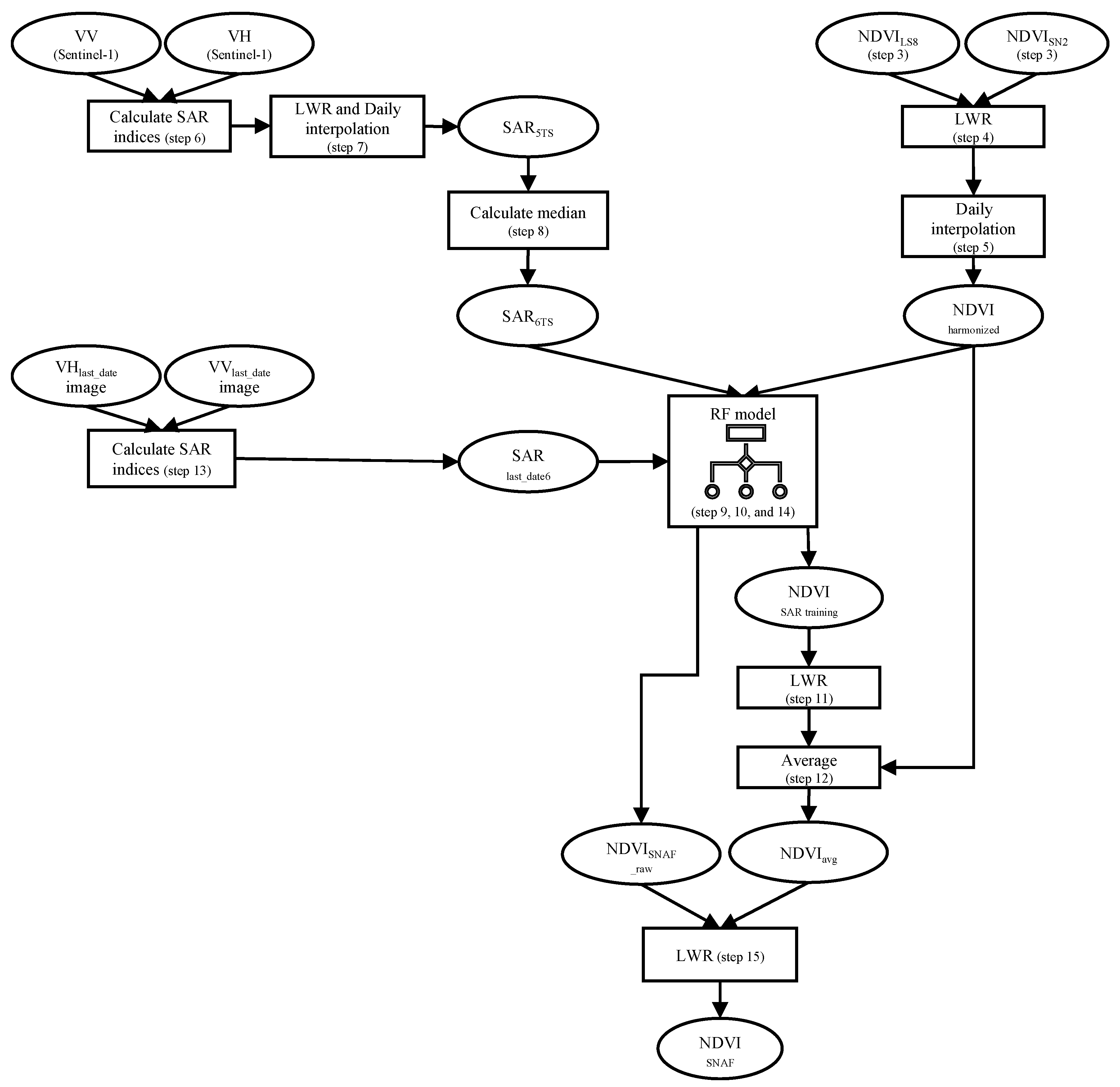
Figure 5 summarizes these steps in a flowchart. As mentioned, these steps were executed for each of the 548 fields for each available SAR image through 2021, thus creating real-world real-time scenarios when a SAR image is available but an optical NDVI image (i.e., one calculated from Sentinel-2 and Landsat-8) is not. It is important to mention that an agricultural growing season is less than one year long, meaning that the NDVI estimations by the SNAF were also applied for dates before and after the growing season months of 2021.
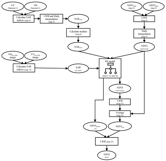
Figure 5.
Flowchart of the SNAF method, with the number of the corresponding steps in parentheses.
During the SNAF testing (i.e., while executing steps #1–15), some dates had both an SAR and NDVI. In these cases, the NDVI of that date was ignored in analysis, and the preceding NDVI date was considered as the NDVIlast_date (Step #1). This was done because the goal of this method is not to replace NDVI but rather to provide a solution when the NDVI is not available. In other words, when a clear optical image is available (i.e., an NDVI is available), there is no need for any SAR data or model. Moreover, from a statistical point of view, estimating the NDVI from SAR on a date when both are available will give optimistic results that will not reflect the robustness of the method.
In addition, the RF variable (i.e., SAR indices) importance (also termed the feature importance) for every SNAF scenario was recorded. This was done by utilizing the Scikit-Learn Permutation feature importance model (with its default settings). This model measures the importance of each variable (i.e., SAR index) by calculating the increase in the model’s prediction error after the variable values are randomly permuted. A variable is important if permuting its values increases the model error, because, in this case, the model relied on the feature for the prediction, and vice versa.
2.6. Accuracy Metrics
The accuracy metrics were calculated considering only the dates with both the optical NDVI and SAR, resulting in 6880 pairs of images. The measured NDVI (the ground truth for that matter) was the harmonized NDVI of the entire dataset (per field), and the estimated NDVI was the NDVISNAF. This harmonized NDVI of the entire dataset should not be confused with the NDVIharmoznied (mentioned in the steps in the previous section), which was part of the model training and was harmonized only on part of the data, i.e., 365 days from the NDVIlast_date for each iteration.
During the SNAF testing procedure, the optical NDVI values were ignored on the dates with both an SAR and optical NDVI. In other words, these optical NDVI values were not part of any model training and did not affect the SNAF method’s estimation of the NDVI.
Three accuracy metrics were chosen for the evaluation of the SNAF performance, namely, the bias, the root-mean-squared-error (RMSE), and the coefficient of determination (R2).
where Si and Mi are the estimated (NDVISNAF) and the measured (harmonized NDVI of the entire dataset, per field) value of the ith observation, respectively, is the average of M, and n is the number of observations.
The accuracy metrics considered only the dates with both an NDVI and SAR (no interpolated observations were included); however, most SAR images did not have a matching NDVI date and thus are not expressed in these metrics. Because it is important to observe how the NDVISNAF (as a time series) aligns with the harmonized NDVI of the entire dataset, per field (for all dates), a visual inspection was conducted by plotting both time series and observing the agreement.
3. Results
3.1. SNAF Performance for All Fields
A total of 6880 dates had both SAR and NDVI images. Figure 6 shows the NDVISNAF vs. NDVIharmonized results for all fields. The overall performance of the SNAF method is high, with an RMSE of 0.06, an R2 of 0.92, and a bias of 0.0, and the linear line between the NDVISNAF and NDVIharmonized is very close to the 1:1 line (the grey diagonal line in Figure 6), as expressed by the slope and intercept values.
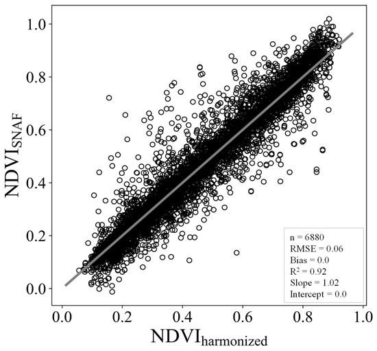
Figure 6.
Results for all fields and all dates. The grey line is the 1:1 line. Each dot represents the field’s average value.
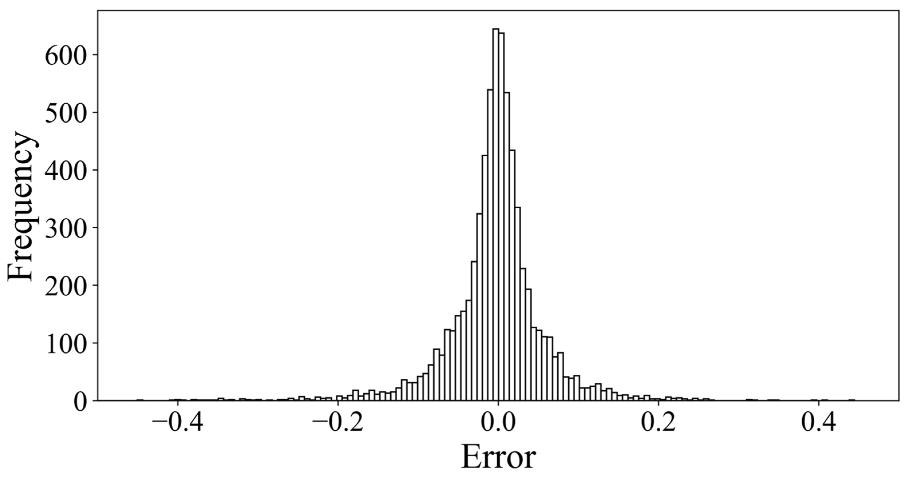
Figure 7 illustrates the distribution of all errors (NDVIharmonized-NDVISNAF). The errors are normally distributed around zero, which means the SNAF method is not biased in either direction and does not tend to overestimate or underestimate the NDVI.
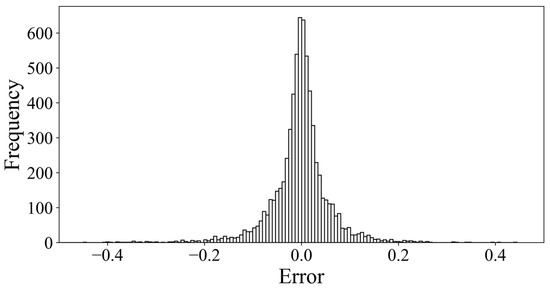
Figure 7.
The distribution of the NDVI errors (NDVIharmonized − NDVISNAF).
Table 3 presents how many fields had an absolute error greater than 0.1 and how many times this was the case. Most of the fields (76%) never had an absolute error > 0.1 or only had one once, while only 8.6% had this error four or more times.
Table 3.
Occurrences of an absolute error > 0.1 for all fields.
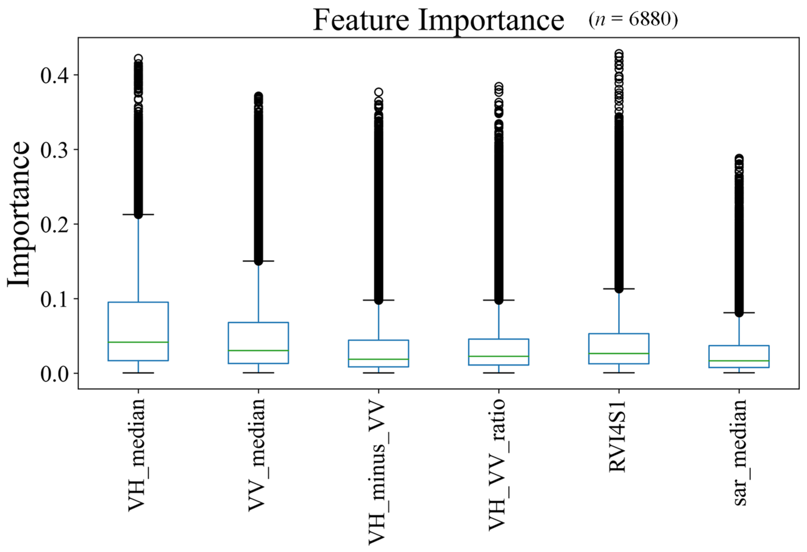
Figure 8 exhibits the importance of each SAR index in a boxplot. For each SAR date (for each field), the SNAF estimated the NDVI, and each SAR index had an importance value ranging between 0 and 1 for that estimation. The closer the value was to 1, the more important this index was for that specific NDVI estimation. For each NDVI estimation, the importance sum of all the indices was equal to 1. It can be seen that each of the 17 indices was important in a specific field at a specific point in time (Table 4 shows an example), meaning they were all useful. Generally, the VV_median, PRVI, VH_minus_VV, and RVI4S1 were more important than the others.
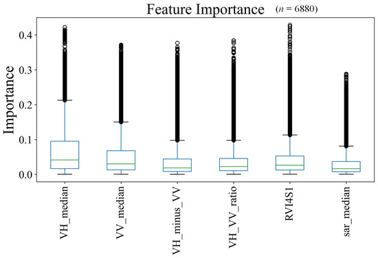
Figure 8.
Feature importance of all indices used in the SNAF method. The closer the importance is to 1, the more important that index was for a specific field for a specific point of time. Note that each index was important at some point in time.
Table 4.
Examples of different indices having the highest importance score (bold with underline) for different dates and fields.
3.2. SNAF Performance per Crop
Table 5 summarizes the SNAF performance per crop. The RMSE ranges from 0.02 to 0.1, which is considered a low and reasonable NDVI error. The bias for all crops is 0.0, and most of the crops have an R2 higher than 0.9. As expected, the crops with the lowest errors are orchards, either evergreen or deciduous. This is because the NDVI for these crops does not change dramatically during the year, as opposed to that for field crops. The crop with the highest errors is alfalfa, as expected, as it is a short-cycle crop. Because of its short cycles (~28 days per cycle), the NDVIs from Sentinel-2 and Landsat-8 are probably not frequent enough to capture the rapid changes in the NDVI, thus hampering the accuracy.
Table 5.
SNAF performance per crop (sorted by RMSE).
3.3. SNAF Performance as a Time Series
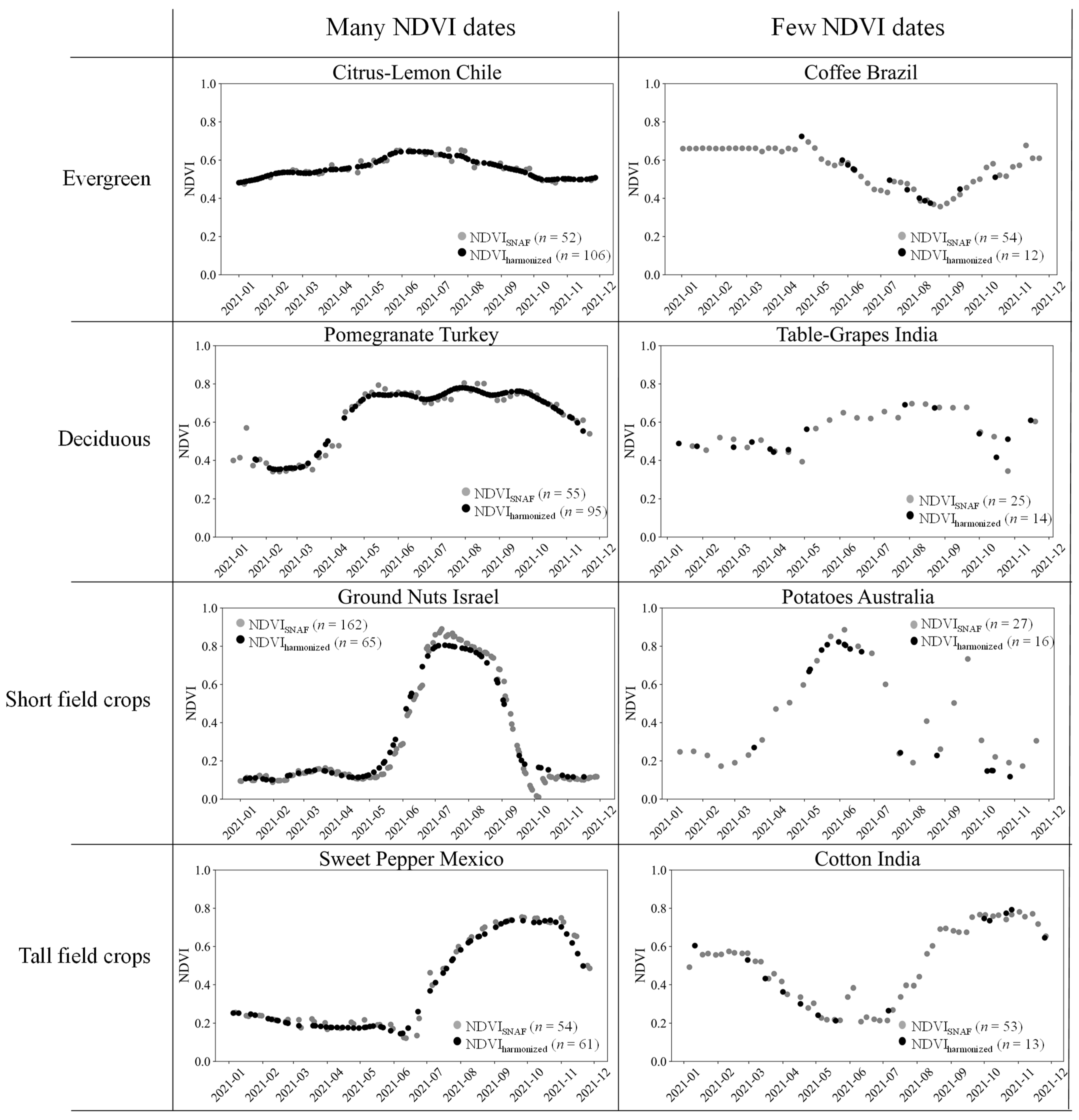
The results so far focused on comparing the NDVISNAF on the same date with the available NDVIharmonized, which demonstrated the robustness of the SNAF method. However, during this study, the SNAF method produced many more NDVISNAF values (~35,000) that have not been included in the evaluation so far simply because there was not a matching NDVIharmonized date. These other NDVISNAF values are important to visualize how the NDVISNAF aligns with the NDVIharmonized to create a seamless NDVI time series for the fields. To that end, eight fields representing cases of many or few NDVI values per crop group are presented in Figure 9.

Figure 9.
Eight examples visualizing the SNAF performance to estimate the NDVI across an entire year.
Figure 9 is a result of multiple SNAF runs (a run per SAR date). Each point in Figure 9 was generated based only on the past NDVI and SAR times series and did not consider any future data that are not available in real time.
The NDVISNAF shows a good agreement with the NDVI from optical sensors (NDVIharmonized), leading to a seamless NDVI time series. The SNAF was able to generate accurate SAR-estimated NDVI values even for fields with a relatively low number of optically based NDVI values. For example, the SNAF was able to capture the development phase of the cotton in India (15 July 2021 to 15 September 2021) and the potatoes in Australia (the end of March to May 2021) when the NDVI was not available for a long period (>1 month).
4. Discussion
The need to have a frequent and consistent provision of NDVI values increases with time as more and more companies, institutions, and end-users utilize Earth Observation (EO) datasets for their applications, research, workflows, and decision making. Commercial imaging companies such as Planet Labs (San Francisco, CA, United States) alleviate this need by generating massive and frequent EO image datasets. Nevertheless, some regions are susceptible to clouds, which is the main factor hampering the frequent and consistent provision of NDVI values. Moreover, regions that are not usually cloudy can still have short periods with a high cloud cover at crucial times—for example, when field crops emerge. To ensure frequent NDVI values for these cases, having more frequent optical images will not help, but utilizing SAR, which penetrates through clouds, will.
A method to estimate the NDVI from SAR should work globally (as does the NDVI), regardless of the field’s local conditions (e.g., crop and soil type). Achieving this is a great challenge because the SAR and the NDVI are sensitive to different vegetation properties. Consequently, the context (i.e., the local conditions) is an important factor that needs to be addressed when trying to overcome this challenge.
There are three approaches to addressing local conditions in this context. The first approach is to completely ignore the local conditions and assume similarity across all fields. This is essentially the case when using an index based on SAR polarimetric channels or a model with fixed coefficients, thus leading to unsatisfying NDVI results when applying it to different fields, reflecting limited applicability. The second is to obtain the local field conditions and possible auxiliary data, as suggested by [32], and incorporate them into the model. However, incorporating the local conditions will increase the model’s complexity and reduce its applicability, mainly because it is not possible to obtain the local field conditions for every field at every location, and these data are not always accurate or reliable. The third approach, which was adopted in this study, is to develop field- and time-specific models, thus making the task of incorporating the local conditions (e.g., soil and irrigation types, field topography, etc.) redundant because they hardly ever change with respect to one specific field.
It is true that, for field crops, crop rotation is a relatively common practice, and this was probably the case in some of the fields used here. The exact information regarding which crop was cultivated in 2020 was not available. Consequently, for some fields, the SNAF was trained on the NDVI–SAR data for the crop that was cultivated in 2020 and made the NDVI estimation on a different crop in 2021. Nevertheless, the SNAF accuracy indicates that the crop identity is less relevant.
The SNAF method suggested in this study generates multiple field- and time-specific models by training a new machine-learning model on the fly, per field, whenever a new SAR image is available. The outcome is a new estimated NDVI for a specific field for a specific time. Once a model generates this value, the model is disposable, meaning it will not be used again for NDVI estimations. In other words, once a new SAR image is available, the SNAF trains a new model and generates a new NDVI estimation. By doing that, the SNAF keeps the process simple and up to date and holds the local field conditions constant, eliminating the need to incorporate them into the model and enabling its global applicability, as it is not limited to a specific crop or to local conditions.
The SNAF method was tested on 548 commercial fields in 18 countries with 28 different crops through 2021, and the high performance is outlined in this study. The machine learning model used by the SNAF is the random forest, which was also found to be more useful than other models used in previous studies [29,36,46,47].
The overall RMSE of the SNAF method, based on 6880 paired SAR–NDVI images, was 0.06, which is better than the 0.08–0.11 value achieved by [36] (for rice, cotton, turmeric, and banana in India) and the 0.07 value achieved by [29] (for soybean and maize in Brazil), which did not use a large dataset for testing. Specifically, Ref. [36] reached an RMSE of 0.09 and an R2 of 0.76 for cotton, whereas the SNAF method, for cotton, had an RMSE of 0.05 and an R2 of 0.95 (Table 5). Ref. [37] used a self-developed SAR index and reported an R2 of 0.73 (different land uses in India) between the model estimation and the NDVI.
The potential of using SAR data to estimate the NDVI, as reported in previous studies, was manifested and validated by the SNAF method. The high accuracy metrics across the assortments of crops and countries show the method’s robustness in generating high-quality NDVI values globally.
Notwithstanding, SAR information cannot fully replace optical sensors in retrieving the NDVI; rather, it can only complement existing optical sensors. This is also specifically true for the SNAF method, as it depends on past NDVI time series for on-the-fly model training.
The SNAF method demonstrated here used the NDVI from two sources, namely, Sentinel-2 and Landsat-8, but more NDVI sources can be incorporated, which will probably lead to a higher accuracy. The source for the SAR data was the Sentinel-1 mission, which comprises a constellation of two polar-orbiting satellites (Sentinel-1A and Sentinel-1B) performing C-band imaging with VV and VH spectral bands. Incorporating other SAR sources is more complicated than incorporating optical sources, since they will have to have similar bands and similar preprocessing steps.
The SNAF was tested on dates in 2021 when Sentinel-1A and Sentinel-1B were both functioning as normal. However, since 23 December 2021, no data are being generated by Sentinel-1B due to power unit malfunction. The assumption is that this problem will continue for several months [48]. This means that Sentinel-1 data will be decreased by half for most of 2022. The implication for the SNAF is that less SAR data will be available in 2022 for model training. This decrease in data availability will not increase the SNAF accuracy, but it might not cause a decrease either (or at least a major decrease). Perhaps the available data for 2022 will be sufficient to generate good field- and time-specific models. Further investigation into this needs to be performed in the future.
Nevertheless, Sentinel-1 should not be considered as having permanently low availability, as ESA is considering moving up the already-planned Sentinel-1C and Sentinel-1D satellite launch, which will potentially triple the data availability and thus likely increase the SNAF accuracy.
The limitation of the SNAF method (and any other method based on SAR data) is that the SAR backscatter can differ and create artifacts when sudden (in terms of days) geometric or dielectric changes—as well as changes in the number of scatterers—are introduced. This might happen due to rain events or strong winds that can bend the crops (i.e., change the crop geometry), the rapid growth of weeds, litter due to pruning or trimming, or perhaps even irrigation events. In such cases, the SAR backscatter can be misleading, resulting in inaccurate NDVI estimations.
Future work should try to identify cases of strong wind or rain events via SAR backscatter and remove these values from the analysis. Further, more crop types should be tested with the SNAF method—predominantly rice, as it is a major grain crop that is usually irrigated by flood irrigation and can be challenging for an SAR-based method. In addition, more NDVI and perhaps even more SAR sources ought to be incorporated to account for cases where the current sources are not able to produce quality data.
5. Conclusions
This study introduced the SNAF (Sentinel-1 to NDVI for Agricultural Fields) method. The goal of the SNAF method is to estimate the NDVI from Sentinel-1 data for any field and crop anywhere and anytime. To do that, the SNAF calculates six SAR time series indices and uses them as independent variables in the random forest model, where the dependent variable is the NDVI time series. The SNAF is deployed every time a new SAR image is available because the relationship between SAR and the NDVI is not consistent, thus enabling a field- and time-specific NDVI estimation, which is flexible and up to date. The SNAF is based solely on the SAR and NDVI time series per field and per point in time, therefore reducing the complexity and eliminating the need to incorporate additional auxiliary and local field data that are not always obtainable or accurate.
The SNAF method was tested on a large dataset—something that is not found in previous studies—comprised of 548 commercial fields with 28 crops across 18 countries throughout 2021. The results show the model’s high performance, with RMSE, bias, and R2 values of 0.06, 0.00, and 0.92 respectively, expressing the model’s robustness and global applicability.
Author Contributions
Conceptualization, R.P. and O.B.; Data curation, R.P.; Formal analysis, R.P.; Investigation, O.B.; Methodology, R.P. and O.B.; Project administration, T.S.; Supervision, O.B. and T.S.; Visualization, R.P. and R.T.; Writing—original draft, R.P.; Writing—review & editing, R.P., O.B., R.T. and T.S. All authors have read and agreed to the published version of the manuscript.
Funding
This research received no external funding.
Data Availability Statement
Not applicable.
Conflicts of Interest
The authors declare no conflict of interest.
References
- Rouse, J.W., Jr.; Haas, R.H.; Schell, J.A.; Deering, D.W. Monitoring Vegetation Systems in the Great Plains with Erts. NASA Spec. Publ. 1974, 351, 309. [Google Scholar]
- Tucker, C.J. Red and Photographic Infrared Linear Combinations for Monitoring Vegetation. Remote Sens. Environ. 1979, 8, 127–150. [Google Scholar] [CrossRef] [Green Version]
- Veloso, A.; Mermoz, S.; Bouvet, A.; Le Toan, T.; Planells, M.; Dejoux, J.-F.; Ceschia, E. Understanding the Temporal Behavior of Crops Using Sentinel-1 and Sentinel-2-like Data for Agricultural Applications. Remote Sens. Environ. 2017, 199, 415–426. [Google Scholar] [CrossRef]
- USGS NDVI, the Foundation for Remote Sensing Phenology|U.S. Geological Survey. Available online: https://www.usgs.gov/special-topics/remote-sensing-phenology/science/ndvi-foundation-remote-sensing-phenology?qt-science_center_objects=0#qt-science_center_objects (accessed on 11 February 2022).
- Purkis, S.J.; Klemas, V.V. Remote Sensing and Global Environmental Change, 1st ed.; Wiley-Blackwell: Chichester, UK; Hoboken, NJ, USA, 2011; ISBN 978-1-4051-8225-6. [Google Scholar]
- Defries, R.S.; Townshend, J.R.G. NDVI-Derived Land Cover Classifications at a Global Scale. Int. J. Remote Sens. 1994, 15, 3567–3586. [Google Scholar] [CrossRef]
- Fuller, D.O. Trends in NDVI Time Series and Their Relation to Rangeland and Crop Production in Senegal, 1987–1993. Int. J. Remote Sens. 1998, 19, 2013–2018. [Google Scholar] [CrossRef]
- Huang, J.; Wang, H.; Dai, Q.; Han, D. Analysis of NDVI Data for Crop Identification and Yield Estimation. IEEE J. Sel. Top. Appl. Earth Obs. Remote Sens. 2014, 7, 4374–4384. [Google Scholar] [CrossRef]
- Bausch, W.; Neale, C. Crop Coefficients Derived from Reflected Canopy Radiation: A Concept. Trans. ASAE 1987, 30, 703–709. [Google Scholar] [CrossRef]
- Beeri, O.; Pelta, R.; Shilo, T.; Mey-tal, S.; Tanny, J. Accuracy of Crop Coefficient Estimation Methods Based on Satellite Imagery. In Precision Agriculture’19; Wageningen Academic Publishers: Wageningen, The Netherlands, 2019; p. 444. [Google Scholar]
- Tasumi, M.; Allen, R.; Trezza, R. Calibrating Satellite-Based Vegetation Indices to Estimate Evapotranspiration and Crop Coefficients. In Proceedings of the 2006 USCID Water Management Conference, Ground Water and Surface Water under Stress: Competition, Interaction, Solutions, Denver, Boise, ID, USA, 25–28 October 2006; pp. 103–112. [Google Scholar]
- Colombo, R.; Bellingeri, D.; Fasolini, D.; Marino, C.M. Retrieval of Leaf Area Index in Different Vegetation Types Using High Resolution Satellite Data. Remote Sens. Environ. 2003, 86, 120–131. [Google Scholar] [CrossRef]
- Fan, L.; Gao, Y.; Brück, H.; Bernhofer, C. Investigating the Relationship between NDVI and LAI in Semi-Arid Grassland in Inner Mongolia Using in-Situ Measurements. Appl Clim. 2009, 95, 151–156. [Google Scholar] [CrossRef]
- van Wijk, M.T.; Williams, M. Optical Instruments for Measuring Leaf Area Index in Low Vegetation: Application in Arctic Ecosystems. Ecol. Appl. 2005, 15, 1462–1470. [Google Scholar] [CrossRef] [Green Version]
- Calera, A.; Martínez, C.; Melia, J. A Procedure for Obtaining Green Plant Cover: Relation to NDVI in a Case Study for Barley. Int. J. Remote Sens. 2001, 22, 3357–3362. [Google Scholar] [CrossRef]
- Carlson, T.N.; Ripley, D.A. On the Relation between NDVI, Fractional Vegetation Cover, and Leaf Area Index. Remote Sens. Environ. 1997, 62, 241–252. [Google Scholar] [CrossRef]
- Tenreiro, T.R.; García-Vila, M.; Gómez, J.A.; Jiménez-Berni, J.A.; Fereres, E. Using NDVI for the Assessment of Canopy Cover in Agricultural Crops within Modelling Research. Comput. Electron. Agric. 2021, 182, 106038. [Google Scholar] [CrossRef]
- Arnall, D.B.; Abit, M.J.M.; Taylor, R.K.; Raun, W.R. Development of an NDVI-Based Nitrogen Rate Calculator for Cotton. Crop Sci. 2016, 56, 3263–3271. [Google Scholar] [CrossRef]
- Jewiss, J.L.; Brown, M.E.; Escobar, V.M. Satellite Remote Sensing Data for Decision Support in Emerging Agricultural Economies: How Satellite Data Can Transform Agricultural Decision Making [Perspectives]. IEEE Geosci. Remote Sens. Mag. 2020, 8, 117–133. [Google Scholar] [CrossRef]
- Johnson, L.F.; Trout, T.J. Satellite NDVI Assisted Monitoring of Vegetable Crop Evapotranspiration in California’s San Joaquin Valley. Remote Sens. 2012, 4, 439–455. [Google Scholar] [CrossRef] [Green Version]
- Lukina, E.V.; Freeman, K.W.; Wynn, K.J.; Thomason, W.E.; Mullen, R.W.; Stone, M.L.; Solie, J.B.; Klatt, A.R.; Johnson, G.V.; Elliott, R.L.; et al. Nitrogen Fertilization Optimization Algorithm Based on In-Season Estimates of Yield and Plant Nitrogen Uptake. J. Plant Nutr. 2001, 24, 885–898. [Google Scholar] [CrossRef]
- Moran, M.S.; Inoue, Y.; Barnes, E.M. Opportunities and Limitations for Image-Based Remote Sensing in Precision Crop Management. Remote Sens. Environ. 1997, 61, 319–346. [Google Scholar] [CrossRef]
- Toureiro, C.; Serralheiro, R.; Shahidian, S.; Sousa, A. Irrigation Management with Remote Sensing: Evaluating Irrigation Requirement for Maize under Mediterranean Climate Condition. Agric. Water Manag. 2017, 184, 211–220. [Google Scholar] [CrossRef]
- Wall, L.; Larocque, D.; Léger, P. The Early Explanatory Power of NDVI in Crop Yield Modelling. Int. J. Remote Sens. 2008, 29, 2211–2225. [Google Scholar] [CrossRef]
- King, M.D.; Platnick, S.; Menzel, W.P.; Ackerman, S.A.; Hubanks, P.A. Spatial and Temporal Distribution of Clouds Observed by MODIS Onboard the Terra and Aqua Satellites. IEEE Trans. Geosci. Remote Sens. 2013, 51, 3826–3852. [Google Scholar] [CrossRef]
- Richards, J.A. Remote Sensing with Imaging Radar; Springer: Heidelberg, Germany; New York, NY, USA, 2009; ISBN 978-3-642-02019-3. [Google Scholar]
- Reiche, J.; Verbesselt, J.; Hoekman, D.; Herold, M. Fusing Landsat and SAR Time Series to Detect Deforestation in the Tropics. Remote Sens. Environ. 2015, 156, 276–293. [Google Scholar] [CrossRef]
- Flores, A.; Herndon, K.; Thapa, R.; Cherrington, E. The SAR Handbook: Comprehensive Methodologies for Forest Monitoring and Biomass Estimation; NASA: Washington, DC, USA, 2019. [Google Scholar]
- Filgueiras, R.; Mantovani, E.C.; Althoff, D.; Fernandes Filho, E.I.; Cunha, F.F. da Crop NDVI Monitoring Based on Sentinel 1. Remote Sens. 2019, 11, 1441. [Google Scholar] [CrossRef] [Green Version]
- Moran, M.S.; Hymer, D.C.; Qi, J.; Kerr, Y. Comparison of ERS-2 SAR and Landsat TM Imagery for Monitoring Agricultural Crop and Soil Conditions. Remote Sens. Environ. 2002, 79, 243–252. [Google Scholar] [CrossRef]
- Frison, P.-L.; Fruneau, B.; Kmiha, S.; Soudani, K.; Dufrêne, E.; Le Toan, T.; Koleck, T.; Villard, L.; Mougin, E.; Rudant, J.-P. Potential of Sentinel-1 Data for Monitoring Temperate Mixed Forest Phenology. Remote Sens. 2018, 10, 2049. [Google Scholar] [CrossRef] [Green Version]
- Holtgrave, A.-K.; Röder, N.; Ackermann, A.; Erasmi, S.; Kleinschmit, B. Comparing Sentinel-1 and -2 Data and Indices for Agricultural Land Use Monitoring. Remote Sens. 2020, 12, 2919. [Google Scholar] [CrossRef]
- Kaushik, S.K.; Mishra, V.N.; Punia, M.; Diwate, P.; Sivasankar, T.; Soni, A.K. Crop Health Assessment Using Sentinel-1 SAR Time Series Data in a Part of Central India. Remote Sens Earth Syst Sci 2021, 4, 217–234. [Google Scholar] [CrossRef]
- Navarro, A.; Rolim, J.; Miguel, I.; Catalão, J.; Silva, J.; Painho, M.; Vekerdy, Z. Crop Monitoring Based on SPOT-5 Take-5 and Sentinel-1A Data for the Estimation of Crop Water Requirements. Remote Sens. 2016, 8, 525. [Google Scholar] [CrossRef] [Green Version]
- Mazza, A.; Gargiulo, M.; Scarpa, G.; Gaetano, R. Estimating the NDVI from SAR by Convolutional Neural Networks. In Proceedings of the IGARSS 2018—2018 IEEE International Geoscience and Remote Sensing Symposium, Valencia, Spain, 22–27 July 2018; pp. 1954–1957. [Google Scholar]
- Mohite, J.D.; Sawant, S.A.; Pandit, A.; Pappula, S. Investigating the Performance of Random Forest and Support Vector Regression for Estimation of Cloud-Free Ndvi Using SENTINEL-1 SAR Data. ISPRS-Int. Arch. Photogramm. Remote Sens. Spat. Inf. Sci. 2020, 43B3, 1379–1383. [Google Scholar] [CrossRef]
- Periasamy, S. Significance of Dual Polarimetric Synthetic Aperture Radar in Biomass Retrieval: An Attempt on Sentinel-1. Remote Sens. Environ. 2018, 217, 537–549. [Google Scholar] [CrossRef]
- Gorelick, N.; Hancher, M.; Dixon, M.; Ilyushchenko, S.; Thau, D.; Moore, R. Google Earth Engine: Planetary-Scale Geospatial Analysis for Everyone. Remote Sens. Environ. 2017, 202, 18–27. [Google Scholar] [CrossRef]
- Chang, J.G.; Shoshany, M.; Oh, Y. Polarimetric Radar Vegetation Index for Biomass Estimation in Desert Fringe Ecosystems. IEEE Trans. Geosci. Remote Sens. 2018, 56, 7102–7108. [Google Scholar] [CrossRef]
- Trudel, M.; Charbonneau, F.; Leconte, R. Using RADARSAT-2 Polarimetric and ENVISAT-ASAR Dual-Polarization Data for Estimating Soil Moisture over Agricultural Fields. Can. J. Remote Sens. 2012, 38, 514–527. [Google Scholar] [CrossRef]
- Gitelson, A.A. Wide Dynamic Range Vegetation Index for Remote Quantification of Biophysical Characteristics of Vegetation. J Plant Physiol 2004, 161, 165–173. [Google Scholar] [CrossRef] [PubMed] [Green Version]
- Atkeson, C.G.; Moore, A.W.; Schaal, S. Locally Weighted Learning. In Lazy Learning; Aha, D.W., Ed.; Springer: Dordrecht, The Netherlands, 1997; pp. 11–73. ISBN 978-94-017-2053-3. [Google Scholar]
- Fieuzal, R.; Baup, F.; Marais-Sicre, C. Monitoring Wheat and Rapeseed by Using Synchronous Optical and Radar Satellite Data—From Temporal Signatures to Crop Parameters Estimation. Adv. Remote Sens. 2013, 2, 162–180. [Google Scholar] [CrossRef] [Green Version]
- Breiman, L. Random Forests. Mach. Learn. 2001, 45, 5–32. [Google Scholar] [CrossRef] [Green Version]
- Pedregosa, F.; Varoquaux, G.; Gramfort, A.; Michel, V.; Thirion, B.; Grisel, O.; Blondel, M.; Prettenhofer, P.; Weiss, R.; Dubourg, V.; et al. Scikit-Learn: Machine Learning in Python. J. Mach. Learn. Res. 2011, 12, 2825–2830. [Google Scholar]
- Kumar, P.; Prasad, R.; Gupta, D.K.; Mishra, V.N.; Vishwakarma, A.K.; Yadav, V.P.; Bala, R.; Choudhary, A.; Avtar, R. Estimation of Winter Wheat Crop Growth Parameters Using Time Series Sentinel-1A SAR Data. Geocarto Int. 2018, 33, 942–956. [Google Scholar] [CrossRef]
- Vreugdenhil, M.; Wagner, W.; Bauer-Marschallinger, B.; Pfeil, I.; Teubner, I.; Rüdiger, C.; Strauss, P. Sensitivity of Sentinel-1 Backscatter to Vegetation Dynamics: An Austrian Case Study. Remote Sens. 2018, 10, 1396. [Google Scholar] [CrossRef] [Green Version]
- Copernicus Sentinel-1B Anomaly (5th Update). Available online: https://sentinels.copernicus.eu/web/sentinel/-/copernicus-sentinel-1b-anomaly-5th-update/1.2?redirect=%2Fweb%2Fsentinel%2Fmissions%2Fsentinel-1 (accessed on 7 March 2022).


Publisher’s Note: MDPI stays neutral with regard to jurisdictional claims in published maps and institutional affiliations. |
© 2022 by the authors. Licensee MDPI, Basel, Switzerland. This article is an open access article distributed under the terms and conditions of the Creative Commons Attribution (CC BY) license (https://creativecommons.org/licenses/by/4.0/).