SlideSim: 3D Landslide Displacement Monitoring through a Physics-Based Simulation Approach to Self-Supervised Learning

Abstract

Displacement monitoring is a critical step to understand, manage, and mitigate potential landside hazard and risk. Remote sensing technology is increasingly used in landslide monitoring. While significant advances in data collection and processing have occurred, much of the analysis of remotely-sensed data applied to landslides is still relatively simplistic, particularly for landslides that are slow moving and have not yet “failed”. To this end, this work presents a novel approach, SlideSim, which trains an optical flow predictor for the purpose of mapping 3D landslide displacement using sequential DEM rasters. SlideSim is capable of automated, self-supervised learning by building a synthetic dataset of displacement landslide DEM rasters and accompanying label data in the form of u/v pixel offset flow grids. The effectiveness, applicability, and reliability of SlideSim for landslide displacement monitoring is demonstrated with real-world data collected at a landslide on the Southern Oregon Coast, U.S.A. Results are compared with a detailed ground truth dataset with an End Point Error RMSE = 0.026 m. The sensitivity of SlideSim to the input DEM cell size, representation (hillshade, slope map, etc.), and data sources (e.g., TLS vs. UAS SfM) are rigorously evaluated. SlideSim is also compared to diverse methodologies from the literature to highlight the gap that SlideSim fills amongst current state-of-the-art approaches.

1. Introduction

Reliable and accurate monitoring of landslides is critical to manage and mitigate potential hazards and risk to communities and their infrastructure. Continued advances in surveying and remote sensing technologies [1,2,3] have enabled frequent collection of high resolution, high accuracy data with the potential to measure landslide movement with superior spatial resolution compared to conventional methods such as inclinometers, extensometers and GNSS monitoring [4,5,6]. Nevertheless, in practice, remote sensing data analysis approaches tend to be either overly simplistic in nature or require intensive manual processing such as expert development of site-specific data processing and parameter derivation. Simultaneously, recent advances in the field of computer vision have demonstrated the suitability of deep learning approaches to RGB image- and video-based optical flow problems, which now achieve amongst the best performance on many widely used testing datasets [7,8,9,10]. Building on these advances, this paper develops and rigorously validates a deep learning approach for the task of landslide displacement mapping using geospatial DEMs (Digital Elevation Models) derived from remote sensing methods.

In situ landslide monitoring can include drilling boreholes to house inclinometers, piezometers and other instrumentation to characterize the driving mechanisms, modes, and extent of failure. These instruments produce displacement readings with depth, which can be used to further understand the landslide kinematics, assist with rendering informed decisions regarding landslide activity, provide estimates of damage, and identify potential mitigation strategies. Notwithstanding, subsurface exploration is time-consuming, potentially hazardous, and often cost-prohibitive, especially for stakeholders burdened with numerous landslides or large landslides. Due to these challenges, subsurface exploration and instrumentation often can only be conducted at several discrete locations within the landslide body and thus relies heavily on interpolation methods to infer landslide properties across its entire spatial extent. The installed instrumentation is also subject to shearing/damage under modest movements and thus does not serve as a permanent monitoring solution.

Remote sensing and surveying monitoring approaches are increasingly used in landslide monitoring and many other earth science applications. TLS (terrestrial laser scanning), for example, can produce high-resolution point clouds useful for monitoring slope deformation [11,12,13]. More recently, UAS lidar systems have become capable of mapping the surface of large landslides while maintaining satisfactory accuracy and coverage [14]. Photogrammetric data collected via UAS platforms can generate both high-resolution, orthorectified images, and point clouds using SfM (structure from motion) and MVS (multiview stereopsis) techniques [15]. Photogrammetric technology typically have a lower cost of entry compared to lidar and can provide a similar level of accuracy to UAS lidar methods for sparsely vegetated terrain if appropriate data collection and processing methods are followed [16].

Once data are collected using the approaches highlighted above, additional processing must be performed to be effective in application to landslide analysis and monitoring. Data must first be georeferenced using methods appropriate for the field methods and equipment used [17,18,19]. The next step is to identify the ground surface within the point cloud using a ground filter [20,21]. At this point a terrain model representing the landslide terrain can be constructed, typically in the form of a DEM (Digital Elevation Model). The detail of the DEM depends on the quality of the source input data and the desired model resolution. When needed, a variety of hole filling (i.e., interpolation) techniques help reduce data gaps within the model (e.g., [22]).

While important advances in both the data collection and processing of remotely sensed DEMs continue to occur, much of the analysis using these data in application to landslides can still be considered simplistic relative to the amount of information actually contained within the data. For example, creating an elevation change grid by differencing sequentially collected DEMs on a per pixel basis is one of the most widely used analysis techniques given that this grid can be used to estimate volumetric changes throughout a landslide [23]. However, while this type of analysis is useful in rockfall or seacliff monitoring, it may not be representative when applied to landslides undergoing compression, extension, or that are not fully evacuated.

Moving beyond the 1D elevation change analysis, three-dimensional (3D) displacement vectors can be generated from sequential datasets by tracking distinct points and/or features representing an object between two datasets. Feature tracking can be accomplished by using manual extraction methods, semi-automated feature extraction methods for distinct objects such as tree trunks [24], geomorphological features [25], or windowed registration/correspondence methods such as Iterative Closest Point (ICP) [26]. Nevertheless, these methods may be subjective and still require expert knowledge to select suitable tracking features. They also tend to be computationally expensive since they directly use the point cloud.

In contrast, image correlation approaches using sequential orthorectified imagery can generate 2D horizontal displacement vectors. Such approaches include PIV (particle image velocimetry) [27,28], Optical flow [29], COSI-Corr (Co-registration of Optically Sensed Images and Correlation) [30], Optical image correlation [31,32], and other image correlation methods [33]. Such methods are sensitive to variance in pixel illumination (lighting), and land cover change (such as vegetation growth or seasonal changes), which can result in erroneous displacement vectors when substantial time has elapsed between surveys [33]. Correlation approaches can also be applied to DEMs in addition to images. Unlike optical images, when proper data collection/preparation is used, DEMs can produce consistent maps that are more robust to seasonal changes and do not suffer from variance in pixel illumination. However, visual representations of DEMs, in their basic form of encoded elevation values, can often lack texture (e.g., smooth road and flat areas of grassland) and can contain areas of repeating patterns/edges (guard rails, pavement markings, fencing etc.). Hence, using the DEM for analysis proves difficult for the majority of correlation approaches that rely on gradient-based matching.

With recent advances in computer vision, these well-established image correlation techniques have been surpassed by learning-based approaches [9]. Deep learning approaches use synthetically generated video datasets, such as the MPI-Sintel dataset [34] or the FlyingChairs dataset [35] where a known optical flow grid (grid of u and v pixel displacement) is available for each neighboring frame pair such that it is suitable as training data. The first popularized model, Flownet [35], proposed two CNN-based architectures (Convolutional Neural Network). The first consists solely of convolutional layers where the two input images are stacked before being input into the model (FlownetSimple). The second model (FlowNetCorr) consists of a series of feature extraction convolutional layers where each image is processed individually, followed by a correlational layer which performs a comparison of the two feature maps, and then followed by additional convolutional layers. These models perform better than traditional methods on data similar to the training dataset; however, they do not perform as well on more generalized datasets [35]. Subsequently, Flownet2 built upon the original framework by modifying the order of training data and implementing a stacked architecture composed of specialized sub-networks [7]. Flownet2 performs similarly, and in some cases better than traditional methods; however, because Flownet2 is a very large network composed of many different sub-networks, the training process is more difficult. More recently, RAFT (Recurrent All-Pairs Field Transforms) [10] achieved state-of-the-art performance utilizing the same training data as Flownet, with a model composed of a feature extraction stage built from a series of residual layers followed by the creation of 4D correlation volumes which is then fed into a sequence of GRU cells (Gated Recurrent Unit) that iteratively updates the flow field. The resulting model has fewer parameters than Flownet2 while exceeding the performance of traditional methods on many of the benchmark datasets.

To overcome these limitations, this work presents a novel approach, SlideSim, which effectively trains an optical flow predictor to specifically map 3D landslide displacement using sequential DEM raster images. SlideSim can automate the generation of realistic synthetic data of displaced landslide DEM rasters along with their accompanying label data in the form of u/v (x/y-axis image coordinate velocities) pixel offset flow grids. SlideSim enables networks to be trained using a self-supervised framework, removing the barrier presented by the lack of available labelled field data for training. SlideSim offers many advantages over variational image correlation approaches: (1) it does not require manual tuning of feature extraction parameters, (2) additional synthetic data/training can be conducted before inference on a new site to learn any site-specific features, and (3) SlideSim can also output 3D displacement vectors compared with the 2D displacements available from image correlation. The applicability and reliability of SlideSim for use in landslide displacement mapping is demonstrated with real-world data collected at a landslide on the Southern Oregon Coast in the USA through comparison with a manually-generated ground truth dataset to evaluate the sensitivity of the network to the input DEM raster (cell size, raster representation) and assess how the input data source (TLS, UAS SfM) impacts the displacement mapping results.

2. Materials and Methods

SlideSim is a novel approach to enable self-supervised learning of 3D landslide displacement monitoring using sequential DEM rasters as input. SlideSim consists of three primary steps:

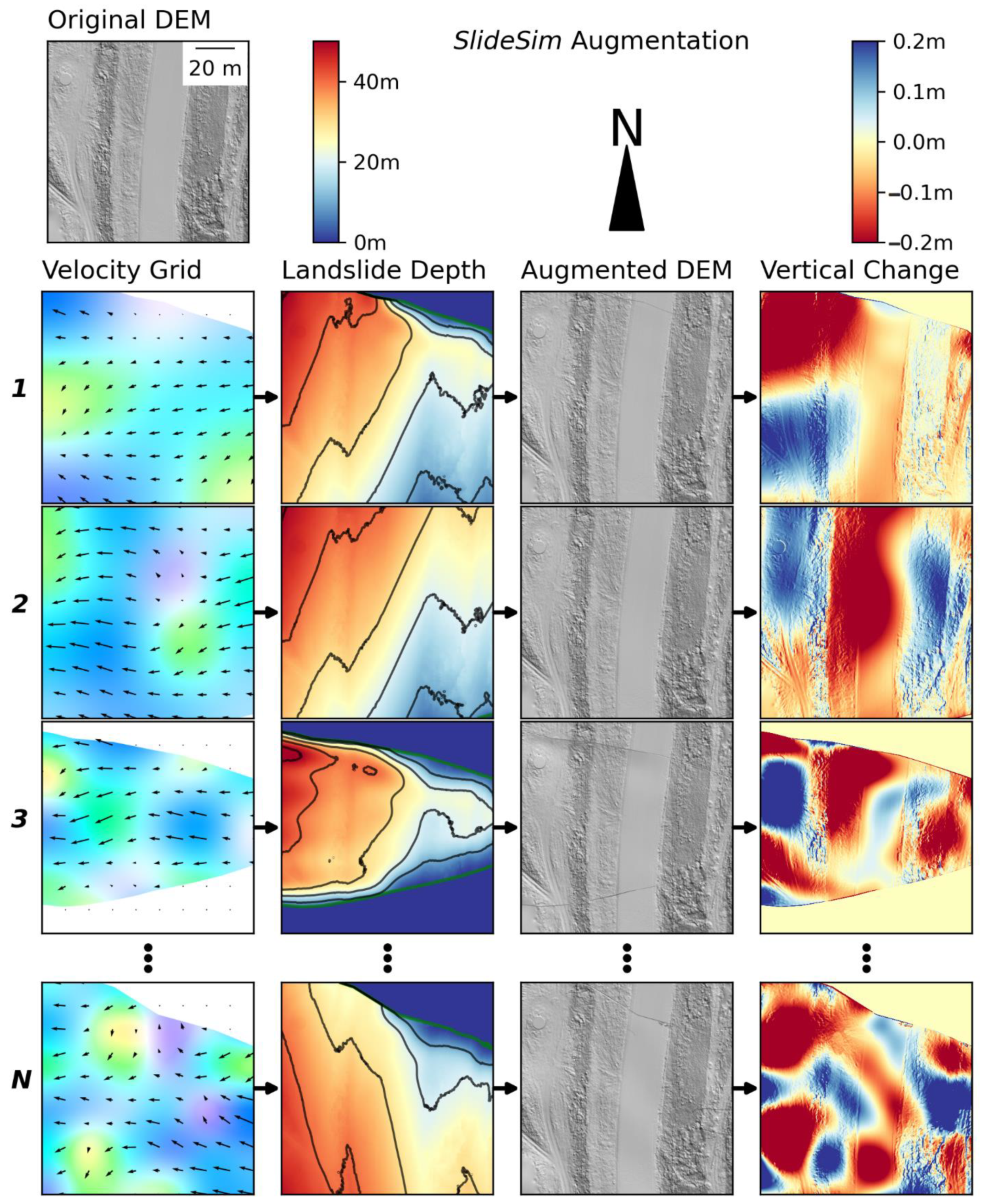
• Generation and simulation of synthetic training data through deterministic modeling of the landslide surface using a conservation of mass (COM) approach for many different input scenarios;
• End-to-end training of an optical flow predictor network using RAFT architecture and transfer learning followed by training on the simulated dataset;
• Inference and calculation of the 3D landslide displacement vector map by first feeding sequential DEM rasters through the trained model to generate 2D horizontal displacement vectors followed by deterministic computation of the vertical component of displacement.

2.1. Simulation and Generation of Synthetic Training Data

A synthetic dataset of labeled displaced landslide DEM rasters is generated to train the optical flow predictor using a self-supervised learning process, where the supervisory signal used in training is generated in an automated process. Synthetic data enable a sufficient amount of training data, which are impractical to collect and hand label from sets of pre- and post-movement DEMs of actual landslide movements. To generate the synthetic data, a physics-based, conservation of mass (COM) approach similar to that described in [36] is used. The principle of conservation of mass states that the mass of a closed system must remain constant over time. Using this principle and assuming incompressible behavior and rigid basal motion, the change in elevation across the landslide can be computed such that the mass of the landslide remains constant for a given set of boundary conditions (landslide boundary and slip surface) and a given velocity field. By using the finite difference method via the central difference method, if raster cells containing the landslide depth (m), and surface velocities (m/epoch) are known, or in this case assumed, the elevation of each cell in a DEM of a landslide can be updated for each epoch of movement:

$$-\frac{\partial z}{\partial t}=h_t\frac{\partial vel}{\partial L}+ve{l}_t\frac{\partial h}{\partial L}$$

(1)

where z is the ground surface elevation, t is the epoch, h is the landslide depth, vel is the landslide horizontal velocity, and L is the horizontal change. Equation (1) can be expanded for each horizontal velocity component:

$$-\frac{\partial z}{\partial t}=h_t\frac{\partial u}{\partial x}+u_t\frac{\partial h}{\partial x}+h_t\frac{\partial v}{\partial y}+v_t\frac{\partial h}{\partial y}$$

(2)

where u and v are the x/y components of velocity, respectively, and x and y are the positional components along the x/y-axis, respectively, such that ∂x and ∂y correspond with the cell size of the finite grid in the approach used. From Equation (2), the ground elevation, and the landslide depth can be iteratively updated through for N movement epochs (representing time) as shown in Equations (3) and (4):

$$Z_t=Z_{t-1}-\frac{\partial z}{\partial t}$$

(3)

$$h_t=Z_t-S$$

(4)

where S is the elevation of the landslide slip surface at each pixel. This approach allows a synthetic DEM raster representing the displaced landslide to be generated over N movement epochs using finite grids representing unique landslide boundary grids, landslide slip surface elevations (SSEM), and horizontal velocity rates. If realistic examples of the above finite grids are generated, then the number of unique synthetic DEM rasters representing example displaced landslides is the product of the number of each finite grid:

$$N_{syntheticDEMs}=N_{initialDEMs}\times N_{bounds}\times N_{SSEMs}\times N_{vels}$$

(5)

To ensure an adequate amount of training examples, realistic approximations of the finite grids outlined above were generated (Figure 1) and augmented as described in the subsections below.

2.1.1. Augmenting the Landslide Boundary

A set of 10 initial landslide boundary rasters were manually delineated based on a terrain hillshade map. The landslide boundary raster serves as a Boolean mask where cells contain values of 0 and 1 outside and within the landslide boundaries, respectively. These were drawn to represent possible landslide boundaries and did not necessarily represent the precise, real-world landslide boundary. The landslide boundary rasters were augmented using a simple scaling function to uniformly scale the boundary by a scalar value while preserving its centroid and geometry. This process was completed for a set number of evenly spaced scalar values ranging from a determined minimum to maximum boundary size (

Table 1. Parameters used to generate training data for each of the input finite grids.

Grid	Parameter	Value(s)	Description
Landslide Surface elevation (DEM)	# of DEMs	2	Number of unique DEMs used in training
Landslide Boundary	# of boundaries	10	Number of unique boundaries used in training
	Scale Factor	0.95 to 1.05	Range of scale factors used to randomly resize landslide boundary
Landslide Slip Surface (SSEM)	# of Slope rasters	10	Number of unique SSEMs used in training
	Scale Factor (DS)	0.8 to 1.2	Range of scale factors used to randomly scale landslide depth
2D Horizontal Velocity	# of velocities	1000	Number of unique velocity grid files generated for training
	u	0 to −0.25 px/epoch	Range of u component velocities
	v	−0.1 to 0.1 px/epoch	Range of v component velocities
	# coarse pts	9 to 64	Range of coarse grid pts used to initialize velocity grid

). Having multiple, different landslide boundaries prevents the model from developing spatial knowledge of the landslide boundary during the training process, which could potentially lead to overfitting.

2.1.2. Augmenting the Landslide Slip Surface

An approximate initial slip surface elevation model (SSEM) is generated for each landslide boundary by fitting a 3D hybrid-spline surface to the landslide boundary using the method outlined in [37], which provides a first order estimate of the 3D landslide slip surface based on surface expressions of landslide features. Although the method requires no subsurface information, the hybrid-spline approach can be adapted to use additional known slip surface points extracted from inclinometer data (if available) as spline control points to further improve the estimate. Augmentation of the slip surface is achieved by scaling the depth of the landslide by a scalar value between a determined minimum and maximum scaling value (Table 1):

$$SSE{M}_{aug}=DEM-\left(D_S\times \left(DEM-SSEM\right)\right)$$

(6)

where D_S is the depth scaling factor. It is important to note that computing the exact slip surface of the real-world landslide is not the goal; rather, the goal is simply to generate many reasonably realistic potential slip surfaces for each of the landslide boundary rasters generated above to provide diverse examples during training.

2.1.3. Generating Landslide Velocity Vectors

Two-dimensional (2D) horizontal velocity grids are generated using a randomly initialized spline procedure. A coarse grid of velocity vectors (u and v) of a predetermined size is initialized with values in pixels per simulation epoch (px/epoch). Each element in the coarse grid is then randomly set between a minimum and maximum u/v value (Table 1) using a uniformly distributed pseudo random number generator. In general, the maximum movement per simulation epoch should not exceed 0.25 pixels to maintain accurate discretization and numeric stability. The specific values that should be selected as minimum/maximum should be selected based on the approximate direction of movement of the landslide and consider the aspect to prevent uphill movement. The points within the coarse grid are then evenly distributed across a grid with the same dimensions as the input DEM. A 3D spline is then used to interpolate a new dense velocity grid where the coarse grid values are used as the spline control points. Through experimentation, this method has been found to be capable of producing a wide range of complex velocity grids that represent a wide range of possible landslide displacement scenarios. The velocity grid can then be multiplied by the binary landslide boundary rasters to set the velocity of non-landslide pixels to 0. Simulated landslide DEMs can then be generated by running the simulation for a random number of epochs where the maximum number of epochs should be set such that the maximum overall displacement exceeds the maximum approximate displacement of the landslide.

2.2. Training of an End-to-End Optical Flow Predictor Network

The RAFT (Recurrent All-Pairs Field Transforms) network architecture [10] was used as the optical flow predictor network. This architecture was selected because it has achieved satisfactory performance in optical flow applications, is a relatively small network with only 2.7 million parameters, and is relatively easy to train compared with other architectures, requiring 10× fewer training iterations [10]. Rather than training the model from nil on the SlideSim generated landslide data, transfer learning is used, where the model parameters are initialized from a pre-trained model trained on the FlyingChairs [35] and FlyingThings dataset [38] for 100k iterations each as outlined in [10]. Transfer learning was used to decrease the number of training iterations required with the generated landslide data as the fundamental task is similar, where the feature extraction and similarity learned on the pre-training dataset should transfer to the landslide displacement mapping. By using the pre-trained model, there is also a decreased chance of the model overfitting the generated landslide data.

Further training on the model using the SlideSim generated landslide dataset was then performed to specialize the model for the task of displacement mapping. Training was performed using several visual representations of the labeled pre and post movement DEMs. A total of 50,000 training iterations were conducted for each model, where each iteration used a unique combination of the input finite grids discussed above. The SlideSim landslide data were generated live during training, saving both time and computational expense. Both simulation and generation of the visual representation of the DEM were implemented within the data loader using the slidePy [39] and faster-raster [40] python packages that implement each of the components in highly efficient, parallelized code.

In addition, 2% of the training examples during training consisted of the FlyingThings3D dataset [38] to help prevent overtraining to the SlideSim generated data. A 1cycle learning rate scheduler [41] was used with the upper boundary of the learning rate set to 1 × 10⁻⁴. The remaining training parameters were the same as those outlined in [10].

Two rasters no larger than 512 × 512 pixels (pre- and post-movement DEMs) were used to train the model in addition to the 2D velocity vector (optical flow) raster. Rasters larger than 512 × 512 were cropped to 512 × 512 using a random subsection covering the same geographical extents. Further augmentation was performed during training in addition to the landslide finite grid augmentation described above. Jitter was applied using the pytorch colorjitter function [42] to randomly change the brightness, contrast, and saturation of pixels in both the pre and post landslide DEMs. DEM rasters were also randomly augmented to contain occlusions where the pixels within a random patch of a given size were all set to the mean pixel value of the patch. Lastly, the training data were augmented spatially by randomly flipping the images around their axis, as well as randomly rescaling the images.

2.3. Inference and Calculation of the 3D Landslide Displacement Vector Map

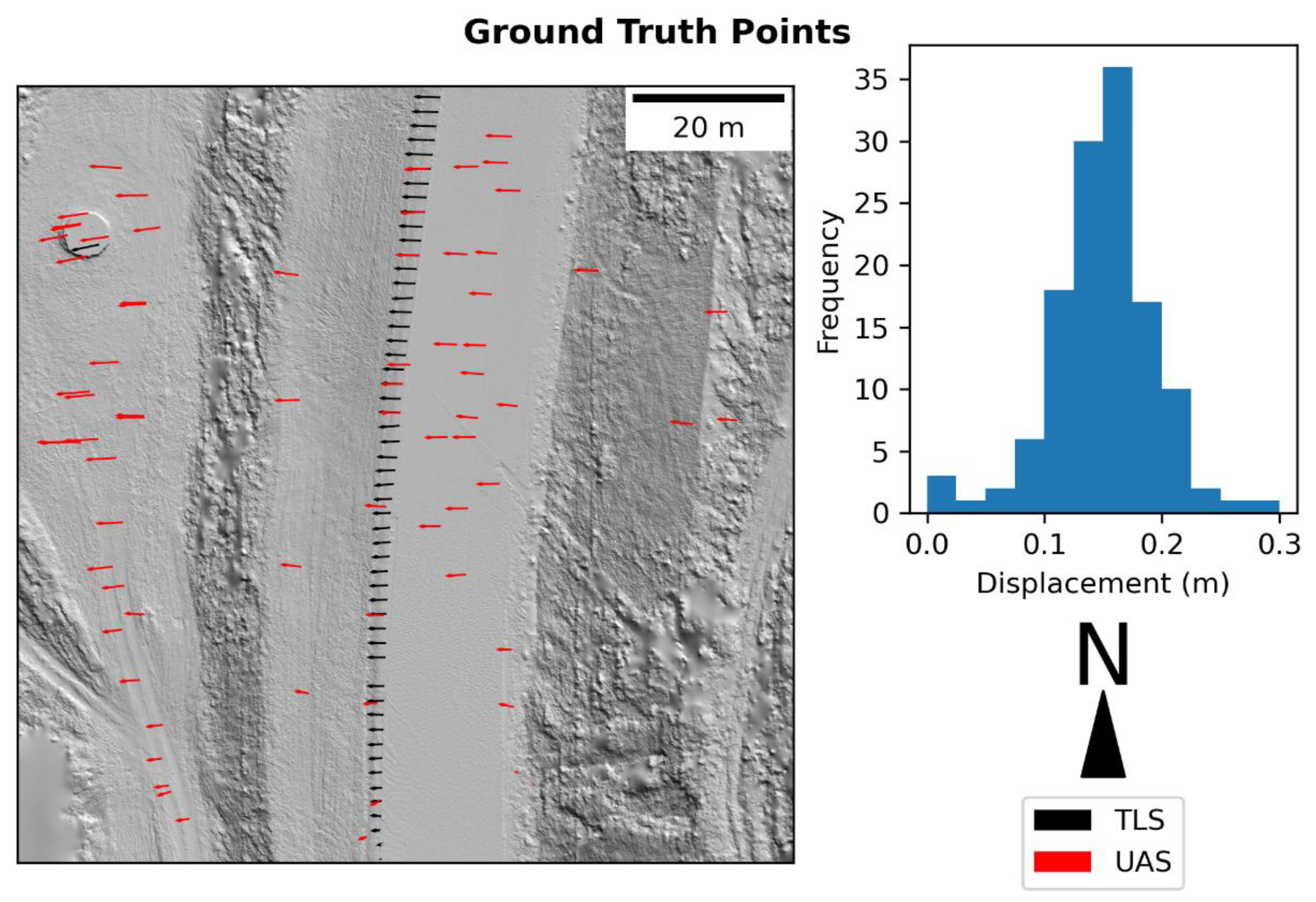
Displacements between two DEMs can be computed by performing inference on the trained model. Visual representations of the DEMs should be computed and fed into the model along with the optimized weight parameters computed during the training process, which will output a “flow” raster where each cell contains the predicted horizontal (u) and vertical (v) velocities between the two DEMs in image coordinates. These velocities can then be converted into real-word displacements by multiplying the image velocity components by the raster cell size as shown in Equations (7) and (8) below:

$$V_x=u\times \Delta X$$

(7)

$$V_y=v\times \Delta Y$$

(8)

where ΔX and ΔY are the x and y components of the cell size respectively. The vertical component of displacement is computed by using this 2D velocity grid to remap each cell of the post-landslide DEM to its original pre-displacement 2D position. Remapping of the post-landslide DEM is conducted for each cell by:

$$DE{M}_R\left(x,y\right)=DEM\left(x-u\left(x,y\right),y-v\left(x,y\right)\right)$$

(9)

where DEM_R is the remapped DEM, x and y are the raster coordinates and u and v are the x/y velocity grids in pixel coordinates. Interpolation can be used to compute the elevation value of pixels at non-integer raster coordinates. The actual vertical component of displacement can then be calculated by computing the per cell difference of the pre-landslide DEM from DEM_R. By combining this vertical displacement with the previously computed horizontal displacement, the actual 3D displacement that has occurred is computed across the landslide.

2.4. Test Dataset

The Arizona Inn Landslide (Figure 2) is situated approximately 23 km north of the city of Gold Beach between Highway 101 Mileposts 315 and 316 on the Southern Oregon Coast, USA. The landslide faces west with an average slope of approximately 20°. The primary area of interest is approximately 500 m wide (from north to south) and approximately 550 in length (from east to west). Like many coastal landslides, Arizona Inn is fronted by a steep coastal bluff approximately 50 m in height. At the top of the bluff is a relatively gentle bench traversed by Hwy 101. East of Hwy 101, the landslide extends upslope covering a steep, sparsely-vegetated slope approximately 120 m in height. In recent years, landslide movements have varied approximately 0.2 m to 0.3 m per year in the most active section just west of the highway [43].

A sequential set of surveys collected in the summers of 2020 and 2021 at the Arizona Inn Landslide were used to test the proposed approach. Data for each survey consisted of TLS scans collected with a Riegl VZ-400, and UAS SfM MVS photogrammetric dataset collected with a DJI Phantom 4 Pro RTK. Three Leica GS14 receivers were used during the survey: one to measure the location of each TLS scan position, another to measure GCP (ground control points) used for registration of the UAS data, and a third was setup as a local base station to enable post-processing. The TLS and UAS SfM datasets were processed and analyzed separately in order to demonstrate the performance and versatility of SlideSim. Each data source was individually georeferenced. TLS data were georeferenced using the approach outlined in [17,44] using the GNSS data to constrain the origin of each scan position. UAS SfM/MVS data were georeferenced using AgiSoft Metashape [45] using PPK processing conducted with rtklib [46] to constrain the UAS camera origins along with the GNSS measured GCP points as additional constraints. An approximate estimate of georeferencing accuracy for each data source was derived by computing the RMSE between corresponding points across the survey epochs on stable areas outside of the landslide extents. This yielded a 3D georeferencing RMSE of 0.008 m and 0.027 m between the two survey epochs for the TLS and UAS datasets, respectively. Ground filtering of the point cloud, generation of DEM rasters based on the median elevation value of the ground points for each cell in the XY plane, and hole-filling using a thin plate spline for interpolation in areas of the dataset with lower point density was performed as outlined in [47] to produce a continuous DEM for each data source/survey epoch.

For the quantitative assessment of SlideSim, a 10,486 m² subsection representing a 102.4 m by 102.4 m square of the landslide in the south-west portion of the landslide was used (Figure 3). This subsection was chosen because it contained:

• The highest point density of the TLS scans, enabling DEMs of several cell sizes to be created in order to properly assess the impact of cell size in the quality of the output displacement vectors as well as enabling the generation of high-quality ground truth points.
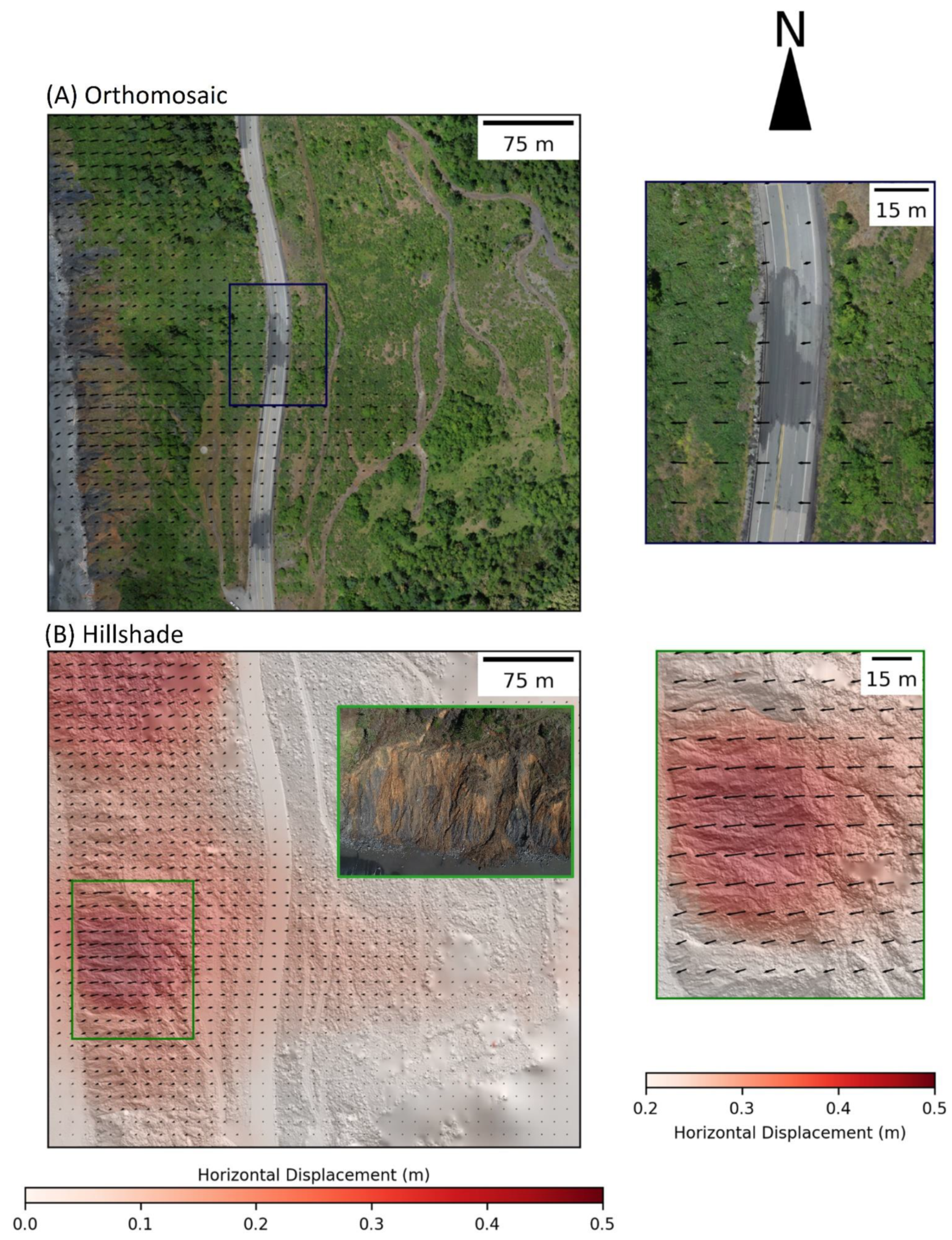
• A wide range of displacement magnitudes as it extends over a lateral scarp of one of the nested failures within the active portion of the landslide complex, and
• A wide variety of land cover types, ranging from west to east through: grass, sparse vegetation, paved road, and a patch of dense vegetation in the southeast (Figure 2).

For the quantitative assessment, the TLS derived datasets (

Table 2. Summary table describing each of the DEM rasters included in the test dataset.

Collection Date	Data Source	Cell Sizes (Δcell, m)	Extent Area (m2)	# of pts (million)	Mean pt Density (pts/0.01 m2)	Std Dev. pt Density (pts/0.01 m2)
06/14/2020	TLS	0.025, 0.05, 0.1, 0.2	10,485.76	30	29.3	176
	UAS	0.1	167,772.16	278	20.5	12.9
06/14/2021	TLS	0.025, 0.05, 0.1, 0.2	10,485.76	26	21	49.2
	UAS	0.1	167,772.16	176	15.8	10.3

) were used for each of the experiments, while the UAS derived dataset (Table 2) was used in the data source flexibility experiment.

2.5. Assessment of Accuracy

Performance of a rigorous accuracy assessment is important to measure the efficacy of a given approach. However, robustly assessing accuracy using data from a real-world landslide is more challenging than synthetically generated data where the correct results can be absolutely known. Challenges arise from multiple factors including: georeferencing uncertainty within the input datasets, artifacts present in the data, and the uncertainties involved in any method used to measure 3D landslide displacement.

For this study, a ground truth dataset of real-world 3D landslide displacement vectors was created using a combination of the georeferenced TLS point clouds and georeferenced orthomosaic images, which were collected at approximately the same time. The ground truth points from each of these data sources were combined and used for the assessment of all experiments shown below.

3D displacement vectors were created from the TLS point cloud data by extracting points within a given 2 m window around a unique object. At this particular site, guard rail posts and a drainage cistern were used as they were the only readily identifiable, consistent, and unique objects present across both survey epochs. Points located within these windows were then matched between the two survey epochs using an adapted ICP approach, similar to that used by [48], where the rotation angles were held constant to allow adjustment in translation only. Displacement vectors were then mapped to the coordinates of the center of the window. To ensure consistency, these displacement vectors were then verified manually by picking points between the two survey epochs.

Additional 3D displacement vectors were created from the UAS RGB orthomosaic images by manually matching pixels between common image features across the two datasets, enabling more geographically distributed points to be created. The vertical change component was computed using the DEMs where the vertical displacement was the elevation at the pixel in post landslide DEM minus the elevation at the matching pixel in the pre-landslide DEM.

In order to compare this ground truth to the output of SlideSim, a suitable method of assessing the accuracy of continuous finite grids should be used. In predictive optical flow, the most common method is the Endpoint Error (EPE) [49], which is calculated as the element-wise Euclidean distance between the vectors of the predicted and ground truth datasets as shown for the 2D and 3D cases in Equations (10) and (11), respectively:

$$EP{E}_{2D}=\sqrt{{\left(x_{gt}-x_{pred}\right)}^2+{\left(y_{gt}-y_{pred}\right)}^2}$$

(10)

$$EP{E}_{3D}=\sqrt{{\left(x_{gt}-x_{pred}\right)}^2+{\left(y_{gt}-y_{pred}\right)}^2+{\left(z_{gt}-z_{pred}\right)}^2}$$

(11)

where x_gt, y_gt, and z_gt are the ground truth 3D displacement vectors and x_pred, y_pred, and z_pred are the predicted 3D displacement vectors. The EPE is a measure of the total error across the predicted 3D displacement vector grid. High values indicate erroneous prediction, while low values indicate correct prediction.

2.6. Experiments

In order to test the efficacy of SlideSim for landslide displacement mapping, five different experiments were performed to evaluate and highlight various aspects of SlideSim. The experiments performed and their reasoning are highlighted in the sections below:

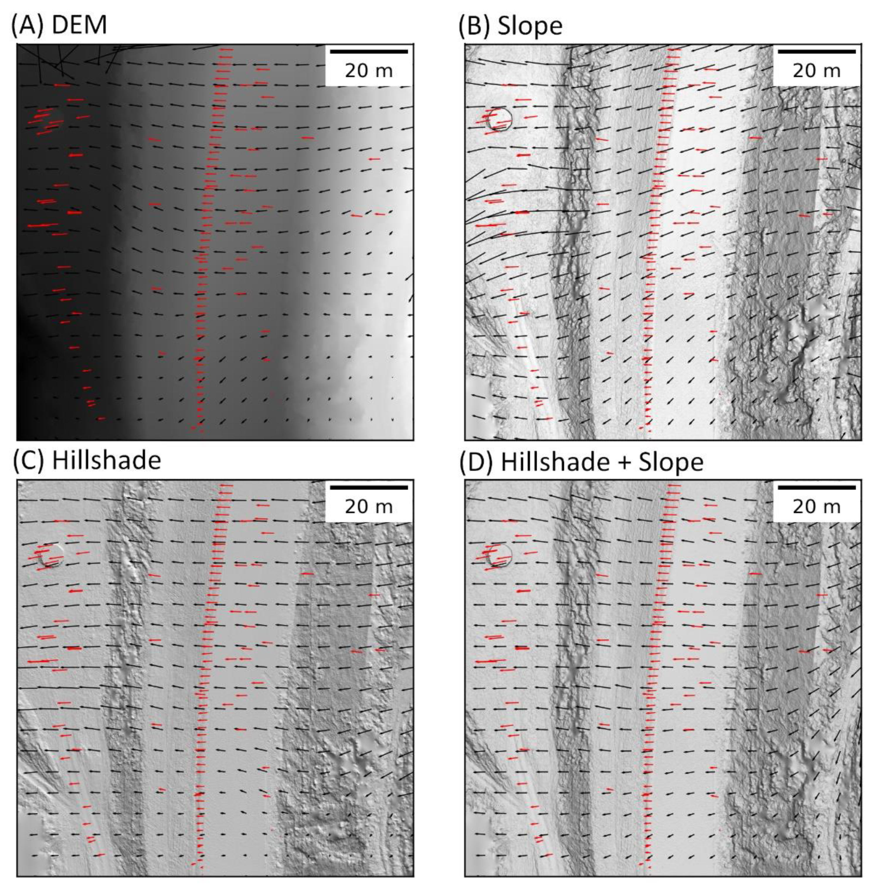
2.6.1. Experiment #1: Representation of DEM

DEMs contain raw elevation information over a given area. Since DEMs in their raw form are difficult to visualize in 2D, users are reliant on visual representations of the DEMs when performing any delineation or matching tasks using DEMs. These visual representations enhance contrast, delineate topographic features, and allow for overall easier visual perception and interpretation of the terrain. Rather than solely training the optical flow predictor model with the raw DEM, additional models are trained using visual representations since it is reasoned that these would make greater use of the pre-training on RGB images as well as provide a more flexible final model that is more likely to produce accurate results across a variety of terrain types.

In order to test the impact of DEM representation on model performance, four different optical flow predictor models were trained: the raw DEM, a hillshade representation of the DEM, a 3 × 3 slope map representation of the DEM, and a hybrid image containing each of the above in a separate band. Each were normalized to a range of 0 to 1. Both the hillshade and slope rasters were computed using a gradient approximation method [50] with a sliding 3 × 3 window. Each model was trained for 50 k iterations, and then inference was performed on the trained model and compared to the ground truth dataset created above.

2.6.2. Experiment #2: Cell Size of Input Model

Cell size (Δcell) is an important consideration when conducting any raster-based analysis [51,52]. A smaller Δcell enables the analysis to be conducted at a higher resolution so that smaller scale features can be considered within the analysis. However, this added information and detail comes at the expense of increased computational time as well as potential increased noise within the data. In change analysis, the optimal Δcell of input data requires careful consideration of both the quality of the input datasets as well as the scale of the change that has taken place.

To evaluate the sensitivity of model performance to the Δcell, four different models were trained using 0.025, 0.05, 0.1, and 0.2 m Δcell using the TLS DEM. Each model was trained for 50 k iterations using the hillshade representation of the DEM. Inference was then performed on the trained model and compared to the ground truth dataset created above.

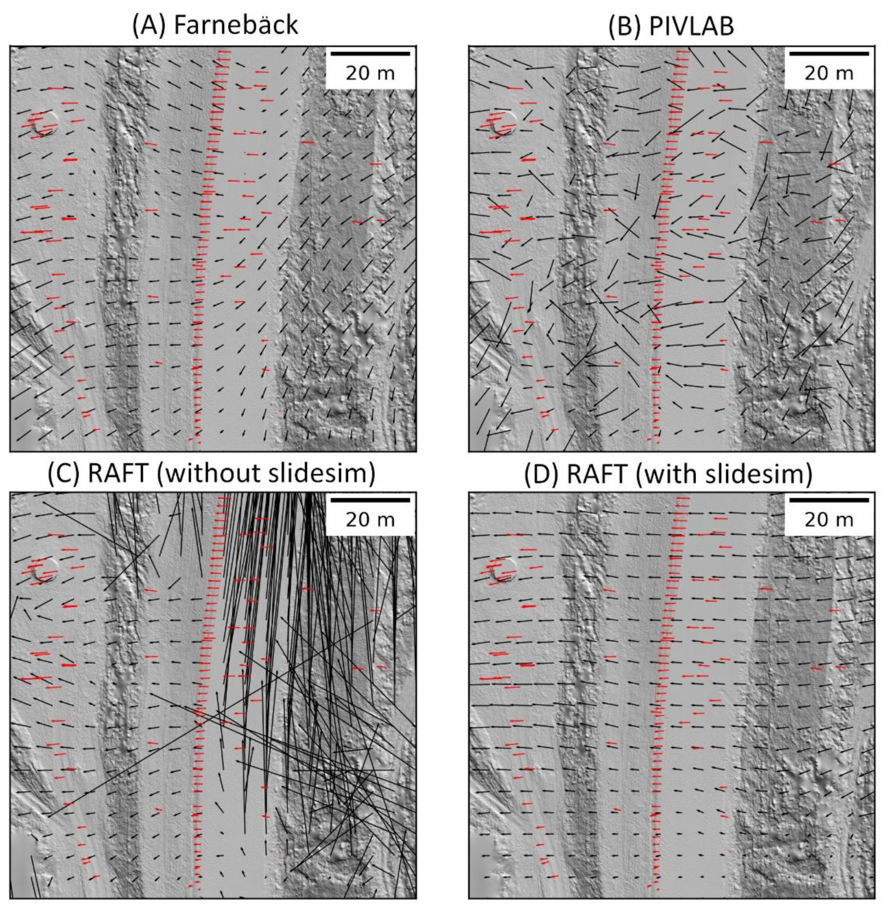
2.6.3. Experiment #3: Comparison to Other Methods

To show the effectiveness of the SlideSim methodology, three alternative methods were used to compute the horizontal displacement using a hillshade representation of the DEM. The accuracy of SlideSim was compared to these alternate published methods using the ground truth dataset in order to compare a wide range of approaches:

• The OpenCV implementation of Farnebäck optical flow algorithm [53], which is widely used to compute dense optical flow.
• The PIVlab [54] implementation of PIV (Particle Image Velocimetry), which has recently been used to compute horizontal displacement of geomorphological features using DEM derived products [27,55].
• The RAFT deep learning optical flow approach [10] in its typical implementation without additional training using SlideSim, providing a comparison to one of the most widely used deep learning based optical flow approaches trained solely on RGB images without additional landslide context.

2.6.4. Experiment #4: Vertical Component

One of the benefits of SlideSim is that it allows for the actual vertical component of change for a specific feature to be computed, resulting in full 3D mapping of displacements across the landslide. A typical change grid, in contrast, computes the vertical difference of subsequent DEMs without any consideration of the horizontal displacement. The proposed method evaluates the horizontal and vertical change simultaneously given that it is extracting vectors rather than simply differencing pixels. The accuracy of computed vertical change from the proposed, remapping method and a typical difference grid were compared using the ground-truth dataset.

2.6.5. Experiment #5: Data Source Flexibility

To test the versatility of this approach, SlideSim was also tested on a set of DEMs derived from UAS SfM MVS photogrammetric data collected at the same landslide site, in parallel with the TLS data. UAS is often advantageous for large landslide sites because it is more feasible to cover large areas compared with terrestrial based systems. DEMs (Δcell = 0.1 m) were created over a larger extent of the landslide in order to evaluate how this method could practically be applied to map the overall displacements across a large landslide. A separate optical flow predictor model was trained using the UAS derived DEM with SlideSim over the full extents using the same approach and parameter set as used for the TLS derived data above. The same ground truth dataset was also used in addition to test the accuracy of the 2D displacement predicted by inference of the trained model to the TLS derived data.

3. Results

3.1. Experiment #1: Representation of DEM

Table 3. 2D Accuracy of the proposed method using several representations of the DEM to compute landslide displacement reported as EPE (end-point error) in meters compared to ground truth points.

EPE Statistic	DEM	Slope	Hillshade	Hillshade + Slope
Min (m)	0.003	0.016	0.001	0.002
Max (m)	0.088	0.250	0.099	0.195
Mean (m)	0.035	0.086	0.021	0.029
Std. Dev. (m)	0.023	0.036	0.015	0.025
RMSE (m)	0.042	0.095	0.026	0.038

presents the 2D accuracy statistics of each of the DEM representation methods used, while Figure 4 shows a visualization of the results. The hillshade map produced the most accurate displacement vectors (EPE RMSE = 0.026 m) after model training. The hillshade/slope hybrid map and the normalized DEM map produced reasonable results overall (EPE RMSE = 0.038 m and EPE RMSE = 0.042 m, respectively). The slope map produced the least accurate displacement vectors overall (EPE RMSE = 0.095 m).

3.2. Experiment #2: Cell Size of Input Model

Table 4. 2D Accuracy of SlideSim using various cell sizes (Δcell) of the input model to compute landslide displacement reported as EPE (end-point error) in meters compared to ground truth points.

EPE Statistic	Δcell = 0.025 m	Δcell = 0.05 m	Δcell = 0.1 m	Δcell = 0.2 m
Min (m)	0.005	0.001	0.004	0.039
Max (m)	0.128	0.099	0.110	0.139
Mean (m)	0.036	0.021	0.046	0.079
Std. Dev. (m)	0.019	0.015	0.023	0.019
RMSE (m)	0.041	0.026	0.052	0.081

presents the final 2D accuracy statistics of the model trained/tested using the proposed method for each of the tested cell sizes. Overall, higher resolution (smaller cell size) models tend to perform much better than the lower resolution models (e.g., EPE RMSE = 0.026 m for Δcell = 0.05 m vs. 0.081 m for Δcell = 0.20 m). Figure 5 shows the EPE against the observed displacement in the ground truth dataset. Both the 0.1 m and 0.2 m models produced relatively high EPE for small displacements (<0.1 m), with EPE reducing as the magnitude of observed displacement increases. These results indicate slight trends with R² values of 0.47 and 0.26 for the 0.1 m and 0.2 m Δcell models respectively. EPE in the smaller Δcell models (0.025 m and 0.05 m) showed no trend, each with R² values of 0.05.

3.3. Experiment #3: Comparison to Other Methods

Table 5. 2D Accuracy of select approaches to compute landslide displacement reported as EPE (end point error) in meters compared to ground truth points.

EPE Statistic	Farnebäck Optical Flow	PIVLAB	RAFT (Without SlideSim)	RAFT (With SlideSim)
Min (m)	0.009	0.005	0.003	0.001
Max (m)	0.182	0.509	12.422	0.099
Mean (m)	0.070	0.112	3.071	0.021
Std. Dev. (m)	0.040	0.088	4.536	0.015
RMSE (m)	0.080	0.142	5.463	0.026

presents the final 2D accuracy statistics of each of the assessed methods. In addition to producing the most accurate results compared to the ground truth (EPE RMSE = 0.026 m), SlideSim also predicts the horizontal displacement geographically consistent with the ground truth across the whole test site (EPE standard deviation = 0.015 m) (Figure 6D). In comparison, some of the other methods worked well in areas of the test site but did not produce consistent results across the whole site (EPE RMSE = 0.080 m, 0.142 m, and 5.463 m for the Farnebäck, PIVlab, and RAFT without SlideSim, respectively).

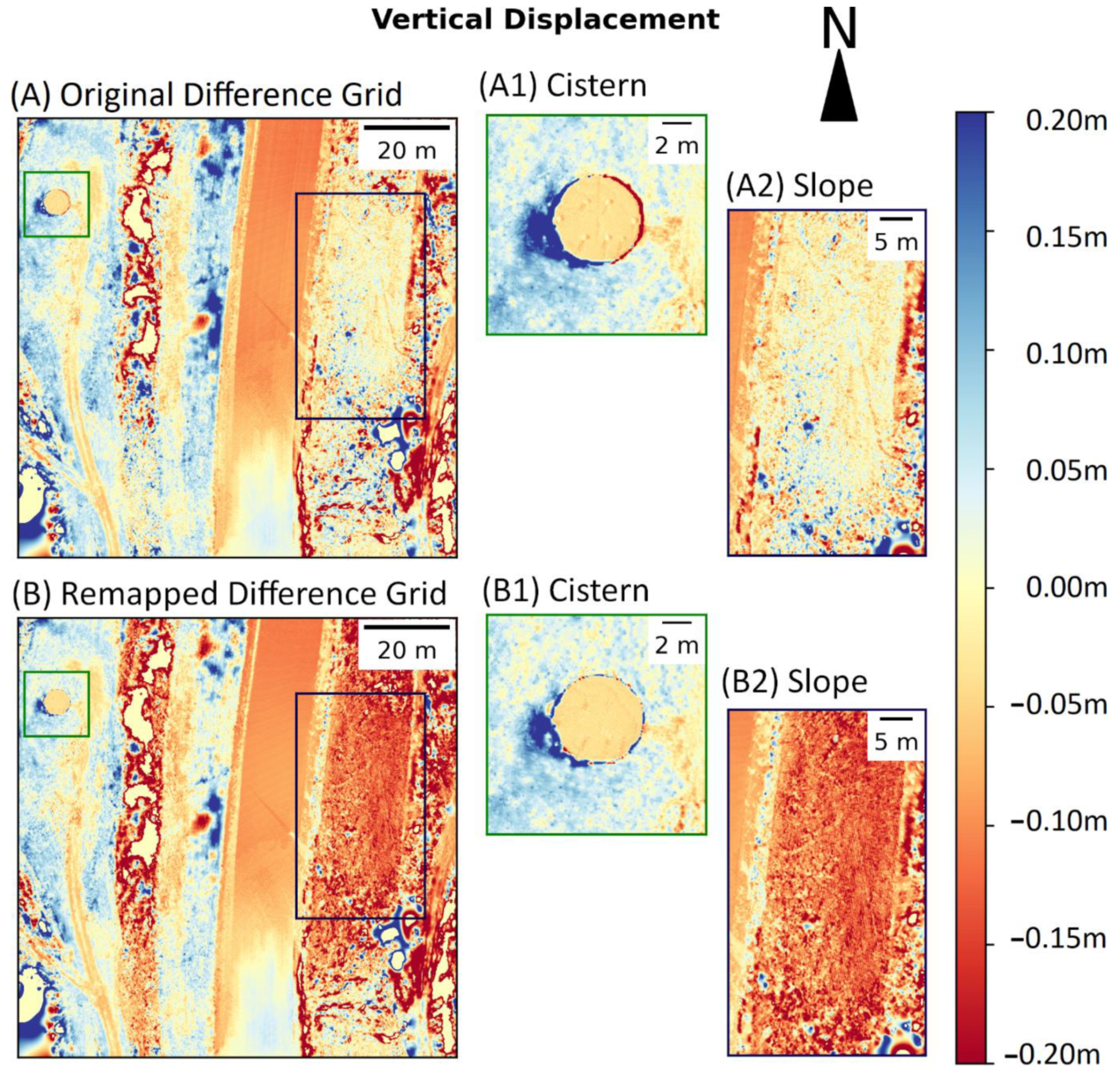
3.4. Experiment #4: Vertical Component

By remapping the DEMs using the horizontal displacement the RMSE improves significantly from 0.068 m to 0.007 m (

Table 6. Vertical accuracy of computing the vertical difference grid with and without using the proposed remapping approach, reported as the difference in meters compared to the ground truth.

EPE Statistic	Original Difference Grid	Remapped Difference Grid
Min (m)	−0.124	−0.031
Max (m)	0.692	0.038
Mean (m)	−0.001	0.001
Std. Dev. (m)	0.068	0.007
RMSE (m)	0.068	0.007

). Beyond the statistics, the difference between the two methods can more easily be observed by visualizing the computed vertical change across the landslide extents (Figure 7). In relatively flat areas (low slope) the estimated vertical change is very similar between the two methods. This can be observed by looking at the vertical change along the road for each method (Figure 7). However, in areas of the landslide with steep slopes, the estimated vertical change is very different between the two methods. This improvement is most readily observed in the test dataset by looking at the cistern west of the road and the slope immediately east of the road (Figure 7). This example shows that in areas where the slope aspect matches the direction of horizontal displacement (most common in a landslide), differencing the DEMs without accounting for horizontal change results in a positive (upward) bias in vertical displacement, whilst slope aspect facing the opposite direction results in a negative (downward) bias in vertical displacement.

3.5. Experiment #5: Data Source Flexibility

The UAS derived data performed better (

Table 7. Horizontal accuracy of the proposed method evaluated using 0.1 m DEMs derived from UAS SfM MVS data collected in tandem with the TLS data across the same extents. Reported as EPE (end-point error) in meters compared to the ground truth.

EPE Statistic	UAS
Min (m)	0.002
Max (m)	0.084
Mean (m)	0.027
Std. Dev. (m)	0.015
RMSE (m)	0.030

) than the 0.1 m TLS derived data over the same extent (EPE RMSE = 0.030 m for UAS vs. 0.052 m for TLS). In addition, the predicted 2D displacements computed using the UAS derived DEMs aligns with many of the extents that can be observed in the broader landslide. Figure 8A shows that the predicted displacements align with repaving markings along the highway, where repaving has been performed due to lateral extension occurring at the scarp of the landslide. The displacement grid also captures a nested failure that occurs within the main landslide body (Figure 8B) in the bluff section of the landslide. In this section, accelerated displacements line up with the scarp extents that can be observed in the hillshade of the DEM.

4. Discussion

4.1. Experiment #1: Representation of DEM

The hillshade map combines both slope (magnitude) and aspect (direction) of the local topography to produce a high contrast visual map that is relatively constant across survey epochs. The detailed encoding of topographic information visually within a single image produced the most accurate displacement vectors with relatively high consistency across the site (Figure 4C). The hillshade/slope hybrid model, while producing good results overall, still produced some erroneous north–south displacement predictions (Figure 4D) and did not perform as well as the model trained with the hillshade alone.

The poor performance of the slope map is likely because the slope map only considers magnitude and not direction, therefore, not considering the actual curvature of the slope within the plan view, limiting the ability of the network to identify similar features. For example, along the road and gentle grass slope immediately west of the road in Figure 4B, the network erroneously predicts a southerly component to the landslide displacement because of the relatively constant slope values in the north–south direction, similar to the hillshade/slope hybrid model. The slope map also experiences similar problems in the relatively flat section in the center-west section of the landslide (Figure 4B), where contrast in slope values is low, leading to the network overpredicting the westward displacement.

The normalized DEM map, on the other hand, exhibits a significant performance improvement over the slope However, the DEM trained model is not as robust as the hillshade models and struggles to produce accurate predictions near the edge of the DEM (Figure 4A), particularly in the northwest portion where some noisy displacement vectors occur.

4.2. Experiment #2: Cell Size of Input Model

The improved performance by the high-resolution models is likely in part due to their ability to detect small displacements more accurately compared with the low-resolution models. The low-resolution models (0.1 m and 0.2 m) produced higher EPE for small displacements (<0.1 m) due to over-predicting the displacement. This observed relationship is likely due to these small displacements being smaller than Δcell increasing the difficulty for the model to make correct predictions. The lack of trend between EPE and the magnitude of displacement in the high resolution (0.025 m and 0.05 m) models suggests that noise is the dominant factor contributing to the EPE for these models.

The fact that the 0.025 m model does not outperform the 0.05 m model (e.g., EPE RMSE = 0.041 m for Δcell = 0.025 m vs. 0.026 m for Δcell = 0.05 m) indicates that the resolution cannot be increased from the limit of the original input data source (in this case, the TLS derived point cloud). Further increases in resolution only introduce noise and artifacts from the interpolation and reduce smoothing of the original data by averaging points within a cell to remove outlier points.

The training process should also be considered when selecting Δcell. For example, if using a 512 × 512 random crop of the DEM in training, this would be the equivalent of using 163.84 m², 655.36 m², 2,621.44 m², and 10,485.76 m² sections to train the model for Δcell = 0.025, 0.05, 0.1, and 0.2 m, respectively. Therefore, for small values of Δcell, the model will have to learn to map displacement using smaller geographic features compared to when using larger values. Certainly, the size of the crop area can be increased to use larger sections of the DEM; however, this will result in exponential increases in the processing time to train the model and the GPU RAM consumed during training, which can often be a limiting factor.

4.3. Experiment #3: Comparison to Other Methods

The RAFT model (without SlideSim) produced more reasonable results in the lower grassy section (west of the road) where texture is higher (EPE RMSE = 0.072 m); however, this model produced poor results along the road (where texture is low) as well as poor results east of the road in the vegetated section where noise is higher (Overall EPE RMSE = 5.463 m) (Figure 6C). The Farnebäck method (Figure 6A) also produced reasonable results immediately west of the road; however, it produced poor results along the road as well as overall erroneous displacements along the y-axis (north–south) due to the low contrast along the y-axis at this particular hillshade (Overall EPE RMSE = 0.08 m). The PIV method (Figure 6B) produced overall erroneous displacement vectors across the whole of the landslide (Overall EPE RMSE = 0.142 m) PIV is designed to detect high contrast particles within a scene with consistent pixel intensities; hence, it is not ideal for landslide DEMs where contrast is often relatively low in comparison.

4.4. Experiment #4: Vertical Component

Given that landslides can often occur in areas of relatively steep slopes, accounting for the horizontal displacement is an extremely important part of determining the actual vertical displacement that has occurred across a given landslide. In addition, while other ground movement phenomena, such as subsidence and rockslope erosion, occur approximately perpendicular to the ground/reference surface plane, landslide displacement occurs approximately parallel to the local shear surface and therefore can have a strong horizontal component of movement. If landslide displacements are analyzed with 2D grids, then correcting for movement parallel to the reference grid is essential for accurate monitoring. The proposed remapping method robustly computes these displacements at a high resolution.

4.5. Experiment #5: Data Source Flexibility

The improved performance of the UAS derived data compared to the TLS derived data is likely due to the greater spatial context provided by supplying data beyond the test extent boundaries. Unlike the TLS data, UAS SfM MVS data cannot be as effectively ground filtered due to the nature of passive sensing [56]. As a result, this versatility test also demonstrates the ability of the proposed method to perform well with the additional noise and vegetation present in the DEM. In addition to providing accurate estimates of 3D landslide displacement, the proposed method with SlideSim can also delineate the landslide boundaries as well as any nested failures, or other changes affecting the rate of landslide displacement.

4.6. Limitations and Future Work

It is worth noting that several important limitations of mapping landslide displacements with SlideSim exist. First, just as any analysis that relies on remote sensed data, the performance of SlideSim depends on the quality and accuracy of the input DEMs. Poorly georeferenced DEMs, or DEMs with insufficient resolution will result in inaccurate displacement maps and potentially misleading measurements. Second, SlideSim has been designed assuming rigid/semi-rigid displacement on landslides that have not been fully evacuated, and therefore does not include debris flows, or rockfall type landslide failures. While the Conservation of Mass approach used by SlideSim is capable of modelling a diverse set of kinematic landslide motions, future work may want to consider adapting our approach to include more complex landslide displacement phenomena, such as nested failures. Additionally, future work studying the impact of changes in the input DEM cell size should be considered. This would involve examining the relationship between optimal cell sizes and accuracy of input data, scale of movement, and the size of geospatial features across multiple landslide sides to develop key insights into the relation between each of the above factors.

5. Conclusions

This paper presents a novel method enabling end-to-end self-supervised learning of landslide displacement monitoring called SlideSim. SlideSim is an automated simulation approach that generates labeled pairs of displaced landslide DEMs using real-world data for training of deep learning models to evaluate displacement resulting from landslide surface movements. The proposed method was evaluated both quantitatively and qualitatively on a real-world landslide dataset using multiple input data sources, resulting in the following conclusions:

• Real world landslide displacements can be accurately measured across a set of DEMs using a deep learning model trained on synthetically generated data, demonstrating that the proposed method is capable of training a model to identify displacements that have occurred without signs of overtraining.
• SlideSim can be completed with relatively few intuitive parameters and requires no direct supervision or tuning of hyperparameters when performing inference with the model.
• A variety of representations of the DEM can be used during both training and inference of the model; however, the hillshade representation produced the highest quality and most consistent results.
• Production of an accurate and dense 2D horizontal displacement grid enables remapping of the elevation values within the DEM to compute the actual vertical displacement that has occurred, producing significantly more accurate results than conventional DEM differencing that do not account for horizontal displacement.
• The method is robust to the input data source used to generate the DEMs and the presence of vegetation artifacts within the DEM did not appear to negatively affect the performance of the method at measuring displacements.

References

1. Höfle, B.; Rutzinger, M. Topographic Airborne LiDAR in Geomorphology: A Technological Perspective. Z. Fur Geomorphol. Suppl. 2011, 55, 1–29. [Google Scholar] [CrossRef]
2. Zhang, J.; Lin, X. Advances in Fusion of Optical Imagery and LiDAR Point Cloud Applied to Photogrammetry and Remote Sensing. Int. J. Image Data Fusion 2017, 8, 1–31. [Google Scholar] [CrossRef]
3. Iglhaut, J.; Cabo, C.; Puliti, S.; Piermattei, L.; O’Connor, J.; Rosette, J. Structure from Motion Photogrammetry in Forestry: A Review. Curr. For. Rep. 2019, 5, 155–168. [Google Scholar] [CrossRef] [Green Version]
4. Jaboyedoff, M.; Oppikofer, T.; Abellán, A.; Derron, M.-H.; Loye, A.; Metzger, R.; Pedrazzini, A. Use of LIDAR in Landslide Investigations: A Review. Nat. Hazards 2012, 61, 5–28. [Google Scholar] [CrossRef] [Green Version]
5. Lucieer, A.; de Jong, S.M.; Turner, D. Mapping Landslide Displacements Using Structure from Motion (SfM) and Image Correlation of Multi-Temporal UAV Photography. Prog. Phys. Geogr. 2014, 38, 97–116. [Google Scholar] [CrossRef]
6. Jaboyedoff, M.; Derron, M.-H. Landslide Analysis Using Laser Scanners. In Developments in Earth Surface Processes; Elsevier: Amsterdam, The Netherlands, 2020; Volume 23, pp. 207–230. [Google Scholar]
7. Ilg, E.; Mayer, N.; Saikia, T.; Keuper, M.; Dosovitskiy, A.; Brox, T. Flownet 2.0: Evolution of Optical Flow Estimation with Deep Networks. In Proceedings of the IEEE Conference on Computer Vision and Pattern Recognition, Honolulu, HI, USA, 21–26 July 2017; pp. 2462–2470. [Google Scholar]
8. Ren, Z.; Yan, J.; Ni, B.; Liu, B.; Yang, X.; Zha, H. Unsupervised Deep Learning for Optical Flow Estimation. In Proceedings of the Thirty-First AAAI Conference on Artificial Intelligence, San Francisco, CA, USA, 4–9 February 2017. [Google Scholar]
9. Hur, J.; Roth, S. Optical Flow Estimation in the Deep Learning Age. In Modelling Human Motion; Springer: Berlin/Heidelberg, Germany, 2020; pp. 119–140. [Google Scholar]
10. Teed, Z.; Deng, J. Raft: Recurrent All-Pairs Field Transforms for Optical Flow. In Proceedings of the European Conference on Computer Vision, Glasgow, UK, 23–28 August 2020; Springer: Berlin/Heidelberg, Germany; pp. 402–419. [Google Scholar]
11. Gordon, S.; Lichti, D.; Stewart, M. Application of a High-Resolution, Ground-Based Laser Scanner for Deformation Measurements. In Proceedings of the 10th International FIG Symposium on Deformation Measurements, Orange, CA, USA, 19–22 March 2001; pp. 23–32. [Google Scholar]
12. Abellán, A.; Oppikofer, T.; Jaboyedoff, M.; Rosser, N.J.; Lim, M.; Lato, M.J. Terrestrial Laser Scanning of Rock Slope Instabilities. Earth Surf. Processes Landf. 2014, 39, 80–97. [Google Scholar] [CrossRef]
13. Telling, J.; Lyda, A.; Hartzell, P.; Glennie, C. Review of Earth Science Research Using Terrestrial Laser Scanning. Earth-Sci. Rev. 2017, 169, 35–68. [Google Scholar] [CrossRef] [Green Version]
14. Babbel, B.J.; Olsen, M.J.; Che, E.; Leshchinsky, B.A.; Simpson, C.; Dafni, J. Evaluation of Uncrewed Aircraft Systems’ Lidar Data Quality. ISPRS Int. J. Geo-Inf. 2019, 8, 532. [Google Scholar] [CrossRef] [Green Version]
15. Westoby, M.J.; Brasington, J.; Glasser, N.F.; Hambrey, M.J.; Reynolds, J.M. ‘Structure-from-Motion’Photogrammetry: A Low-Cost, Effective Tool for Geoscience Applications. Geomorphology 2012, 179, 300–314. [Google Scholar] [CrossRef] [Green Version]
16. Simpson, C.H. A Multivariate Comparison of Drone-Based Structure from Motion and Drone-Based Lidar for Dense Topographic Mapping Applications. 2018. Available online: https://ir.library.oregonstate.edu/concern/graduate_thesis_or_dissertations/q524jv207 (accessed on 4 April 2022).
17. Olsen, M.J.; Johnstone, E.; Driscoll, N.; Ashford, S.A.; Kuester, F. Terrestrial Laser Scanning of Extended Cliff Sections in Dynamic Environments: Parameter Analysis. J. Surv. Eng. 2009, 135, 161–169. [Google Scholar] [CrossRef]
18. Kumar Mishra, R.; Zhang, Y. A Review of Optical Imagery and Airborne Lidar Data Registration Methods. Open Remote Sens. J. 2012, 5, 54–63. [Google Scholar] [CrossRef] [Green Version]
19. El-Sheimy, N. Georeferencing Component of LiDAR Systems. In Topographic Laser Ranging and Scanning; CRC Press: Boca Raton, FL, USA, 2017; pp. 195–214. [Google Scholar]
20. Meng, X.; Currit, N.; Zhao, K. Ground Filtering Algorithms for Airborne LiDAR Data: A Review of Critical Issues. Remote Sens. 2010, 2, 833–860. [Google Scholar] [CrossRef] [Green Version]
21. Che, E.; Senogles, A.; Olsen, M.J. Vo-SmoG: A Versatile, Smooth Segment-Based Ground Filter for Point Clouds via Multi-Scale Voxelization. ISPRS Ann. Photogramm. Remote Sens. Spat. Inf. Sci. 2021, 8, 59–66. [Google Scholar] [CrossRef]
22. Olsen, M.J.; Wartman, J.; McAlister, M.; Mahmoudabadi, H.; O’Banion, M.S.; Dunham, L.; Cunningham, K. To Fill or Not to Fill: Sensitivity Analysis of the Influence of Resolution and Hole Filling on Point Cloud Surface Modeling and Individual Rockfall Event Detection. Remote Sens. 2015, 7, 12103–12134. [Google Scholar] [CrossRef] [Green Version]
23. Bitelli, G.; Dubbini, M.; Zanutta, A. Terrestrial Laser Scanning and Digital Photogrammetry Techniques to Monitor Landslide Bodies. Int. Arch. Photogramm. Remote Sens. Spat. Inf. Sci. 2004, 35, 246–251. [Google Scholar]
24. Conner, J.C.; Olsen, M.J. Automated Quantification of Distributed Landslide Movement Using Circular Tree Trunks Extracted from Terrestrial Laser Scan Data. Comput. Geosci. 2014, 67, 31–39. [Google Scholar] [CrossRef]
25. Pfeiffer, J.; Zieher, T.; Bremer, M.; Wichmann, V.; Rutzinger, M. Derivation of Three-Dimensional Displacement Vectors from Multi-Temporal Long-Range Terrestrial Laser Scanning at the Reissenschuh Landslide (Tyrol, Austria). Remote Sens. 2018, 10, 1688. [Google Scholar] [CrossRef] [Green Version]
26. Teza, G.; Galgaro, A.; Zaltron, N.; Genevois, R. Terrestrial Laser Scanner to Detect Landslide Displacement Fields: A New Approach. Int. J. Remote Sens. 2007, 28, 3425–3446. [Google Scholar] [CrossRef]
27. Telling, J.W.; Glennie, C.; Fountain, A.G.; Finnegan, D.C. Analyzing Glacier Surface Motion Using LiDAR Data. Remote Sens. 2017, 9, 283. [Google Scholar] [CrossRef] [Green Version]
28. Khan, M.W.; Dunning, S.; Bainbridge, R.; Martin, J.; Diaz-Moreno, A.; Torun, H.; Jin, N.; Woodward, J.; Lim, M. Low-Cost Automatic Slope Monitoring Using Vector Tracking Analyses on Live-Streamed Time-Lapse Imagery. Remote Sens. 2021, 13, 893. [Google Scholar] [CrossRef]
29. Antonello, M.; Gabrieli, F.; Cola, S.; Menegatti, E. Automated Landslide Monitoring through a Low-Cost Stereo Vision System. In Proceedings of the Workshop Popularize Artificial Intelligence at the 13th Conference of the Italian Association for Artificial Intelligence AIxIA, Turin, Italy, 5 December 2013; pp. 37–41. [Google Scholar]
30. Leprince, S.; Ayoub, F.; Klinger, Y.; Avouac, J.-P. Co-Registration of Optically Sensed Images and Correlation (COSI-Corr): An Operational Methodology for Ground Deformation Measurements. In Proceedings of the 2007 IEEE International Geoscience and Remote Sensing Symposium, Barcelona, Spain, 23–28 July 2007; pp. 1943–1946. [Google Scholar]
31. Suncar, O.E.; Rathje, E.M.; Buckley, S.M. Deformations of a Rapidly Moving Landslide from High-Resolution Optical Satellite Imagery. In Proceedings of the Geo-Congress 2013: Stability and Performance of Slopes and Embankments III, San Diego, CA, USA, 3–7 March 2013; pp. 269–278. [Google Scholar]
32. Martin, J.G.; Rathje, E.M. Lateral Spread Deformations from the 2010–2011 New Zealand Earthquakes Measured from Satellite Images and Optical Image Correlation. In Proceedings of the 10th National Conference in Earthquake Engineering, Anchorage, AK, USA, 21–25 July 2014. [Google Scholar]
33. Bickel, V.T.; Manconi, A.; Amann, F. Quantitative Assessment of Digital Image Correlation Methods to Detect and Monitor Surface Displacements of Large Slope Instabilities. Remote Sens. 2018, 10, 865. [Google Scholar] [CrossRef] [Green Version]
34. Butler, D.J.; Wulff, J.; Stanley, G.B.; Black, M.J. A Naturalistic Open Source Movie for Optical Flow Evaluation. In Proceedings of the European Conference on Computer Vision, Florence, Italy, 7–13 October 2012; Springer: Berlin/Heidelberg, Germany, 2012; pp. 611–625. [Google Scholar]
35. Dosovitskiy, A.; Fischer, P.; Ilg, E.; Hausser, P.; Hazirbas, C.; Golkov, V.; Van Der Smagt, P.; Cremers, D.; Brox, T. Flownet: Learning Optical Flow with Convolutional Networks. In Proceedings of the IEEE International Conference on Computer Vision, Santiago, Chile, 7–13 December 2015; pp. 2758–2766. [Google Scholar]
36. Booth, A.M.; Lamb, M.P.; Avouac, J.-P.; Delacourt, C. Landslide Velocity, Thickness, and Rheology from Remote Sensing: La Clapière Landslide, France. Geophys. Res. Lett. 2013, 40, 4299–4304. [Google Scholar] [CrossRef] [Green Version]
37. Bunn, M.; Leshchinsky, B.; Olsen, M.J. Estimates of Three-Dimensional Rupture Surface Geometry of Deep-Seated Landslides Using Landslide Inventories and High-Resolution Topographic Data. Geomorphology 2020, 367, 107332. [Google Scholar] [CrossRef]
38. Mayer, N.; Ilg, E.; Hausser, P.; Fischer, P.; Cremers, D.; Dosovitskiy, A.; Brox, T. A Large Dataset to Train Convolutional Networks for Disparity, Optical Flow, and Scene Flow Estimation. In Proceedings of the IEEE Conference on Computer Vision and Pattern Recognition, Las Vegas, NV, USA, 27–30 June 2016; pp. 4040–4048. [Google Scholar]
39. Senogles, A. Slidepy: A Fast Multi-Threaded Python Library for 3D Landslide Modeling with SIMD Support. 2022. Available online: https://zenodo.org/record/6350744#.Ypgrv-xByMo (accessed on 4 April 2022).
40. Senogles, A. Fasterraster: A Fast Multi-Threaded Python Library for Performing Raster Operations with Simple IO. 2022. Available online: https://zenodo.org/record/6350746#.Ypgr6exByMo (accessed on 4 April 2022).
41. Smith, L.N.; Topin, N. Super-Convergence: Very Fast Training of Neural Networks Using Large Learning Rates. In International Society for Optics and Photonics, Proceedings of the Artificial Intelligence and Machine Learning for Multi-Domain Operations Applications, Bellingham, WA, USA, 10 May 2019; International Society for Optics and Photonics, SPIE: Bellingham, WA, USA, 2019; Volume 11006, p. 1100612. [Google Scholar]
42. Paszke, A.; Gross, S.; Massa, F.; Lerer, A.; Bradbury, J.; Chanan, G.; Killeen, T.; Lin, Z.; Gimelshein, N.; Antiga, L.; et al. Pytorch: An Imperative Style, High-Performance Deep Learning Library. In Proceedings of the 33rd Conference on Neural Information Processing Systems (NeurIPS2019), Vancouver, Canada, 8–14 December 2019; Volume 32, pp. 8024–8035. Available online: https://proceedings.neurips.cc/paper/2019/file/bdbca288fee7f92f2bfa9f7012727740-Paper.pdf (accessed on 4 April 2022).
43. Olsen, M.J.; Leshchinsky, B.; Senogles, A.; Allan, J. Coastal Landslide and Sea Cliff Retreat Monitoring for Climate Change Adaptation and Targeted Risk Assessment. SPR807 Interim Report; Oregon Department of Transportation: Salem, OR, USA, 2020.
44. Olsen, M.J.; Johnstone, E.; Kuester, F.; Driscoll, N.; Ashford, S.A. New Automated Point-Cloud Alignment for Ground-Based Light Detection and Ranging Data of Long Coastal Sections. J. Surv. Eng. 2011, 137, 14–25. [Google Scholar] [CrossRef]
45. AgiSoft Metashape Professional, Version 1.7.2. 2021. Available online: https://www.agisoft.com/ (accessed on 4 April 2022).
46. Takasu, T.; Yasuda, A. Development of the Low-Cost RTK-GPS Receiver with an Open Source Program Package RTKLIB. In Proceedings of the International Symposium on GPS/GNSS, Jeju, Korea, 4–6 November 2009; International Convention Center: Jeju, Korea, 2009; Volume 1. [Google Scholar]
47. Olsen, M.; Massey, C.; Leschinsky, B.; Senogles, A.; Wartman, J. Predicting Seismic-Induced Rockfall Hazard for Targeted Site Mitigation; FHWA-OR-RD-21-06; Oregon Department of Transportation: Salem, OR, USA, 2020. Available online: https://www.oregon.gov/odot/Programs/ResearchDocuments/SPR809RockFall.pdf (accessed on 4 April 2022).
48. Nissen, E.; Krishnan, A.K.; Arrowsmith, J.R.; Saripalli, S. Three-Dimensional Surface Displacements and Rotations from Differencing Pre-and Post-Earthquake LiDAR Point Clouds. Geophys. Res. Lett. 2012, 39. [Google Scholar] [CrossRef]
49. Otte, M.; Nagel, H.-H. Optical Flow Estimation: Advances and Comparisons. In Proceedings of the European Conference on Computer Vision, Stockholm, Sweden, 2–6 May 1994; Springer: Berlin/Heidelberg, Germany, 1994; pp. 49–60. [Google Scholar]
50. Zevenbergen, L.W.; Thorne, C.R. Quantitative Analysis of Land Surface Topography. Earth Surf. Processes Landf. 1987, 12, 47–56. [Google Scholar] [CrossRef]
51. Ziadat, F.M. Effect of Contour Intervals and Grid Cell Size on the Accuracy of DEMs and Slope Derivatives. Trans. GIS 2007, 11, 67–81. [Google Scholar] [CrossRef]
52. Yang, P.; Ames, D.P.; Fonseca, A.; Anderson, D.; Shrestha, R.; Glenn, N.F.; Cao, Y. What Is the Effect of LiDAR-Derived DEM Resolution on Large-Scale Watershed Model Results? Environ. Model. Softw. 2014, 58, 48–57. [Google Scholar] [CrossRef]
53. Farnebäck, G. Two-Frame Motion Estimation Based on Polynomial Expansion. In Proceedings of the Scandinavian Conference on Image Analysis, Norrköping, Sweden, 11–13 June 2003; Springer: Berlin/Heidelberg, Germany; pp. 363–370. [Google Scholar]
54. Thielicke, W.; Stamhuis, E. PIVlab–towards User-Friendly, Affordable and Accurate Digital Particle Image Velocimetry in MATLAB. J. Open Res. Softw. 2014, 2, e30. [Google Scholar] [CrossRef] [Green Version]
55. Reinoso, J.F.; León, C.; Mataix, J. Estimating Horizontal Displacement between DEMs by Means of Particle Image Velocimetry Techniques. Remote Sens. 2016, 8, 14. [Google Scholar] [CrossRef] [Green Version]
56. Eltner, A.; Kaiser, A.; Castillo, C.; Rock, G.; Neugirg, F.; Abellán, A. Image-Based Surface Reconstruction in Geomorphometry–Merits, Limits and Developments. Earth Surf. Dyn. 2016, 4, 359–389. [Google Scholar] [CrossRef] [Green Version]
Figure 1. Examples of SlideSim augmentation, showing the augmentation of the original DEM for several velocity grid, landslide boundary, and slip surface combinations. The numbers of coarse grid points used to generate each of the velocity grids are 9, 16, 25, and 36 for rows 1, 2, 3, and N, respectively. Velocity vector magnitude/direction is indicated by quiver arrows (scaled 20×) as well as background color (blue = substantial movement, green/yellow = intermediate, purple = small).
Remotesensing 14 02644 g001
Figure 2. Overview map showing the Arizona Inn landslide complex and approximate boundaries, the section used for the quantitative analysis (TLS boundary), and the UAS data boundary.
Remotesensing 14 02644 g002
Figure 3. Ground truth points used within the quantitative analysis subsection of the landslide. Black vectors (54 total) were measured from the TLS point cloud using an adapted ICP approach. Red vectors (73 total) were measured from a set of georeferenced orthomosaic RGB images collected at the same time as the TLS surveys. Vectors are scaled 20×. Histogram shows the frequency of each magnitude of displacement bins.
Remotesensing 14 02644 g003
Figure 4. Visualization of the output 2D landslide displacement using 4 different DEM representations: (A) Normalized DEM, (B) Slope, (C) Hillshade, and (D) Combined Hillshade and slope. Black vectors show the output 2D displacement vectors plotted every 100 cells, while the red vectors show the ground truth vectors measured from the ground truth dataset. All vectors are scaled 20×.
Remotesensing 14 02644 g004
Figure 5. EPE vs. magnitude of displacement for four different input model cell sizes evaluated against the ground truth dataset.
Remotesensing 14 02644 g005
Figure 6. Visualization of 2D landslide displacement mapping using 4 different methods: (A) Farnebäck optical flow, (B) PIVLAB, (C) RAFT without SlideSim, and (D) RAFT with SlideSim. Black vectors show the predicted 2D displacement vectors plotted every 100 cells, while the red vectors show the ground truth vectors measured from the ground truth dataset. All vectors are scaled 20×.
Remotesensing 14 02644 g006
Figure 7. Vertical difference grid between DEMs from subsequent survey epochs from (A) a regular difference grid and (B) computed using the proposed remapping approach with close-up views of the cistern (#1) and hillslope (#2).
Remotesensing 14 02644 g007
Figure 8. Visualization of the Horizontal displacement computed using SlideSim on the UAS data over the larger extents. Vectors are scaled 20×.
Remotesensing 14 02644 g008