Article

Robust Space–Time Joint Sparse Processing Method with Airborne Active Array for Severely Inhomogeneous Clutter Suppression

1
College of Information and Communication, National University of Defense Technology, Wuhan 430035, China
2
Early Warning and Detection Department, Air Force Engineering University, Xi’an 710051, China
3
School of Computer Science and Technology, Xi’an Jiaotong University, Xi’an 710049, China
4
Shaanxi Key Laboratory of Intelligence Coordination Networks, Xi’an 710106, China
*
Author to whom correspondence should be addressed.
Remote Sens. 2022, 14(11), 2647; https://doi.org/10.3390/rs14112647
Submission received: 28 April 2022 / Revised: 27 May 2022 / Accepted: 30 May 2022 / Published: 1 June 2022

Abstract

:
Due to clutter inhomogeneity, the clutter suppression ability of space–time adaptive processing (STAP) is usually constrained by the insufficient number of independent and identically distributed (IID) clutter training samples and, as a result, is sacrificed to achieve the demanded sample reduction. Moreover, since clutter heterogeneity is exacerbated in the real environment, the IID training sample size can be heavily reduced, leading to the deterioration in clutter suppression. To solve this problem, a novel robust space–time joint sparse processing method with airborne active array is proposed. This method has several outstanding advantages: (1) only the single snapshot cell under test (CUT) data is used for the superior clutter suppression performance; and (2) the proposed method completely removes the dependence of the system processing ability on IID training samples. In this paper, the signal model of uniform transmitting subarray diversity is first established to obtain the single snapshot echo observed CUT data. Then, with the matched reconstruction, the single snapshot data are equivalently converted into multi-frame echo data. Finally, a fast multi-frame echo data joint sparse Bayesian algorithm is used to achieve heterogeneous clutter suppression. Numerous experiments were performed to verify the advantages of the proposed method.

Graphical Abstract

1. Introduction

Low-altitude moving-target detection with airborne radar in a highly cluttered ground environment is currently a popular research topic. In the process of target detection using airborne radar, the relative position between the radar and ground clutter is changed due to the motion of the airborne platform. Then, Doppler broadening is generated and the ground clutter shows an apparent space–time coupling property, leading to the submergence of the target in the ground clutter and the severe deterioration in the target detection performance. Related techniques have been used to suppress relative stationary clutter, such as moving target indication (MTI), moving target detection (MTD), and pulse Doppler (PD) [1,2,3]. However, the space–time coupling clutter problem cannot be solved effectively. For this purpose, a kind of space–time adaptive processing (STAP) technique has been proposed for clutter suppression [4,5,6]. In this technique, the space–time two-dimensional echo data are first obtained by different spatial channels and temporal pulses. Second, numerous training samples that are adjacent to the cell under test (CUT) are selected to estimate the clutter covariance matrix (CCM) of CUT. Third, the weights of space–time filtering are calculated and the clutter is suppressed. The performance of this technique mainly depends on the estimated accuracy of CCM. According to the Reed–Mallet–Brennan (RMB) criterion [7], to achieve approximately optimal performance, the training samples used to estimate CCM should be independent and identically distributed (IID) with respect to CUT, and the number of IID training samples should be at least twice as many as the degrees of freedom (DOFs) [8,9]. This condition can be satisfied when the airborne radar is in a homogeneous clutter environment. However, in actual clutter circumstances, significant heterogeneity emerges because of the inner movement of clutter, topographic variation, and some external factors. As a result, the IID relationship between training samples and CUT is not maintained [10]. This causes the number of IID samples to decrease rapidly, and the error of CCM estimation to increase. Finally, the clutter suppression performance of STAP is worsened.
To solve the problem of insufficient IID training sample size, many improved methods have been proposed from different perspectives, and can be generally divided into two categories. The first aims to reduce the demanded quantity of IID samples, and uses various measures such as designing the transformation matrix, building the parametric model, constructing the knowledge-aided detector, and representing the clutter sparsity so as to realize the minimized IID sample requirement in the actual treatment. Correspondingly, some representative methods are reduced-rank STAP (RR-STAP) [11,12], reduced-dimension STAP (RD-STAP) [13,14], parametric STAP [15,16], knowledge-aided STAP (KA-STAP) [17,18], sparse recovery STAP (SR-STAP) [19,20,21], and other modified algorithms [22,23,24]. The second category is known as the direct processing method, which estimates CCM only using CUT without considering the training samples. Similarly, some representative techniques are direct data domain STAP (D3-STAP), smoothing STAP, and other improved algorithms [25,26,27,28]. In accordance with the former approaches, the key idea is to weaken the limitation of the IID sample size. However, the clutter suppression performance is heavily dependent on the number and quality of IID samples, and it is difficult to remove the constraint on the training samples. As the complexity of the detection environment is further increased, the IID sample size required to achieve a favorable CCM estimation is difficult to satisfy. The required sample size may be achieved at the cost of sacrificing the system processing capacity, even if the number of IID samples is able to be reduced by the first approach. The latter approach, considering the greater difficulty of obtaining sufficient IID training samples, attempts to use CUT for STAP without directly training the whole sample. Nevertheless, some system degrees of freedom are wasted and clutter suppression performance is evidently reduced, even though the processing is not limited by the training samples.
Simultaneously, the variable status of the modern battlefield electromagnetic environment is complicated. Detecting a low-altitude target with airborne radar is not only influenced by the above factors, such as topographic modification, clutter motion, and meteorological conditions, but is also seriously challenged by the numerous artificial strong scattering targets, hostile intentional interference, and unrelated moving targets [29]. Therefore, the low-altitude detecting scene for airborne radar is frequently changeable and time varying. As a result, the inhomogeneity of the ground clutter is severely increased and the IID relation between training samples and CUT is dramatically affected. The system processing difficulty is further exacerbated, and the deterioration in clutter suppression performance is accordingly aggravated because of the extreme shortage of IID training samples [19]. Under the premise of maintaining the system processing capacity and removing the restriction in training samples, it is crucial to seek a novel approach to address the deleterious effects on the clutter suppression performance in a severely inhomogeneous environment.
In recent years, a new type of radar system—the airborne active array—was introduced and extensively studied by the radar community due to its inherent superiority [30,31,32]. Compared with the passive phased array radar, the airborne active array’s spatial selectivity can be evidently promoted. The airborne active array also has the abilities of flexible configuration between transmitting and receiving array elements, construction the transmitting and receiving multi-beams, and reasonable optimization of transmitted waveforms. As a result, this method provides greater potential for airborne radar clutter suppression [33,34]. To increase the transmitting spatial freedom degree, many means can be adopted in the airborne active array, such as orthogonal spatial diversity, subarray division, and subarray beamforming in the transmitting array [35,36]. In addition, many different combinatorial configurations between the transmitter and the receiver are structured, such as the mode of transmitting subarray diversity and the whole receiving element, the mode of transmitting subarray diversity and the partial receiving element, and the mode of transmitting subarray diversity and receiving subarray division. Based on these advantages, the various radar echo forms may be acquired, which allows additional aspects of the clutter suppression performance to be improved.
Therefore, this paper focuses on the problem that the ground clutter suppression and the low-altitude moving target detection are evidently damaged because of the extreme shortage of IID training samples in a severely inhomogeneous clutter environment. To address this issue, a novel, robust space–time joint sparse processing method with airborne active array is proposed. Specifically, with the aid of the special advantages of the airborne active array in the interference suppression and sparse Bayesian learning (SBL) framework [23], space–time joint sparse processing of the single snapshot CUT data is used to obtain an equivalent multi-frame sample of CUT and realize the effective estimation of CCM, regardless of the IID characteristic of the training samples. Moreover, the proposed method completely removes the dependence of many current techniques on training samples, overcomes the limitation of the training sample size and quantity on STAP processing, and avoids the influence of the sample inhomogeneity on clutter suppression performance. The specific processing used in the presented method is divided into four main steps.
(1)
Subarray division on the radar transmitter. The transmitting elements can be divided into several subarrays with the same number of elements in each subarray. In order to realize the spatial diversity of the transmitting subarrays, the orthogonal waveform signals are transmitted among different subarrays. Furthermore, the coherent waveform signal is transmitted within each subarray. In the case of this transmitting form, it can not only acquire the orthogonal transmitting waveform and reduce the dimension of the receiving data, but also utilize the directional gain and the coherence processing gain inside the transmitting subarray. Therefore, greater transmitting domain selectivity is provided for inhomogeneous clutter suppression.
(2)
Echo data acquisition of CUT. Multi-group echo data corresponding to different transmitting subarrays can be obtained by a single matched filter bank in each receiving element. Simultaneously, equivalent multi-frame echo data corresponding to all of the transmitting subarrays can be obtained in the whole receiving array.
(3)
Sparse spectrum calculation of CUT. Combined with a fast sparse Bayesian learning algorithm, the sparse spectrum of CUT is calculated by the joint sparse processing of the multi-frame echo data.
(4)
CCM estimation and clutter suppression. According to the approximate prior information of the target under test, it is removed from the sparse spectrum of CUT. Then, CCM is effectively estimated and the filtering weights are obtained.
The remainder of this paper is organized as follows. The signal model of the proposed method is established in Section 2. The robust space–time joint sparse processing method based on single snapshot echo observed data and SBL is presented in Section 3. Simulation experiments and analyses comparing the results with previous studies are shown to prove the feasibility and validity of the proposal in Section 4. The conclusions are drawn in Section 5.

2. Signal Model of Uniform Transmitting Subarray Diversity

Suppose that the airborne active side-looking array consists of M × N elements, where M and N denote the transmitting element size and the receiving element size, respectively. The transmitter is divided into W W < M uniform subarrays. There are G elements in each subarray and the transmitter satisfies W × G = M . d t , d r and d T w respectively represent the transmitting element interval inside the subarrays, the receiving element interval, and the phase center interval of the transmitting subarray w   ( w = 1 , 2 , , W ) . λ is the radar wavelength. T and K represent the pulse repetition interval (PRI) and the number of pulses in a coherent processing interval (CPI), respectively. v p and H denote the flight velocity and the height of the airborne plane, respectively. The orthogonal waveform signals γ 1 , , γ w , , γ W are transmitted among the different subarrays, and the coherent waveform signal is transmitted within each subarray. The spatial geometric relation of the airborne active side-looking array based on the transmitting subarray diversity is shown in Figure 1.
θ q and φ q are the azimuth and elevation angle of clutter patch χ q corresponding to the airborne active array, respectively. When the non-ideal error of the array antenna is not considered, χ q is irradiated by the transmitting signal γ w of the subarray w . During the pulse k   ( k = 1 , 2 , , K ) , the clutter scattering signal of χ q that is obtained by the matched processing of the receiving element n   ( n = 1 , 2 , , N ) can be denoted as [37]:
χ q c ( w , n , k ) = ζ q e j 2 π ( k 1 ) f d q e j 2 π ( n 1 ) f s r q i = 1 W γ w γ i * δ w q
where ζ q is the clutter scattering intensity, δ w q is the directional gain of the transmitting subarray w relative to the clutter patch χ q , and f d q , f s r q are the normalized Doppler frequency and receiving spatial frequency of χ q , respectively, which are defined as:
f d q = 2 v p T cos ( θ q ) cos ( φ q ) / λ
f s r q = d r cos ( θ q ) cos ( φ q ) / λ
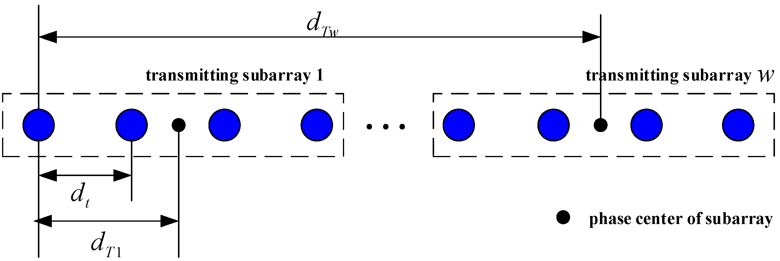
For better understanding of δ w q in Equation (1), the concept of phase center about the transmitting subarray needs to be explained. Its spatial structure is shown in Figure 2.
The phase center intervals of the transmitting subarray 1 and w are respectively denoted as d T 1 , d T w . Figure 2 shows that the phase center interval of the transmitting subarray w is expressed as:
d T w = d t w 1 G + 0.5 × ( G 1 ) , 1 w W
Then, the transmitting spatial frequency of χ q is derived as:
f s w q = d T w cos ( θ q ) cos ( φ q ) / λ
Considering that the synthetic beam shape of the transmitting subarray is influenced by the number of elements in each subarray, δ w q is expressed as [38]:
δ w q = c = 1 G exp j 2 π α f s r q z w + c 1 = exp j 2 π α f s r q z w × 1 exp j 2 π α f s r q G 1 exp j 2 π α f s r q = sin π α f s r q G sin π α f s r q × exp j 2 π α f s r q z w + G 1 / 2
where α = d t / d r , z w = w 1 G .
Furthermore, δ w q can be written as:
δ w q = sin ( π α f s r q G ) sin ( π α f s r q ) e j 2 π f s w q
In view of the waveform orthogonality among the transmitting subarrays, the different transmitting signals satisfy:
γ w γ i * = 1 , w = i γ w γ i * = 0 , w i
According to Equations (4)–(8), Equation (1) can be simplified as:
χ q c ( w , n , k ) = F ( f s r q ) ζ q e j 2 π ( k 1 ) f d q e j 2 π ( n 1 ) f s r q e j 2 π f s w q = F ( f s r q ) ζ q e j 2 π ( k 1 ) f d q e j 2 π ( n 1 ) f s r q e j 2 π d T w f s r q / d r
where F ( f s r q ) = sin ( π α f s r q G ) / sin ( π α f s r q ) , f s w q = d T w f s r q / d r .
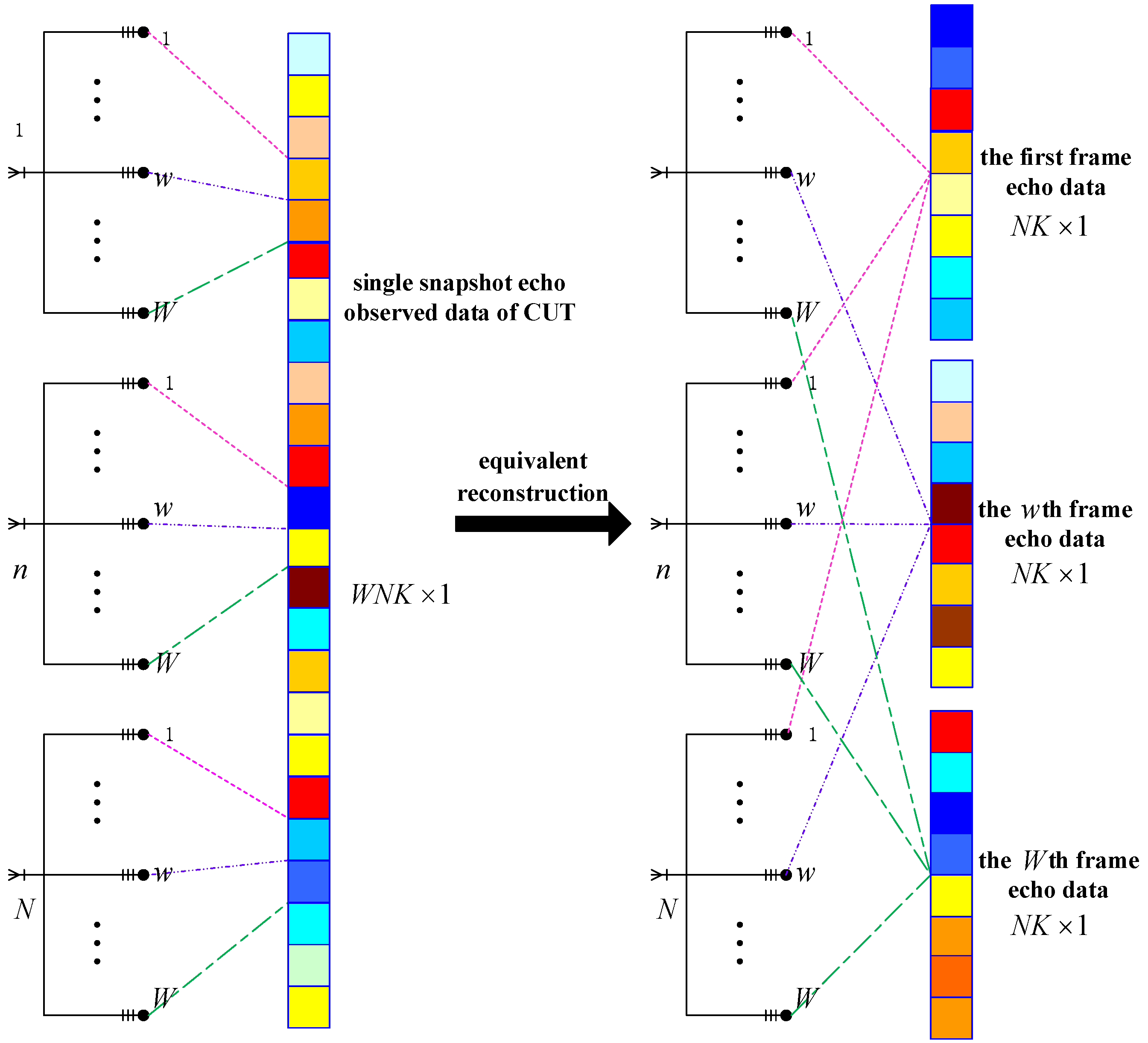
The echo data-acquiring schematic diagram of the airborne active array radar, considering the transmitting subarray diversity, is shown in Figure 3.
From Figure 3, it can be seen that, after the data are received by N elements, the single snapshot echo observed data of CUT are obtained and processed by the matched filters. The dimensions of the single snapshot observed data are W N K × 1 .
On the basis of Equation (9), the transmitting spatial steering vector, receiving spatial steering vector, and temporal steering vector of the clutter patch χ q are respectively defined as
S s t ( f s r q ) = F ( f s r q ) e j 2 π d T 1 f s r q / d r , F ( f s r q ) e j 2 π d T 2 f s r q / d r , , F ( f s r q ) e j 2 π d T W f s r q / d r T S s r ( f s r q ) = 1 , e j 2 π f s r q , , e j 2 π ( N 1 ) f s r q T S d ( f d q ) = 1 , e j 2 π f d q , , e j 2 π ( K 1 ) f d q T
Then, the echo data of χ q corresponding to the whole transmitting subarray are expressed as:
χ q c = ζ q S s t ( f s r q ) S s r ( f s r q ) S d ( f d q ) = ζ q F ( f s r q ) S ˜ s t ( f s r q ) S s r ( f s r q ) S d ( f d q )
where is the Kronecker operator and:
S ˜ s t ( f s r q ) = e j 2 π d T 1 f s r q / d r , e j 2 π d T 2 f s r q / d r , , e j 2 π d T W f s r q / d r T
Furthermore, the clutter echo observed data received by the receiver can be denoted as:
χ c = q = 1 N c ζ q S s t ( f s r q ) S s r ( f s r q ) S d ( f d q ) = q = 1 N c ζ q F ( f s r q ) S ˜ s t ( f s r q ) S s r ( f s r q ) S d ( f d q ) = q = 1 N c ζ q S c ( f s r q , f d q ) W N K × 1
where N c is the number of the clutter patches in the range ring.
Similarly, the echo observed data with the target under test are denoted as:
χ t = ξ t S s t ( f s r t ) S s r ( f s r t ) S d ( f d t ) = ξ t F ( f s r t ) S ˜ s t ( f s r t ) S s r ( f s r t ) S d ( f d t ) = ξ t S t ( f s r t , f d t ) W N K × 1
where ξ t is the target scattering intensity. The normalized Doppler frequency and receiving spatial frequency of the target are respectively expressed as:
f d t = 2 ( v p + v t ) T cos ( θ t ) cos ( φ t ) / λ f s r t = d r cos ( θ t ) cos ( φ t ) / λ
where v t , θ t , and φ t are the velocity, azimuth angle and elevation angle of the target under test, respectively.
According to Equations (13)–(15), the echo observed data of CUT can be expressed as:
x c u t = χ c + χ t + n W N K × 1 = q = 1 N c ζ q S c ( f s r q , f d q ) + ξ t S t ( f s r t , f d t ) + n W N K × 1
where n W N K × 1 is the noise and its dimensions are W N K × 1 .

3. Space–Time Joint Sparse Processing Based on One Snapshot Echo Observed Data and SBL

3.1. Equivalent Conversion of the Single Snapshot Echo Observed Data

The echo observed data of CUT are given in Equation (16). In this section, based on the waveform orthogonality with the transmitting subarrays, x c u t is reconstructed to obtain the equivalent multi-frame echo data and realize space–time joint sparse processing. The schematic diagram of the equivalent reconstruction of the echo observed data is shown in Figure 4.
Figure 4 shows that the single snapshot echo observed data are equivalently converted into multi-frame echo data using the matched reconstruction at the receiver. Accordingly, the data dimensions are changed from W N K × 1 to N K × W . That is, the single snapshot echo observed data acquired by the active transmitting subarray diversity system are reconstructed as the multi-frame echo data of the phased array STAP system.
The echo data of CUT are composed of the clutter data, target data, and noise data. Although these three kinds of data can be treated in a similar way, the recombination of the clutter data is mainly analyzed as an example. Based on the transmitting subarray diversity system, the single snapshot echo observed clutter data χ c are denoted as:
χ c = χ c ( 1 , 1 , 1 ) , χ c ( w , 1 , 1 ) χ c ( W , 1 , 1 ) χ c ( 1 , n , 1 ) χ c ( W , N , 1 ) χ c ( W , N , k ) χ c ( W , N , K ) T
Then, the clutter data are equivalently reconstructed as:
χ ˜ c = χ c ( 1 , 1 , 1 ) χ c ( w , 1 , 1 ) χ c ( W , 1 , 1 ) χ c ( 1 , n , 1 ) χ c ( w , n , 1 ) χ c ( W , n , 1 ) χ c ( 1 , 1 , 2 ) χ c ( w , 1 , 2 ) χ c ( W , 1 , 2 ) χ c ( 1 , n , 2 ) χ c ( w , n , 2 ) χ c ( W , n , 2 ) χ c ( 1 , n , k ) χ c ( w , n , k ) χ c ( W , n , k ) χ c ( 1 , N , k ) χ c ( w , N , k ) χ c ( W , N , k ) χ c ( 1 , N , K ) χ c ( w , N , K ) χ c ( W , N , K )
where:
χ c ( w , n , k ) = q = 1 N c χ q c ( w , n , k ) = q = 1 N c F f s n q ζ q e j 2 π ( k 1 ) f a q e j 2 π ( n 1 ) f s q q e j 2 π f s a q q = q = 1 N c F f s T q ζ q e j 2 π ( k 1 ) f d q e j 2 π ( n 1 ) f z q e j 2 π d Tw f s q q / d q
Similarly, during the pulse k and the transmitting subarray w , the scattering echo signal of the target under test is obtained by the matched processing of the receiving element n . This can be expressed as:
χ t ( w , n , k ) = F ( f s r t ) ξ t e j 2 π ( k 1 ) f d t e j 2 π ( n 1 ) f s r t e j 2 π f s w t = F ( f s r t ) ξ t e j 2 π ( k 1 ) f d t e j 2 π ( n 1 ) f s r t e j 2 π d T w f s r t / d r
where f s w t = d T w cos ( θ t ) cos ( φ t ) / λ denotes the normalized transmitting spatial frequency of the target.
Combined with Equations (17)–(19), the reconstructed clutter and target data can be further denoted as:
χ ˜ c = χ c 1 , , χ c w , , χ c W N K × W χ ˜ t = χ t 1 , , χ t w , , χ t W N K × W χ c w = χ c ( w , 1 , 1 ) , , χ c ( w , n , 2 ) , , χ c ( w , n , k ) , , χ c ( w , N , K ) T χ t w = χ t ( w , 1 , 1 ) , , χ t ( w , n , 2 ) , , χ t ( w , n , k ) , , χ t ( w , N , K ) T
where:
χ c w = q = 1 N c ζ q F f s r q e j 2 π f s s q q S s r f s r q S d f d q = q = 1 N c ζ q F f s r q e j 2 π d T w f s q q / d r S s r f s r q S d f d q χ t w = ξ t F f s r t e j 2 π f s s t S s r f s t t S d f d t = ξ t F f s r t e j 2 π d T w f s r / d t S s r f s r t S d f d t
Therefore, the single snapshot echo observed data ( W N K × 1 ) received by the active transmitting subarray diversity are equivalently reconstructed as the echo data ( N K × 1 ) of the phased array system, and the latter has W frames. x c u t is reconstructed as:
x ˜ c u t = x c u t _ 1 , , x c u t _ w , , x c u t _ W N K × W = χ c 1 + χ t 1 + n ˜ 1 N K × 1 , , χ c w + χ t w + n ˜ w N K × 1 , , χ c W + χ t W + n ˜ W N K × 1 N K × W = χ ˜ c + χ ˜ t + n ˜ N K × W
where n ˜ = [ n ˜ 1 N K × 1 , , n ˜ w N K × 1 , , n ˜ W N K × 1 ] N K × W represents the reconstructed noise data.

3.2. Fast Equivalent Multi-Frame Echo Data Joint Sparse Processing Based on SBL

Considering the sparsity of the echo data in the airborne active array, the sparse recovery method can be used in heterogeneous clutter suppression. In accordance with the above signal model, the solution of the single snapshot echo observed data with CUT is transformed into the joint sparse problem of the equivalent multi-frame echo data. Therefore, Equation (22) is further expressed as [39]:
x ˜ c u t = Ψ δ + n ˜ = μ 1 , 1 , μ 1 , 2 , μ i , j , , μ N d , N s N K × N d N s δ 1 , δ w , δ W N d N s × W + n ˜
where Ψ is the sparse dictionary, μ i , j = S d ( f d i ) S s r ( f s r j ) is the space–time steering vector of the sparse grid point ( i , j ) , 1 i N d , 1 j N s , and N d and N s are respectively the number of quantified discrete points in the temporal and spatial domains. δ is the sparse solution of the multi-frame echo data.
The crucial issue of CCM estimation with joint sparse processing is to calculate δ in Equation (23), which can be formulated as solving the multiple measurement vector (MMV) problem [39]. In view of the block sparsity characteristics among the different frame echo data, the block SBL framework [24,40,41] is applied to the sparse solution of CUT, and a fast equivalent multi-frame echo data joint sparse algorithm based on SBL is presented. This is mainly divided into two parts. First, the expression of the sparse solution is obtained by the formula derivation of joint sparse processing with the SBL framework. Second, CCM is estimated and the STAP filter weights are calculated based on the sparse solution.

3.2.1. Sparse Solution Calculation of CUT

In consideration of the applicability of real numbers in the Bayesian method and x ˜ c u t N K × W , Equation (23) can be modified as:
x ˜ c u t = Re x ˜ c u t Im x ˜ c u t = Re Ψ Im Ψ Im Ψ Re Ψ × Re δ Im δ + Re n ˜ Im n ˜ = Ψ δ + n ˜
where Re ( ) and Im ( ) are respectively the real operator and imaginary operator; the dimensions of x ˜ c u t , Ψ , δ , and n ˜ are 2 N K × W , 2 N K × 2 N d N s , 2 N d N s × W , and 2 N K × W , respectively.
Assuming δ i ( δ = δ 1 , δ i , δ 2 N d N s T ) follows the Gaussian distribution, its probability distribution can be denoted as [42]:
p δ i ; η i , Γ i ~ N 0 , η i Γ i
where η i is the non-negative hyper-parameter, which is used to adjust the row sparsity of δ . Γ i is a positive definite matrix that reflects the time dependence structure of δ i .
Based on the block sparse model, Equation (24) can be transformed as:
X = v e c x ˜ c u t T = Ψ I W v e c δ T + v e c n ˜ T = Ω ε + D
where X 2 N K W × 1 , Ω 2 N K W × 2 N d N s W , ε 2 N d N s W × 1 , and D 2 N K W × 1 .
If any element d j in matrix D = d 1 , d j , d 2 N K W × 1 T satisfies p d j ~ N 0 , κ , then [43]:
p X | ε ; κ ~ N x | ε Ω ε , κ I
Furthermore, the prior distribution about ε is written as:
p ε ; η i , Γ i ~ N ε 0 , Π 0 , 1 i 2 N d N s
where:
Π 0 = η 1 Γ 1 η 2 N d N s Γ 2 N d N s = η 1 η 2 N d N s Γ 1 Γ 2 N d N s
In order to avoid the overfitting problem, the same correlation matrix Γ ˜ W × W is used to constrain Γ i i . Then, Π 0 can be modified as:
Π 0 η 1 η 2 N d N s Γ ˜ = η ˜ Γ ˜
Equation (30) shows that Π 0 is equal to the Kronecker product between η ˜ and Γ ˜ . Since the time variance of x ˜ c u t can be effectively used to calculate the maximum a posteriori probability of the sparse solution δ by the temporal correlation SBL method [44], the sparse reconstruction of x ˜ c u t is realized through the iterative estimation of the hyper-parameters.
Therefore, according to Equations (27) and (28), the a posteriori probability of ε is first given as [43]:
p ε | X ; η i , Γ i , κ = N ε η ε , Π ε , 1 i 2 N d N s
where:
η ε = 1 κ Π ε Ω T X Π ε = Π 0 Π 0 Ω T κ I + Ω Π 0 Ω T 1 Ω Π 0
Second, to derive the iterative formula of the hyper-parameter Θ = η i , Γ i , κ , i , a kind of penalty function is introduced as [45]:
Q Θ 2 log p ε ; η i , Γ i p X | ε ; κ d ε = log Π x + X T Π x 1 X
where Π x κ I + Ω Π 0 Ω T .
Thirdly, using Equation (32), Equation (33) can be simplified as:
Q ( Θ ) = log Π x + X T Π x 1 X = log κ I 2 N K W + Ω Π 0 Ω T + X T κ I + Ω Π 0 Ω T 1 X = log κ I 2 N K W + log I 2 N d N s W + 1 κ Π 0 1 2 Ω T Ω Π 0 1 2 + 1 κ X T X Ω κ Π 0 1 + Ω T Ω 1 Ω T X = log κ I 2 N K W + log I 2 N d N s W + 1 κ Π 0 1 2 Ω T Ω Π 0 1 2 + 1 κ X T X Ω η ε = log κ I 2 NKW + log Π 0 1 + 1 κ Ω T Ω + log Π 0 + 1 κ X Ω η ε 2 2 + η ε T Π 0 1 η ε
The relation between the hyper-parameter and the penalty function shows that the selected hyper-parameter value should ensure the minimization of the penalty function. Inversely, the minimum value of the penalty function corresponds to the required hyper-parameter value. Thus, the iterative formula of the hyper-parameter can be derived with the partial derivative Q Θ / Θ and making Q Θ / Θ = 0 .
Furthermore, to gain the expression about the sparse solution δ , η ε needs to be further simplified as:
η ε = 1 κ Π ε Ω T X = 1 κ Π 0 Π 0 Ω T κ I + Ω Π 0 Ω T 1 Ω Π 0 Ω T X = 1 κ Π 0 1 + 1 κ Ω T Ω 1 T X = 1 κ ( η ˜ Γ ˜ ) 1 + 1 κ Ω T Ω 1 Ω T X = ( η ˜ Γ ˜ ) Ψ I W T κ I 2 N K W + Ψ I W ( η ˜ Γ ˜ ) Ψ I W T 1 X ( η ˜ Γ ˜ ) Ψ I W T κ I 2 N K + Ψ η ˜ Ψ T 1 Γ ˜ 1 X = η ˜ Ψ T κ I 2 N K + Ψ η ˜ Ψ T 1 I X
where ε ˜ is the maximum likelihood estimation of ε , η ε is the mean value of ε ˜ , and ε ˜ η ε .
Finally, by combining with Equation (35), the expression of the sparse solution δ is denoted as:
δ = η ˜ Ψ T κ I 2 N K + Ψ η ˜ Ψ T 1 I x ˜ c u t
In terms of Equation (36), the hyper-parameters are iteratively estimated to achieve the sparse solution δ . In this paper, the hyper-parameter η i is estimated using the fixed-point method [46]. Γ ˜ and κ are separately estimated using the expectation-maximization method [42]. The iterative formulas about η i , Γ ˜ , and κ are expressed as:
η i ( τ + 1 ) = δ i I ˜ 1 δ i T W 1 Λ ε , i i / η i ( τ ) 1 i 2 N d N s Γ ˜ ( r + 1 ) = i = 1 2 N d N s 1 η i ( τ ) δ i T δ i + τ I / i = 1 N d N s 1 η i ( τ ) δ i T δ i + τ I F κ ( τ + 1 ) = x ˜ c u t Ψ δ F 2 / 2 N K W + κ ( τ ) Tr Ψ η ˜ Ψ T κ ( τ ) I + Ψ η ˜ Ψ T 1 / 2 N K
where Λ ε , i i is the principal diagonal element of Λ ε = κ Ψ T Ψ + κ η ˜ 1 1 , and Tr is the matrix trace operator.
Using the iterative calculation for the hyper-parameters in Equation (37), the multi-frame joint sparse solution of CUT can be obtained, and the related expression is Equation (36).

3.2.2. Clutter Suppression of STAP

Combined with the sparse solution of multi-frame echo data of CUT, Equation (36) should be pretreated to estimate CCM of CUT. The specific treatment is denoted as:
υ = δ 1 : N d N s , : + j δ N d N s + 1 : 2 N d N s , : N d N s × W υ ˜ = ν 1 , , ν i , , , ν N d N s T ν i = 1 W p = 1 W υ i , p
Furthermore, considering the target information is contained in CUT, target components can be eliminated from the sparse spectrum of CUT based on the approximate prior knowledge about the target. Then, the clutter spatial–temporal region in the sparse spectrum is approximately expressed as:
Φ c ( f c s , f c d ) = f c s , f c d | f c s   Φ t ( f s ) & f c d   Φ t ( f d ) Φ t ( f s ) = f s | f s f s r t Δ s r t Φ t ( f d ) = f d | f d f d t Δ d t
where Φ c f c s , f c d , Φ t f s , and Φ t f d are the approximate clutter spatial–temporal region, and the possible ranges of the target signal in the Doppler domain and spatial domain, respectively. f c d and f c s denote the normalized Doppler frequency and spatial frequency of the clutter, respectively. Δ d t and Δ s r t represent the error tolerance of the system to the prior information of the Doppler frequency and the spatial frequency of the target, respectively.
According to Equations (38) and (39), CCM can be given as:
R c _ p r o = i = 1 N s N d ν i 2 S s r ( f c s , i ) S d ( f c d , i ) S s r ( f c s , i ) S d ( f c d , i ) H
where f c s , i , f c d , i Φ c ( f c s , f c d ) .
Furthermore, the STAP filter weight used to suppress the clutter is expressed as:
ω p r o = ς ˜ R c _ p r o 1 S s r ( f t s ) S d ( f t d )
where ς ˜ is a constant factor, and S s r f t s and S d f t d are the spatial steering vector and temporal steering vector of the target under test, respectively.
Moreover, considering the practical environment, the clutter disturbance caused by the external environment and the internal error of the system is also relevant, and may have a certain influence on the STAP clutter suppression. That is, with the consideration of the non-ideal conditions, Equations (40) and (41) need to be further modified. In terms of the error form, the external disturbance to the clutter is mainly manifested as the clutter floating error, and the system inner error is mainly the receiving channel error.
The former can be described by the clutter temporal correlation coefficient, which is denoted as [4]:
ζ k 1 k 2 c f e = exp B c 2 k 1 k 2 2 / 8 f r
where B c is the clutter bandwidth, B c / f r is the clutter floating error factor, k 1 and k 2 are arbitrary pulses, k 1 , k 2 = 1 , 2 , K .
Then, the matrix of the clutter floating error is represented as:
T c f e = ζ k 1 k 2 c f e K × K
For the latter, W × N receiving channels can be formed between transceiver arrays. The receiving channel error is defined as [4]:
ζ c 1 c 2 r c e = 1 + a c 1 c 2 e j p c 1 c 2
where a c 1 c 2 , p c 1 c 2 are the amplitude mismatch error and phase mismatch error between the channel c 1 and c 2 , respectively. a c 1 c 2 and p c 1 c 2 are equal to zero when c 1 is equal to c 2 , c 1 , c 2 = 1 , 2 , W N .
Furthermore, the matrix of the receiving channel error is expressed as:
T r c e = ζ c 1 c 2 r c e = 1 + a c 1 c 2 e j p c 1 c 2 W N × W N
According to Equations (40), (43) and (45), CCM with the non-ideal factors can be further modified as:
R ^ c _ p r o = R c _ p r o T e = R c _ p r o T c f e T r c e
where T e is the spatial-temporal error matrix. Similarly, the STAP filtering weight under the non-ideal conditions can be obtained.
Considering that temporally sparse Bayesian learning based on a fixed point (TSBL-FP) is used for clutter sparse solution estimation, the proposed fast equivalent multi-frame echo data joint sparse algorithm based on uniform transmitting subarray diversity can be briefly referred to as the uniform transmitting subarray diversity with TSBL-FP (UTSD-TSBL-FP) algorithm.
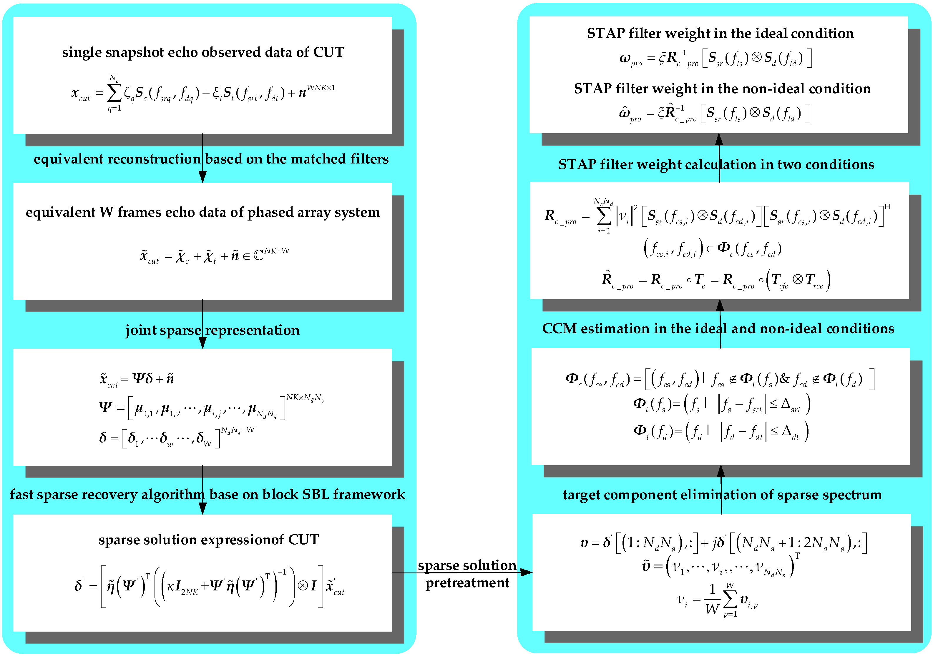
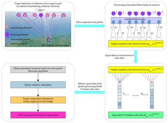
In order to facilitate the understanding of the proposed scheme, its processing flows are clearly shown in Figure 5.
Figure 5 shows that the whole scheme is divided into eight main steps:
(1)
The single snapshot echo observed data of CUT are obtained;
(2)
The equivalent W frames’ echo data of the phased array system can be reconstructed;
(3)
W frames’ echo data are represented by the joint sparse recovery method;
(4)
A fast sparse recovery algorithm based on the block SBL framework is used to obtain the sparse solution expression of the multi-frame echo data of CUT;
(5)
The sparse solution should be previously treated so as to adequately utilize the sparse results of W frames’ echo data;
(6)
The target components in the sparse solution are eliminated based on the approximate prior knowledge;
(7)
CCM can be separately estimated in the ideal and non-ideal conditions;
(8)
The filter weight is calculated to realize clutter suppression in the two conditions.
Combined with the above steps, a corresponding example is given to analyze the proposed scheme. Suppose that N , K , and W are respectively equal to 2, 2, and 2; the single echo observed data can then be expressed as x c u t = x 1 , 1 , 1 , x 2 , 1 , 1 , x 1 , 2 , 1 , x 2 , 2 , 1 , x 1 , 1 , 2 , x 2 , 1 , 2 , x 1 , 2 , 2 , x 2 , 2 , 2 T . Then, the equivalent W frames’ echo data should be donated as x ˜ c u t = x c u t _ 1 , x c u t _ 2 4 × 2 , x c u t _ 1 = x 1 , 1 , 1 , x 1 , 2 , 1 , x 1 , 1 , 2 , x 1 , 2 , 2 T , and x c u t _ 1 = x 2 , 1 , 1 , x 2 , 2 , 1 , x 2 , 1 , 2 , x 2 , 2 , 2 T . If N d and N s are equal to 4, Ψ = μ 1 , 1 , μ 1 , 2 , μ i , j , , μ 4 , 4 4 × 16 , μ i , j = μ i , j , 1 , 1 , μ i , j , 2 , 1 , μ i , j , 1 , 2 , μ i , j , 2 , 2 T , δ = δ 1 , δ 2 16 × 2 , δ 1 = δ 1 , 1 , 1 , δ 1 , 1 , 2 , , δ 1 , 1 , N s , , δ 1 , N d , N s T , and δ 2 = δ 2 , 1 , 1 , δ 2 , 1 , 2 , , δ 2 , 1 , N s , , δ 2 , N d , N s T . Based on these expressions, the dimensions of δ , υ ˜ , Φ c ( f c s , f c d ) are, respectively, 32 × 2 , 16 × 1 , and 4 × 16 . Furthermore, the dimensions of R c _ p r o , ω p r o , T e , R ^ c _ p r o , ω ^ p r o are, respectively, 4 × 4 , 4 × 1 , 4 × 4 , 4 × 4 , and 4 × 1 .

4. Simulation Experiments and Comparative Analyses

To demonstrate the effectiveness of the proposed method and the clutter suppression performance of the adopted UTSD-TSBL-FP algorithm, numerous simulation experiments and comparative analyses are presented in this section. Based on the uniform transmitting subarray diversity with airborne active array, the clutter suppression performance is compared among different sparse recovery algorithms.
Simulation experiments are divided into three main parts: (1) Seven different kinds of sparse recovery algorithm based on the UTSD system are analyzed from the perspectives of the sparse spectrum, improved factor (IF), and running time. These algorithms are orthogonal matching pursuit (OMP), focal underdetermined system solver (FOCUSS), SBL, block sparse Bayesian learning based on bound optimization (BSBL-BO), block sparse Bayesian learning based on expectation-maximization (BSBL-EM), temporally sparse Bayesian learning (TSBL) [40,42,43,47,48,49], and the adopted TSBL-FP. (2) The clutter suppression performance of some different radar systems is compared. (3) To verify the robustness of the algorithms, the STAP performance under different non-ideal conditions is analyzed using the UTSD-TSBL and UTSD-TSBL-FP algorithms. The number of Monte Carlo iterations is 50. The other parameter settings required for the experiments are shown in Table 1.

4.1. STAP Performance Comparison Using Different Algorithms

4.1.1. Simulation Results on the Sparse Spectrum

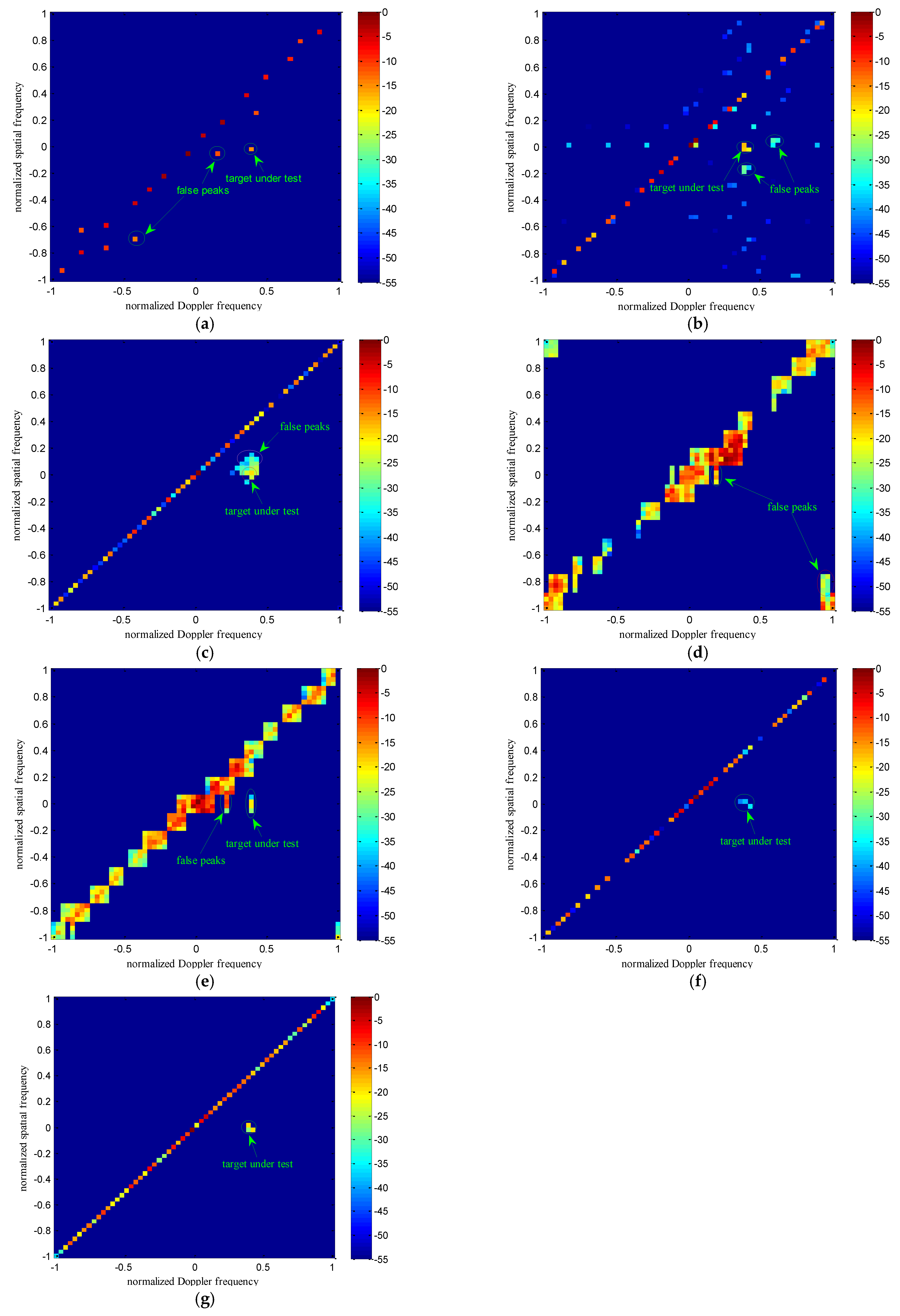
In Figure 6, the sparse spectra of seven sparse recovery algorithms are shown based on the UTSD system. It can be seen that the position of the clutter ridge is generally recovered. However, the phenomenon of incomplete data recovery on the clutter ridge is shown in Figure 6a–f, and the phenomenon of partial false peaks in the sparse spectrum is also presented in Figure 6a–e. These phenomena result in a significant decline in the clutter suppression performance. Moreover, the clutter ridge is evidently broadened in Figure 6d,e, which may further weaken the system capability. Compared with the sparse recovery results of the previous six algorithms, the above three phenomena can be effectively eliminated using the proposed UTSD-TSBL-FP algorithm. Furthermore, according to the quality of the sparse spectrum, the ranking of the seven algorithms, in descending order, is UTSD-TSBL-FP, UTSD-TSBL, UTSD-SBL, UTSD-FOCUSS, UTSD-BSBL-EM, UTSD-BSBL-BO, and UTSD-OMP. Among the seven algorithms, the proposed UTSD-TSBL-FP algorithm has superior sparse recovery performance. Therefore, the false peaks are effectively removed and the defects of clutter data are completely avoided. Finally, the accuracy of CCM estimation can be promoted, which is beneficial to the better suppression of nonhomogeneous clutter and improvement in target detection performance.

4.1.2. Simulation Results on Improved Factor

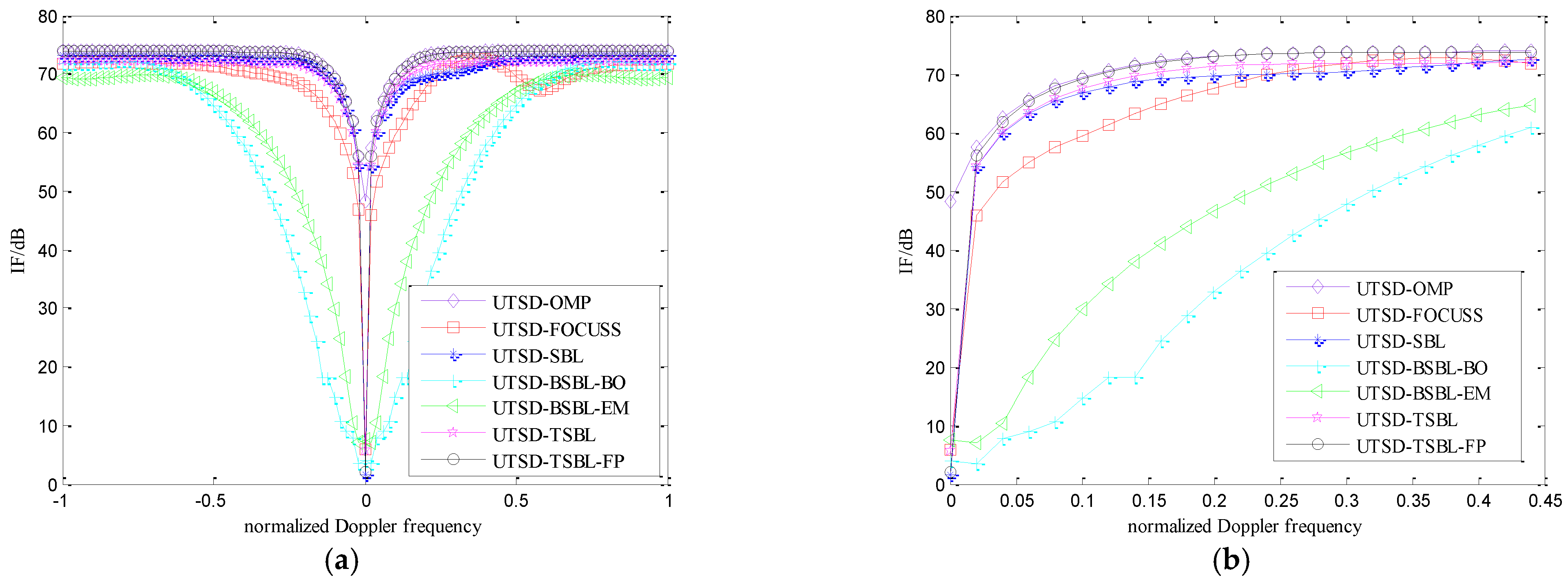
In Figure 7, the clutter suppression performance of these algorithms with UTSD is compared from the perspective of the improved factor (IF), which is one of the key indicators to measure the performance of STAP filters. In general, IF is used to evaluate the effectiveness of the STAP processor. It can be defined as the ratio of the output signal-to-clutter-plus-noise (SCNROUT) to the input signal-to-clutter-plus-noise (SCNRIN). The depth and width of the improved factor gap directly reflect the clutter suppression ability. The deeper and narrower the gap, the better the STAP performance.
Since the accuracy of CCM estimation and clutter filtering weights are restricted to the recovery result of the sparse spectrum, SCNROUT is further impacted and IF is also changed. Figure 7 shows that the clutter suppression performance of the proposed UTSD-TSBL-FP algorithm is obviously better than that of the other six algorithms; this result is closely related to its superior sparse recovery capability. Combined with the depth and width of the IF gap, the ranking of the seven algorithms in descending order of clutter suppression performance is UTSD-TSBL-FP, UTSD-TSBL, UTSD-SBL, UTSD-FOCUSS, UTSD-BSBL-EM, UTSD-BSBL-BO, and UTSD-OMP. For example, with UTSD-BSBL-EM, the depth and width of the IF gap are, respectively, about 62 dB and 1.4. Nevertheless, with the proposed UTSD-TSBL-FP algorithm, the depth and width of the IF gap are, respectively, about 73.8 dB and 0.5, which demonstrates the superior clutter suppression capability of the proposed algorithm.

4.1.3. Simulation Results on Running Time

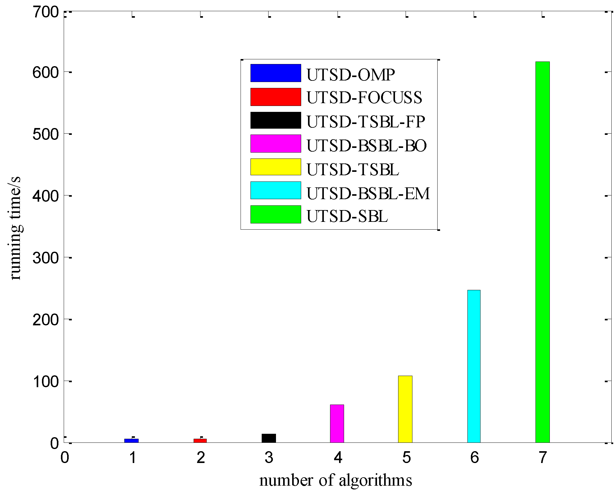
In Figure 8, the running time is shown to reflect the computational burden of different algorithms with the UTSD system. According to the running time, the ranking of these algorithms in descending order is UTSD-SBL, UTSD-BSBL-EM, UTSD-TSBL, UTSD-BSBL-BO, UTSD-TSBL-FP, UTSD-FOCUSS, and UTSD-OMP. In terms of the computational complexity, compared with the other algorithms, the proposed UTSD-TSBL-FP algorithm generally has a certain advantage. Moreover, the proposed algorithm has the shortest running time while simultaneously maintaining the superior clutter suppression performance.
In order to further analyze the computational burden, a kind of theoretical method was used. As for the whole processing scheme, it can be divided into four main parts, namely, single snapshot echo observed data acquisition, equivalent reconstruction of echo data, sparse solution calculation, and clutter suppression. Therefore, the computational load of the scheme is influenced by these four parts. However, in terms of these seven algorithms, the difference in computational burden mainly depends on the third part, and the computational load of the other three parts of each algorithm is similar. The complexity of data acquisition, data reconstruction, and clutter suppression are, respectively, O W N K , O W N K , O N d N s + N 3 K 3 . As for the sparse solution calculation, the computational complexity of the different algorithms can be analyzed using Figure 9.
The relation between the number of iterations and sparse solution complexity is shown in Figure 9. It can be seen that the sparse solution complexity decreases gradually with the increase in iterations. When the number of iterations reaches 300, the sparse solution complexity tends to be low. Thus, the complexity of sparse solution calculation can be expressed as the sum of calculations corresponding to different iterations. If P c , g i are the total number of iterations and the sparse solution complexity of each iteration, respectively, the sparse solution complexity of each algorithm can be approximately denoted as O i = 1 P c g i . Combined with Figure 9, it can be easily verified that the proposed scheme has the lowest computational complexity. Furthermore, the result in Figure 9 is consistent with the running time ranking of the different algorithms shown in Figure 8.
Based on the comprehensive consideration of the sparse spectrum, clutter suppression, and running time, the proposed algorithm has more advantages than the others.

4.2. STAP Performance Comparison Using Different Radar Systems

In this section, the STAP performance is compared of three radar systems, namely, PA radar using the direct data domain (DDD) method [26], multiple-input multiple-output (MIMO) radar [50,51], and airborne active array (AAA) radar using the UTSD method.
Regarding PA radar, the key idea of the DDD method is that CUT can be processed by a sliding window so as to obtain more samples and realize CCM estimation. Its sub-aperture width and sub-pulse size are 4 and 8, respectively. In MIMO radar, four-frame data and sixteen-frame data are separately used to realize the joint sparse processing. In addition, the equivalent multi-frame TSBL-FP algorithm is adopted in both MIMO and AAA-UTSD radar. The other simulation parameter settings are consistent with those shown in Table 1. Specific simulation results are shown in Figure 10 and Figure 11.

4.2.1. Simulation Results on Improved Factor

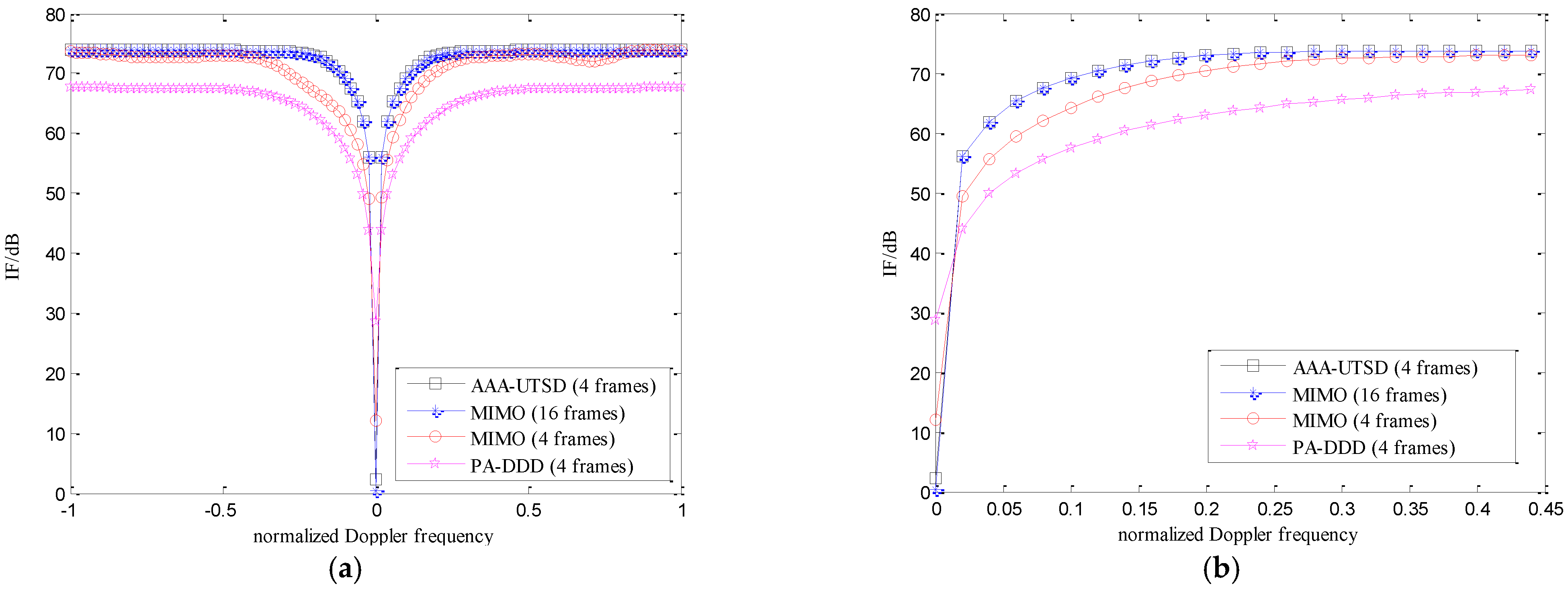
In Figure 10, the STAP performance based on different radar systems is analyzed from the perspective of IF. It can be seen that the ranking of these four cases in descending order is MIMO (sixteen frames), AAA-UTSD (four frames), MIMO (four frames), and PA-DDD (four frames). Concerning MIMO radar, the echo observed data of CUT are also reconstructed with the matching filters. Then, the equivalent sixteen-frame echo data can be obtained. When only equivalent four-frame echo data gained by MIMO radar are selected, its performance is obviously inferior to that of AAA-UTSD radar using the equivalent four-frame echo data. With the four-frame echo data of MIMO radar, the depth and width of the IF gap are about 61 dB and 0.9, respectively. Moreover, there are some fluctuations and a small notch appears in the IF diagram when the normalized Doppler frequency is between 0.6 and 0.8. However, with the four-frame echo data of AAA-UTSD radar, the depth and width of the IF gap are about 73.8 dB and 0.5, respectively. There is no small notch in its diagram. The main reason for this is that the number of data frames used by MIMO radar is not enough, which leads to the inaccurate estimation of CCM and decline in STAP performance. Although the number of data frames is the same in MIMO and AAA-UTSD radar, the directional gain and the coherence processing gain inside the transmitting subarray can be effectively utilized so as to improve the clutter suppression performance of the AAA-UTSD radar.
Furthermore, as the number of data frames increases in MIMO radar, the clutter suppression capability is evidently enhanced. The STAP performance of MIMO radar with sixteen-frame echo data is approximately similar to that of AAA-UTSD radar with the equivalent four-frame echo data. In terms of PA-DDD radar, the four-frame echo data can be obtained using the sliding window method, which cannot effectively avoid the loss of radar aperture and STAP performance.

4.2.2. Simulation Results on Running Time

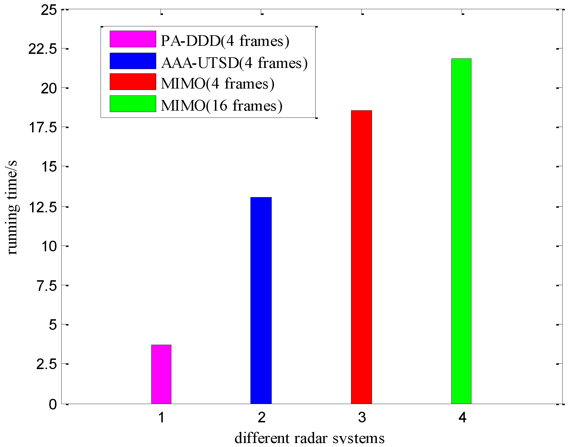
In Figure 11, the running time of different radar systems is shown. It shows that the ranking of these four cases in descending order is MIMO (sixteen frames), MIMO (four frames), AAA-UTSD (four frames), and PA-DDD (four frames). In MIMO radar with sixteen-frame echo data, the computational burden is heavy since the number of data frames increases. Compared with MIMO radar, the running velocity of AAA-UTSD radar with four-frame echo data is higher. The main reason for this is that the dimensions of single snapshot echo observed data of CUT are reduced from M N K × 1 to W N K × 1 when the uniform transmitting subarray diversity (UTSD) method is used in the airborne active array (AAA). Then, combined with the matched reconstruction, the number of equivalent data frames is W and the dimension of single frame data is N K × 1 . Finally, only the equivalent W frames’ echo data are processed by the joint sparse recovery and the running time is significantly reduced. Although the four-frame echo data are also selected in MIMO radar, its running time is still slightly longer than that of AAA-UTSD radar, because the data dimensions of the equivalent reconstruction processing with the former are M N K × 1 .
The computational burden comparison between different radar systems can be also demonstrated in the theoretical view. In the DDD method used in the phased array system, its processing scheme is mainly divided into two parts since data reconstruction and sparse solution are not required. If the sub-aperture width and the sub-pulse size are N m , K m , respectively, the complexity of data acquisition and clutter suppression are respectively expressed as O N K , O N m 3 K m 3 + N m 3 K m 2 N m 1 . In terms of the other two radar systems, the complexity of clutter suppression is the same. However, the complexity of data acquisition, data reconstruction, and sparse solution calculation are different. Regardless of whether MIMO radar uses sixteen-frame echo data or four-frame echo data, the complexity of data acquisition and data reconstruction are O M N K . As for the sparse solution calculation, the computational complexity of different systems can be analyzed using Figure 12.
Figure 12 shows that the sparse solution complexity decreases gradually with the increase in iterations. When the number of iterations reaches 10, the sparse solution complexity tends to be low. In each iteration, the sparse solution complexity of the AAA-UTSD radar system is generally smaller than that of the other systems. Combined with Figure 12, it can be easily verified that the proposed scheme has the lowest computational complexity. Furthermore, the result in Figure 12 is consistent with the running time ranking of different algorithms shown in Figure 11.
These three diagrams show that AAA-UTSD radar has more advantages than MIMO and PA radar in terms of clutter suppression. The proposed method effectively solves the problem of insufficient IID samples. The clutter spectrum is precisely estimated by the joint sparse recovery of the equivalent multi-frame echo data, and the accuracy of CCM estimation is ensured. Moreover, under the premise of ensuring better clutter suppression performance, the computational burden is obviously reduced with the proposed method.

4.3. STAP Performance Comparison in Different Non-Ideal Conditions

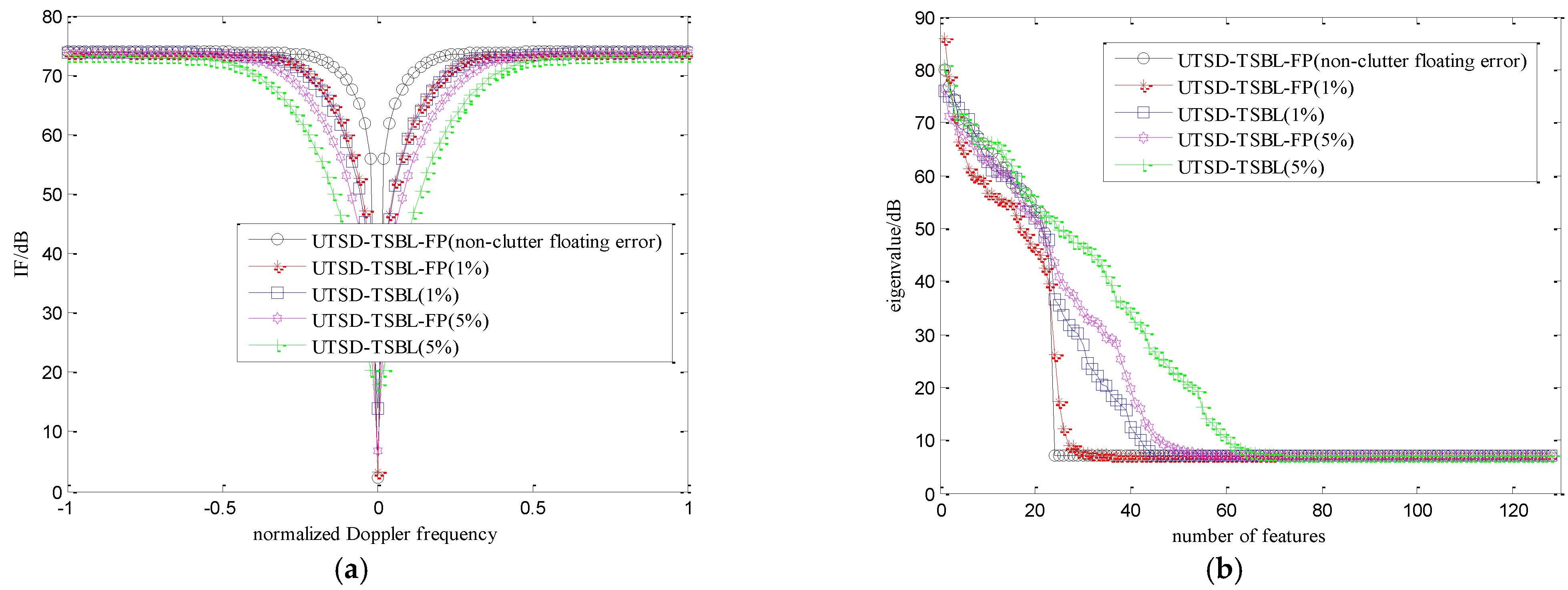
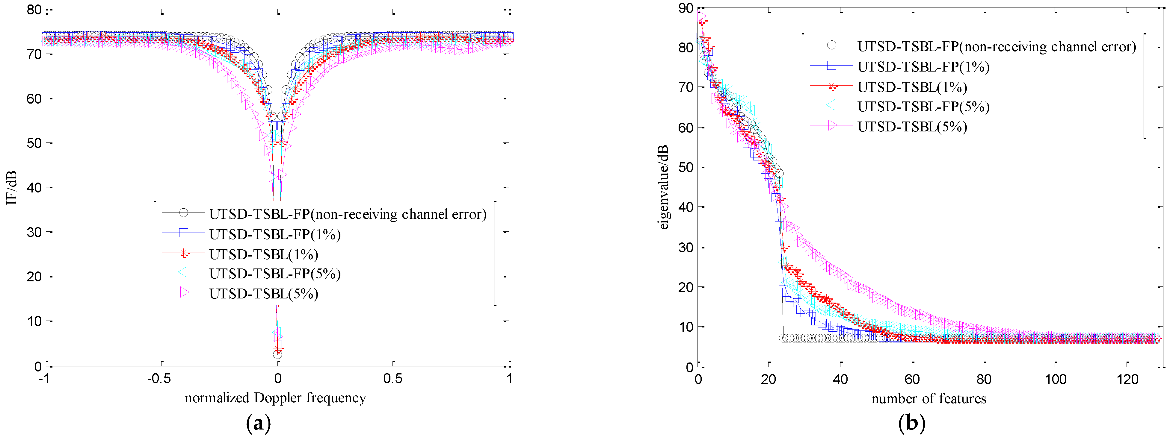
In view of the non-ideal conditions of the real environment, the influence of clutter floating error and receiving channel error on STAP performance should be analyzed. Based on UTSD-TSBL and UTSD-TSBL-FP algorithms, the simulation results of STAP performance in terms of the different non-ideal errors are given in Figure 13 and Figure 14.
The influence of STAP performance on clutter floating error and receiving channel error are shown in Figure 13 and Figure 14, respectively. Combined with the performance comparison results, the figures show that when the non-ideal errors are considered, the performance of the proposed UTSD-TSBL-FP algorithm declines to a certain extent. However, under the same error condition, the algorithm’s performance is significantly better than that of UTSD-TSBL algorithm. The main reason for this is that the existence of non-ideal factors changes the original clutter internal structure and local correlation, which leads to the deviation in the STAP adaptive filtering weights and the decrease in SCNROUT. Compared with the UTSD-TSBL algorithm, not only can the clutter sparse spectrum be recovered better, but the defects of data on the clutter ridge and the emergence of false peaks can also be avoided by the proposed method. Moreover, both the accuracy of CCM estimation and STAP performance with non-ideal errors are obviously improved.
With the increase in error, the number of large eigenvalues in the clutter data increases. Its influence on the UTSD-TSBL algorithm is more obvious. This is because the increase in the error weakens the correlation among the internal clutter patches and increases the number of independent clutter blocks. Furthermore, due to the data dropout of the clutter spectrum recovered by the UTSD-TSBL algorithm, CCM estimation is inaccurate. The interaction of these two reasons further reduces the algorithm’s STAP performance. However, the number of large eigenvalues with the proposed UTSD-TSBL-FP algorithm can result in relatively slower growth under the same error conditions, and has a certain relation with the quality of the clutter sparse recovery. Therefore, the robustness of the proposed algorithm is superior.

5. Conclusions

Nonhomogeneous ground clutter suppression is crucial when low-altitude targets are detected by airborne radar. In consideration of the apparent spatial–temporal coupling property of ground clutter, the space–time adaptive processing technique is widely applied to realize clutter suppression. However, the majority of the current methods were proposed to address the problem that the number of IID training samples is not sufficient. Although the demanded IID sample size is evidently reduced by many of these improved approaches, the processing performance of airborne system is also influenced. Furthermore, with the further deterioration in the heterogeneous clutter environment, IID samples may be extremely deficient, and various schemes used to suppress the ground clutter may be invalid. Moreover, considering that the active array radar has many unique advantages, such as multiple transceiver configurations, transmission of waveform diversity, and flexible spatial selectivity, its application can provide more opportunities for clutter suppression.
Therefore, to address the above problem, in this paper, a novel robust space–time joint sparse processing method is proposed based on the uniform transmitting subarray diversity of the airborne active array. The proposed scheme can only adopt the single snapshot CUT data to efficiently accomplish clutter suppression, and does not regard the quantity and quality of the training samples. The specific treatment processes of this method are divided into three steps. First, the signal model of uniform transmitting subarray diversity is established to obtain the single snapshot echo observed data. Second, with the matched reconstruction in the receiver, the single snapshot data can be equivalently transformed into multi-frame echo data of the phased array system. Third, considering that there is high similarity among the equivalent multi-frame echo data, the block sparsity is satisfied and multi-frame echo data joint sparse recovery can be applied. Therefore, a fast equivalent multi-frame echo data joint sparse processing algorithm based on SBL is adopted to obtain the clutter sparse spectrum and calculate the adaptive filtering weight of STAP. Finally, based on the results of numerous experiments, the clutter suppression performance, computational burden, and robustness of the proposed method are compared with those of other schemes. This comparison demonstrates that the proposed approach can reduce the computational complexity while maintaining better clutter suppression performance. In particular, the proposed approach successfully overcomes the limitation of the number and quality of IID training samples on STAP processing, It also effectively avoids the deterioration in the clutter suppression performance due to the extreme deficiency of IID training samples in a severely nonhomogeneous environment.

Author Contributions

Q.W. and X.H. proposed the signal model and clutter suppression method; B.X., G.W. and W.Z. constructed and designed the simulation experiments; Q.W. and B.X. completed the paper writing; G.W. and W.Z. put the finishing touches to this paper. All authors have read and agreed to the published version of the manuscript.

Funding

This research was funded by the National Natural Science Foundation of China under Grants 62001479 (Q.W.), 62106277 (B.X.), by the School Scientific Research Program of National University of Defense Technology under Grants ZK19-28 (Q.W.), ZK21-39 (B.X.), by the Information and Communication Business Cost Project of JSCMC under Grant ZLKT-XT-2147(B.X., Q.W.).

Conflicts of Interest

The authors declare no conflict of interest.

References

  1. Barbarossa, S.; Picardi, G. Predictive Adaptive Moving Target Indicator. Signal Process. 1986, 10, 83–97. [Google Scholar] [CrossRef]
  2. Chen, B.X. Modern Radar System Analysis and Design; Xidian University Press: Xi’an, China, 2012. [Google Scholar]
  3. Liu, Z.; Ho, D.K.C; Xu, X.Q.; Yang, J.Y. Moving Target Indication Using Deep Convolutional Neural Network. IEEE Access 2018, 6, 65651–65660. [Google Scholar] [CrossRef]
  4. Wang, Y.L.; Peng, Y.N. Space-Time Adaptive Processing; Tsinghua University Press: Beijing, China, 2000. [Google Scholar]
  5. Brennan, L.E.; Mallett, J.D.; Reed, I.S. Theory of Adaptive Radar. IEEE Trans. Aerosp. Electron. Syst. 1973, 9, 237–251. [Google Scholar] [CrossRef]
  6. Jia, F.D.; Sun, G.H.; He, Z.S.; Li, J. Grating-Lobe Clutter Suppression in Uniform Subarray for Airborne Radar STAP. IEEE Sens. J. 2019, 19, 6956–6965. [Google Scholar] [CrossRef]
  7. Reed, I.S.; Mallett, J.D.; Brennan, L.E. Rapid Convergence Rate in Adaptive Arrays. IEEE Trans. Aerosp. Electron. Syst. 1974, 10, 853–863. [Google Scholar] [CrossRef]
  8. Shi, J.X; Xie, L.; Cheng, Z.Y.; He, Z.S.; Zhang, W. Angle-Doppler Channel Selection Method for Reduced-Dimension STAP Based on Sequential Convex Programming. IEEE Commun. Lett. 2021, 25, 3080–3084. [Google Scholar] [CrossRef]
  9. Sui, J.X.; Wang, J.; Zuo, L.; Gao, J. Cascaded Least Square Algorithm for Strong Clutter Removal in Airborne Passive Radar. IEEE Trans. Aerosp. Electron. Syst. 2022, 58, 679–696. [Google Scholar] [CrossRef]
  10. Chen, N.K.; Wei, P.; Ai, X.Y. A Robust STAP Method Based on Alternating Projection and Clutter Cancellation. IEEE Access 2017, 7, 179880–179890. [Google Scholar] [CrossRef]
  11. Yang, Z.C.; Wang, X.Y. Reduced-Rank Space-Time Adaptive Processing Algorithm Based on Multistage Selections of Angle-Doppler Filters. IET Radar Sonar Navig. 2022, 16, 327–345. [Google Scholar] [CrossRef]
  12. Cao, C.H.; Zhang, J.; Meng, J.M.; Zhang, X.; Mao, X.P. Clutter Suppression and Target Tracking by the Low-Rank Representation for Airborne Maritime Surveillance Radar. IEEE Access 2020, 8, 160774–160789. [Google Scholar] [CrossRef]
  13. Huang, P.H.; Zou, Z.H.; Xia, X.G.; Liu, X.Z.; Liao, G.S. A Novel Dimension-Reduced Space-Time Adaptive Processing Algorithm for Spaceborne Multichannel Surveillance Radar Systems Based on Spatial-Temporal 2-D Sliding Window. IEEE Trans. Geosci. Remote Sens. 2022, 60, 5109721. [Google Scholar] [CrossRef]
  14. Wang, X.Y.; Yang, Z.C.; Huang, J.J.; Lamare, R.C.D. Robust Two-Stage Reduced-Dimension Sparsity-Aware STAP for Airborne Radar with Coprime Arrays. IEEE Trans. Signal Process. 2020, 68, 81–96. [Google Scholar] [CrossRef]
  15. Shi, B.; Hao, C.P.; Hou, C.H.; Ma, X.C.; Peng, C.Y. Parametric Rao Test for Multichannel Adaptive Detection of Range-Spread Target in Partially Homogeneous Environments. Signal Process. 2015, 108, 421–429. [Google Scholar] [CrossRef]
  16. Jiang, C.S.; Li, H.B.; Rangaswamy, M. Conjugate Gradient Parametric Detection of Multichannel Signals. IEEE Trans. Aerosp. Electron. Syst. 2012, 48, 1521–1536. [Google Scholar] [CrossRef]
  17. Zhao, Y.; Wan, S.H.; Lu, S.T.; Sun, J.P.; Lei, P. Exploiting the Persymmetric Property of Covariance Matrices for Knowledge-Aided Space-Time Adaptive Processing. IEEE Access 2018, 6, 68001–68012. [Google Scholar] [CrossRef]
  18. Sun, G.H.; He, Z.S.; Tong, J.; Zhang, X.J. Knowledge-Aided Covariance Matrix Estimation via Kronecker Product Expansions for Airborne STAP. IEEE Geosci. Remote Sens. Lett. 2018, 15, 527–531. [Google Scholar] [CrossRef]
  19. Zhang, W.; He, Z.S.; Li, H.Y. Space Time Adaptive Processing Based on Sparse Recovery and Clutter Reconstructing. IET Radar Sonar Navig. 2019, 13, 789–794. [Google Scholar] [CrossRef]
  20. Hu, J.F.; Xia, Y.Y.; Li, H.Y.; Liang, J.; Lin, T. A Joint Sparse Space-time Adaptive Processing Method. IEEE Access. 2016, 4, 1–7. [Google Scholar] [CrossRef]
  21. Liu, M.X.; Zou, L.; Yu, X.L.; Zhou, Y.; Wang, X.G.; Tang, B. Knowledge Aided Covariance Matrix Estimation via Gaussian Kernel Function for Airborne SR-STAP. IEEE Access 2020, 8, 5970–5978. [Google Scholar] [CrossRef]
  22. Guo, L.; Deng, W.B.; Yao, D.; Yang, Q.; Ye, L.; Zhang, X. A Knowledge-Based on Auxiliary Channel STAP for Target Detection in Shipborne HFSWR. Remote Sens. 2021, 13, 621. [Google Scholar] [CrossRef]
  23. Liu, K.; Wang, T.; Wu, J.X.; Chen, J.M. A Two-Stage STAP Method Based on Fine Doppler Localization and Sparse Bayesian Learning in the Presence of Arbitrary Array Errors. Sensors 2022, 22, 77. [Google Scholar] [CrossRef] [PubMed]
  24. Cui, N.; Xing, K.; Duan, K.Q.; Yu, Z.J. Knowledge-Aided Block Sparse Bayesian Learning STAP for Phased-Array MIMO Airborne Radar. IET Radar Sonar Navig. 2021, 15, 1628–1642. [Google Scholar] [CrossRef]
  25. Cristallini, D.; Bürger, W. A Robust Direct Data Domain Approach for STAP. IEEE Trans. Signal Process. 2012, 60, 1283–1294. [Google Scholar] [CrossRef]
  26. Yang, Z.C.; Fa, R.; Qin, Y.L.; Li, X.; Wang, H.Q. Direct Data Domain Sparsity-Based STAP Utilizing Subaperture Smoothing Techniques. Int. J. Antenna Propag. 2015, 2015, 171808. [Google Scholar] [CrossRef] [Green Version]
  27. Li, M.; Sun, G.H.; He, Z.S. Direct Data Domain STAP Based on Atomic Norm Minimization. In Proceedings of the 2019 IEEE Radar Conference, Boston, MA, USA, 22–26 April 2019; pp. 1–6. [Google Scholar]
  28. Gao, Z.Q.; Tao, H.H. Knowledge-Aided Direct Data Domain STAP Algorithm for Forward-looking Airborne Radar. In Proceedings of the 2019 IEEE International Conference on Signal, Information and Data Processing (ICSIDP), Chongqing, China, 11–13 December 2019; pp. 1–6. [Google Scholar]
  29. Xiao, H.; Wang, T.; Wen, C.; Ren, B. A Generalized Eigenvalue Reweighting Covariance Matrix Estimation Algorithm for Airborne STAP Radar in Complex Environment. IET Radar Sonar Navig. 2021, 15, 1309–1324. [Google Scholar] [CrossRef]
  30. Bil, R.; Holpp, W. Modern Phased Array Radar Systems in Germany. In Proceedings of the 2016 IEEE International Symposium on Phased Array Systems and Technology (PAST), Waltham, MA, USA, 18–21 October 2016; pp. 1–7. [Google Scholar]
  31. Alkhafaji, N.; Campbell, R.L.; Roche, M. Microwave Modulated Scatter Active Array Distortion Sidelobes. IEEE Trans. Microw. Theory Tech. 2020, 68, 328–338. [Google Scholar] [CrossRef]
  32. Kinghorn, T.; Scott, I.; Totten, E. Recent Advances in Airborne Phased Array Radar Systems. In Proceedings of the 2016 IEEE International Symposium on Phased Array Systems and Technology (PAST), Waltham, MA, USA, 18–21 October 2016; pp. 1–7. [Google Scholar]
  33. Burger, W.K. Sidelobe Forming for Ground Clutter and Jammer Suppression for Airborne Active Array Radar. In Proceedings of the IEEE International Symposium on Phased Array Systems and Technology, Boston, MA, USA, 14–17 October 2003; pp. 271–276. [Google Scholar]
  34. Rose, P.S.; Finlay, C.D. Reducing Clutter in Airborne Radars Equipped with Active Electronically Steered Array Antennas by Using a Novel Receive Aperture Weighting. In Proceedings of the 2008 IEEE Radar Conference, Rome, Italy, 26–30 May 2008; pp. 573–577. [Google Scholar]
  35. Wijenayake, C.; Madanayake, A.; Belostotski, L.; Xu, Y.; Bruton, L. All-Pass Filter-Based 2-D IIR Filter-Enhanced Beamformers for AESA Receivers. IEEE Trans. Circuits Syst. I-Regul. Pap. 2014, 61, 1331–1342. [Google Scholar] [CrossRef]
  36. Buerger, W.; Perna, I. Knowledge Aided STAP/GMTI with Subarrayed AESA Radar. In Proceedings of the EUSAR 2016: 11th European Conference on Synthetic Aperture Radar (EUSAR), Hamburg, Germany, 7–9 June 2016; pp. 220–225. [Google Scholar]
  37. Zhang, X.C.; Xie, W.C.; Zhang, Y.S.; Wang, Y.L. Modeling and Analysis of the Clutter on Airborne MIMO Radar with Arbitrary Waveform Correlation. J. Electron. Inf. Technol. 2011, 33, 646–651. [Google Scholar] [CrossRef]
  38. Zhang, X.C.; Zhang, Y.S.; Xie, W.C.; Wang, Y.L. Research on the Estimation of Clutter Rank for Coherent Airborne MIMO Radar. J. Electron. Inf. Technol. 2011, 33, 2125–2131. [Google Scholar] [CrossRef]
  39. Feng, W.K.; Zhang, Y.S. MMV-JSR Based STAP Method Using MIMO Radar. IEICE Comm. Express. 2016, 5, 163–168. [Google Scholar] [CrossRef] [Green Version]
  40. Gan, F.P.; Wang, H.B.; Fang, Y.; Zhang, K.; Qin, G.-J.; Zhao, X. Reconstruction of Heart Sound Based on CS and BSBL. Comput. Eng. Des. 2016, 37, 1037–1041. [Google Scholar]
  41. Jiang, K.; Wang, H.F.; Shahidehpour, M.; He, B.T. Block-Sparse Bayesian Learning Method for Fault Location in Active Distribution Networks with Limited Synchronized Measurements. IEEE Trans. Power Syst. 2021, 36, 3189–3203. [Google Scholar] [CrossRef]
  42. Zhang, Z.L.; Rao, B.D. Sparse Signal Recovery with Temporally Correlated Source Vectors Using Sparse Bayesian Learning. IEEE J. Sel. Top. Signal Process. 2011, 5, 912–926. [Google Scholar] [CrossRef] [Green Version]
  43. Song, Q.J. Research on Sparse Bayesian Learning Base Sparse Channel Estimation in Underwater Acoustic OFDM Communication. Ph.D. Thesis, Harbin Engineering University, Harbin, China, 2020. [Google Scholar]
  44. Qiao, G.; Song, Q.J.; Ma, L.; Liu, S.Z.; Sun, Z.; Gan, S. Sparse Bayesian Learning for Channel Estimation in Time-Varying Underwater Acoustic OFDM Communication. IEEE Access 2018, 6, 56675–56684. [Google Scholar] [CrossRef]
  45. Zhang, Z.L.; Rao, B.D. Recovery of Block Sparse Signals Using the Framework of Block Sparse Bayesian Learning. In Proceedings of the 2012 IEEE International Conference on Acoustics, Speech and Signal Processing (ICASSP), Kyoto, Japan, 25–30 March 2012; pp. 3345–3348. [Google Scholar]
  46. MacKay, D.J.C. Bayesian Interpolation. Neural Comput. 1992, 4, 131–134. [Google Scholar] [CrossRef]
  47. Tropp, J.A.; Gilbert, A.C. Signal Recovery from Random Measurements via Orthogonal Matching Pursuit. IEEE Trans. Info. Theory 2007, 53, 4655–4666. [Google Scholar] [CrossRef] [Green Version]
  48. Gorodnitsky, I.F.; Rao, B.D. Sparse Signal Reconstruction from Limited Data Using FOCUSS: A Re-Weighted Minimum Norm Algorithm. IEEE Trans. Signal Process. 1997, 45, 600–616. [Google Scholar] [CrossRef] [Green Version]
  49. Balkan, O.; Kreutz-Delgado, K.; Makeig, S. Localization of More Sources than Sensors via Jointly Sparse Bayesian Learning. IEEE Signal Process. 2014, 21, 131–134. [Google Scholar] [CrossRef]
  50. Shi, J.P.; Yang, Z.; Liu, Y.X. On Parameter Identifiability of Diversity-Smoothing-Based MIMO Radar. IEEE Trans. Aerosp. Electron. Syst. 2021, in press. [CrossRef]
  51. Wang, X.P.; Yang, L.T.; Dong, M.X.; Ota, K.; Wang, H.F. Multi-UAV Cooperative Localization for Marine Targets Based on Weighted Subspace Fitting in SAGIN Environment. IEEE Internet Things J. 2022, 9, 5708–5718. [Google Scholar] [CrossRef]
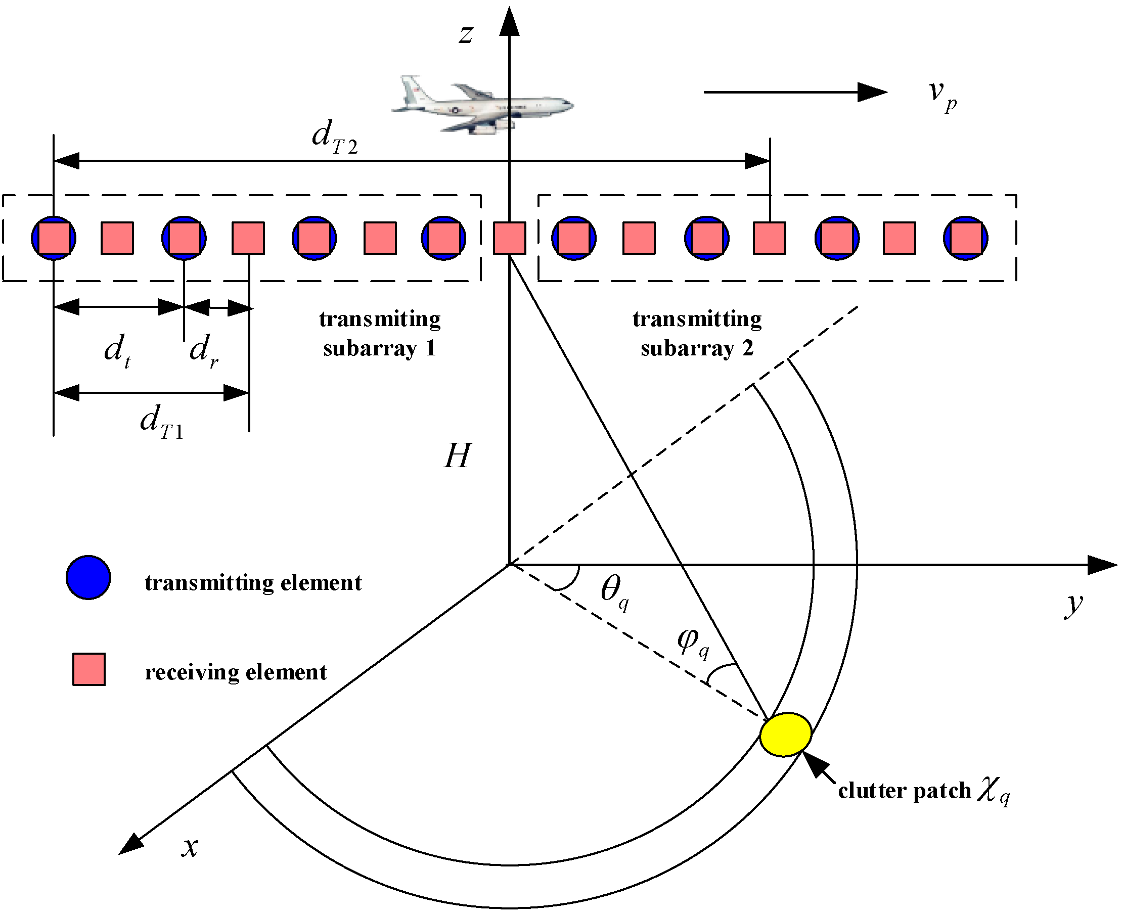
Figure 1. Spatial geometric relation of the airborne active side-looking array based on the transmitting subarray diversity.
Remotesensing 14 02647 g001
Figure 2. Spatial structure of the transmitting subarray.
Remotesensing 14 02647 g002
Figure 3. Schematic diagram of acquiring the echo data by the airborne active array radar with transmitting subarray diversity.
Remotesensing 14 02647 g003
Figure 4. Schematic diagram for obtaining multi-frame echo data with equivalent reconstruction.
Remotesensing 14 02647 g004
Figure 5. Flowchart of the proposed robust space-time joint sparse processing scheme.
Remotesensing 14 02647 g005
Figure 6. Sparse spectrum comparison of different algorithms: (a) sparse spectrum with UTSD-OMP; (b) sparse spectrum with UTSD-FOCUSS; (c) sparse spectrum with UTSD-SBL; (d) sparse spectrum with UTSD-BSBL-BO; (e) sparse spectrum with UTSD-BSBL-EM; (f) sparse spectrum with UTSD-TSBL; (g) sparse spectrum with UTSD-TSBL-FP.
Remotesensing 14 02647 g006
Figure 7. Improved factor comparison of different algorithms with UTSD: (a) improved factor performance; (b) local improved factor performance.
Remotesensing 14 02647 g007
Figure 8. Running time comparison of different algorithms with UTSD.
Remotesensing 14 02647 g008
Figure 9. Running time comparison of different algorithms with UTSD.
Remotesensing 14 02647 g009
Figure 10. Improved factor comparison of different radar systems: (a) improved factor comparison; (b) local improved factor comparison.
Remotesensing 14 02647 g010
Figure 11. Running time comparison of different radar systems.
Remotesensing 14 02647 g011
Figure 12. Computational complexity comparison of sparse solution calculation.
Remotesensing 14 02647 g012
Figure 13. Performance comparison of two algorithms with clutter floating error: (a) improved factor; (b) clutter eigenvalue spectrum.
Remotesensing 14 02647 g013
Figure 14. Performance comparison of two algorithms with receiving channel error: (a) improved factor; (b) clutter eigenvalue spectrum.
Remotesensing 14 02647 g014
Table 1. Simulation parameters based on airborne active array.
ParameterValueParameterValue
transmitting element size16number of coherent pulses8
receiving element size16airborne velocity (m/s)140
radar wavelength (m)0.23airborne height (m)8000
number of transmitting subarrays4target velocity (m/s)28
number of elements in each subarray4signal-to-noise ratio (dB)20
transmitting element interval (m)0.115clutter-to-noise ratio (dB)60
receiving element interval (m)0.115normalized temporal frequency0.4
pulse repetition frequency (Hz)2434.8normalized spatial frequency0
Publisher’s Note: MDPI stays neutral with regard to jurisdictional claims in published maps and institutional affiliations.