Extrapolation Assessment for Forest Structural Parameters in Planted Forests of Southern China by UAV-LiDAR Samples and Multispectral Satellite Imagery

Abstract

Accurate estimation and extrapolation of forest structural parameters in planted forests are essential for monitoring forest resources, investigating their ecosystem services (e.g., forest structure and functions), as well as supporting decisions for precision silviculture. Advances in unmanned aerial vehicle (UAV)-borne Light Detection and Ranging (LiDAR) technology have enhanced our ability to precisely characterize the 3-D structure of the forest canopy with high flexibility, usually within forest plots and stands. For wall-to-wall forest structure mapping in broader landscapes, samples (transects) of UAV-LiDAR datasets are a cost-efficient solution as an intermediate layer for extrapolation from field plots to full-coverage multispectral satellite imageries. In this study, an advanced two-stage extrapolation approach was established to estimate and map large area forest structural parameters (i.e., mean DBH, dominant height, volume, and stem density), in synergy with field plots and UAV-LiDAR and GF-6 satellite imagery, in a typical planted forest of southern China. First, estimation models were built and used to extrapolate field plots to UAV-LiDAR transects; then, the maps of UAV-LiDAR transects were extrapolated to the whole study area using the wall-to-wall grid indices that were calculated from GF-6 satellite imagery. By comparing with direct prediction models that were fitted by field plots and GF-6-derived spectral indices, the results indicated that the two-stage extrapolation models (R² = 0.64–0.85, rRMSE = 7.49–26.85%) obtained higher accuracy than direct prediction models (R² = 0.58–0.75, rRMSE = 21.31–38.43%). In addition, the effect of UAV-LiDAR point density and sampling intensity for estimation accuracy was studied by sensitivity analysis as well. The results showed a stable level of accuracy for approximately 10% of point density (34 pts·m⁻²) and 20% of sampling intensity. To understand the error propagation through the extrapolation procedure, a modified U-statistics uncertainty analysis was proposed to characterize pixel-level estimates of uncertainty and the results demonstrated that the uncertainty was 0.75 cm for mean DBH, 1.23 m for dominant height, 14.77 m³·ha⁻¹ for volume and 102.72 n·ha⁻¹ for stem density, respectively.

1. Introduction

As one of the key components of global forest ecosystem, planted forests play a significant role in environmental and economic services, such as mitigating climate change, promoting carbon sequestration, protecting biodiversity, and supplementing wood [1,2,3,4]. Since the 1990s, planted forests’ total area has increased approximately 123 million ha, while natural regenerated forests’ area has declined [5]. In the past decades, significant efforts have been made by China to develop planted forests. Now, China is the country with the largest planted forest area in the world, accounting for 28.4% of the global planted forest resource [6].

In order to implement precision silviculture strategies, it is helpful for forest managers to use advanced digital technologies (e.g., remote sensing) to support site-specific sustainable management decision making and improve silviculture efficiency [7,8]. Benefiting from precision silviculture, planted forests may further increase site productivity or ecological value for economics and society [9,10]. Accurate estimation and extrapolation of forest structural parameters are critical for planted forests to characterize forest composition and structure [11,12]. However, conventional inventory methods based on field measurements have the limitations of being time-consuming and labor-intensive, as well as having the objectivity and consistency challenges of manual measurements [13,14].

In the past few decades, remote sensing techniques have been utilized in forest management practices to provide multi-scale, multi-dimension, and spatially continuous Earth observation data [14,15,16]. Optical satellite images have the advantages of acquiring spectral and textural information, and thus have been widely applied in estimating forest structural parameters, such as stand height [17,18], aboveground biomass (AGB) [19,20], leaf area index [21,22], and canopy cover [23]. Previous studies have indicated that higher resolution remote sensing data help improve estimation accuracy [24,25,26]. The development of very high spatial resolution (VHSR) imagery (e.g., the Chinese Gaofen series data of satellites, GF) has made it possible to enrich observation information and promote inventory practices. The Gaofen series satellites covered a variety of types from panchromatic, multispectral, to hyperspectral, from optics to radar, from solar synchronous orbit to geosynchronous orbit, etc. GF formed an Earth observation system with high spatial resolution. There were several available satellite data about the GF-1 optical satellite with 2 m panchromatic (PAN) and 8/16 m multispectral (MS) bands [27], GF-2 optical satellite with 1 m PAN and 4 m MS bands [28], GF-3 SAR satellite carrying a C-band (~5.3 GHz) SAR sensor with different polarizations [29], GF-4 geostationary-orbit-based Earth observing satellite [30], GF-5 satellite that can simultaneously make comprehensive observations of land and atmosphere [31], and GF-6 optical satellite with 2 m PAN and 8/16 m MS bands [32]. Zhang et al. (2015) [24] used GF-1 satellite imagery-derived spectral and textural indices to improve biomass estimation accuracy for Populus euphratica. Zhou et al. (2020) [33] compared GF-2 satellite imagery with SPOT6 imagery for the estimation of forest structural parameters using machine learning technology. The results indicated that GF-2 results outperformed SPOT6 results. Li et al. (2021) [34] proposed that there is considerable potential to integrate GF-1 and GF-6 imageries with random forest (RF) algorithms to study jujube abandonment.

In contrast to optical remote sensing technologies, Light Detection and Ranging (LiDAR) is an active remote sensing technology and can characterize the three-dimensional (3-D) structure of vegetation [35,36]. LiDAR sensors can measure the distance between emitted and returned laser pulses by penetrating through the forest canopy and generating 3-D point clouds [37]. In recent years, airborne LiDAR has been proven to be a valuable tool in estimating forest structural parameters, e.g., stand height [38], diameter at breast height (DBH) [39], volume [40], stem density [41], and biomass [42]. The most widely applied approach for estimating forest structural parameters is the area-based approach (ABA) which combines LiDAR-derived point cloud metrics with field plots in estimation models [43,44]. It shows the performance of airborne LiDAR to generate wall-to-wall estimates that rely on the coverage of LiDAR data.

However, given the data acquisition and processing cost of airborne LiDAR, it has limited applications in broader landscapes. A cost-effective solution for forest structural parameter estimation in large landscapes is to integrate LiDAR transects (or samples) with optical satellite imagery [45,46]. Wulder et al. (2007) [47] integrated profiling LiDAR transects with Landsat ETM+ imagery and demonstrated improved effects to characterize forest structure over broad areas. Hopkinson et al. (2011) [48] detailed an airborne LiDAR sampling mission of the Canadian boreal forest and suggested the potential of LiDAR transects for spatial extrapolation. Matasci et al. (2018) [46] mapped forest structural parameters over about 552 million ha of the boreal forest of Canada using Landsat composites and representative sampling LiDAR plots.

In recent years, unmanned aerial vehicles (UAVs) have rapidly developed and have successfully been implemented for forestry purposes. Due to the advantages of low cost, flying flexibility, and reliability of data collection [49,50], UAVs have become a promising alternative platform for precision silviculture applications. High spatial and temporal resolution data have been acquired by UAVs at the fine scale [51]. Moreover, UAVs can carry various kinds of sensors to acquire different data. UAVs can perform custom flight missions under user-designed trajectory, mission time, flight speed, and sensor parameters [50]. As UAV payload capacity has increased and LiDAR sensors have become lighter, recent studies have been able to employ multi-rotor UAV-LiDAR systems to collect LiDAR data and estimate forest structural parameters. Wallace et al. (2012) [51] reported an earlier study of UAV-LiDAR in forestry applications. Liu et al. (2018) [52] proved the good performance of UAV-LiDAR for estimating forest structural parameters at the stand level in the Ginkgo plantation. Peng et al. (2020) [53] used several modeling algorithms to assess the capability of UAV-LiDAR data, and the results indicated that Lorey’s height achieved the best estimation accuracy (rRMSE = 10.60–12.05%); additionally, basal area was 15.37–15.87%, AGB was 26.75–37.03%, and stem density was 26.76–27.44%.

Typically, UAV-LiDAR data are acquired over small areas (e.g., samples or transects) rather than wall-to-wall coverage. It may provide a more affordable solution if UAV-LiDAR is used as the bridging data for large area forest structural parameter estimation [54]. In other words, UAV-LiDAR transects can be considered as an intermediate layer of extrapolation to bridge field plots and satellite imagery, due to high estimation accuracy of UAV-LiDAR [45,49,55]. During the extrapolation process, a spatial extrapolation method was proposed [54]. First, UAV-LiDAR-derived metrics were generated to model and map forest structural parameters with field plots. Second, UAV-LiDAR mapping products were then used as reference data to calibrate wall-to-wall satellite imagery. The spatial extrapolation of forest structural parameters from UAV transects or field plots to a large area of interest showed its promising possibility in the extrapolation scheme [46,56]. Wang et al. (2020) [55] employed the spatial extrapolation method to estimate AGB in a mangrove forest. They first generated intermediate AGB products of UAV transects by linking UAV-LiDAR metrics to field plots. Then, full-coverage Sentinel-2 imagery-derived indices in synergy with UAV AGB products were used to estimate AGB in a large area. They found that the AGB estimation result using the spatial extrapolation method acquired higher accuracy (R² = 0.62, RMSE = 50.36 Mg·ha⁻¹) than the conventional method (R² = 0.52, RMSE = 56.63 Mg·ha⁻¹) that directly connected field plots with Sentinel-2 imagery. However, most previous studies have focused on medium or high spatial resolution satellite imagery, for instance, MODIS [57,58], Landsat [59,60], or Sentinel-2 [61], instead of VHSR imagery. Moreover, some studies used the bridging data to undertake spatial extrapolation by airborne [46] or spaceborne LiDAR data [62] that had higher cost or lower resolution than UAV-LiDAR.

For the aspect of lowering data acquisition cost, it is a practical consideration to set a suitable point density while flying UAV-LiDAR. It is worth considering how to balance the point density and estimation accuracy. The sensitivity analysis for the point density decimation is helpful to test the best feasible solution. Furthermore, a suitable point density also helps improve computing efficiency for large area forest structural parameter estimation and mapping.

The key to understanding the quality of forest structural parameter maps is to quantify uncertainty so that error may be propagated from plots to pixels [63]. During the spatial extrapolation procedure, it is vital to assess the error propagation because estimation models are built twice and error is propagated twice in the two-stage workflow. Furthermore, pixel-level estimates of uncertainty maps make it straightforward to show the spatial distribution of error. Chave et al. (2004) [64] analyzed the error propagation into a consistent framework when estimating tropical forest biomass by quantifying four types of uncertainty, including tree measurement, allometric models, sampling uncertainty, and plot representativeness. Chen et al. (2015) [65] assessed the uncertainty of AGB by propagating errors from trees to plots to pixels using airborne LiDAR data, and quantified the uncertainty of AGB at the pixel level.

To the best our knowledge, few researchers have assessed the effectiveness of extrapolation for forest structure estimations in combination with UAV-LiDAR and GF-6 multispectral satellite imagery in planted forests of southern China. In this study, an advanced two-stage extrapolation approach with the capability of uncertainty propagation analysis was established to generate maps of forest structural parameters by coupling field plots, UAV-LiDAR data, and GF-6 imagery. The specific objectives of this study were (1) to estimate and map large area forest structural parameters of a planted forest using UAV-LiDAR transects and GF-6 imagery; (2) to assess the sensitivity of estimation results for UAV-LiDAR data by adjusting point density and sampling intensity; and (3) to evaluate the effectiveness of the advanced two-stage extrapolation approach and determine the uncertainties of pixel-level estimates in the procedure.

2. Materials and Methods

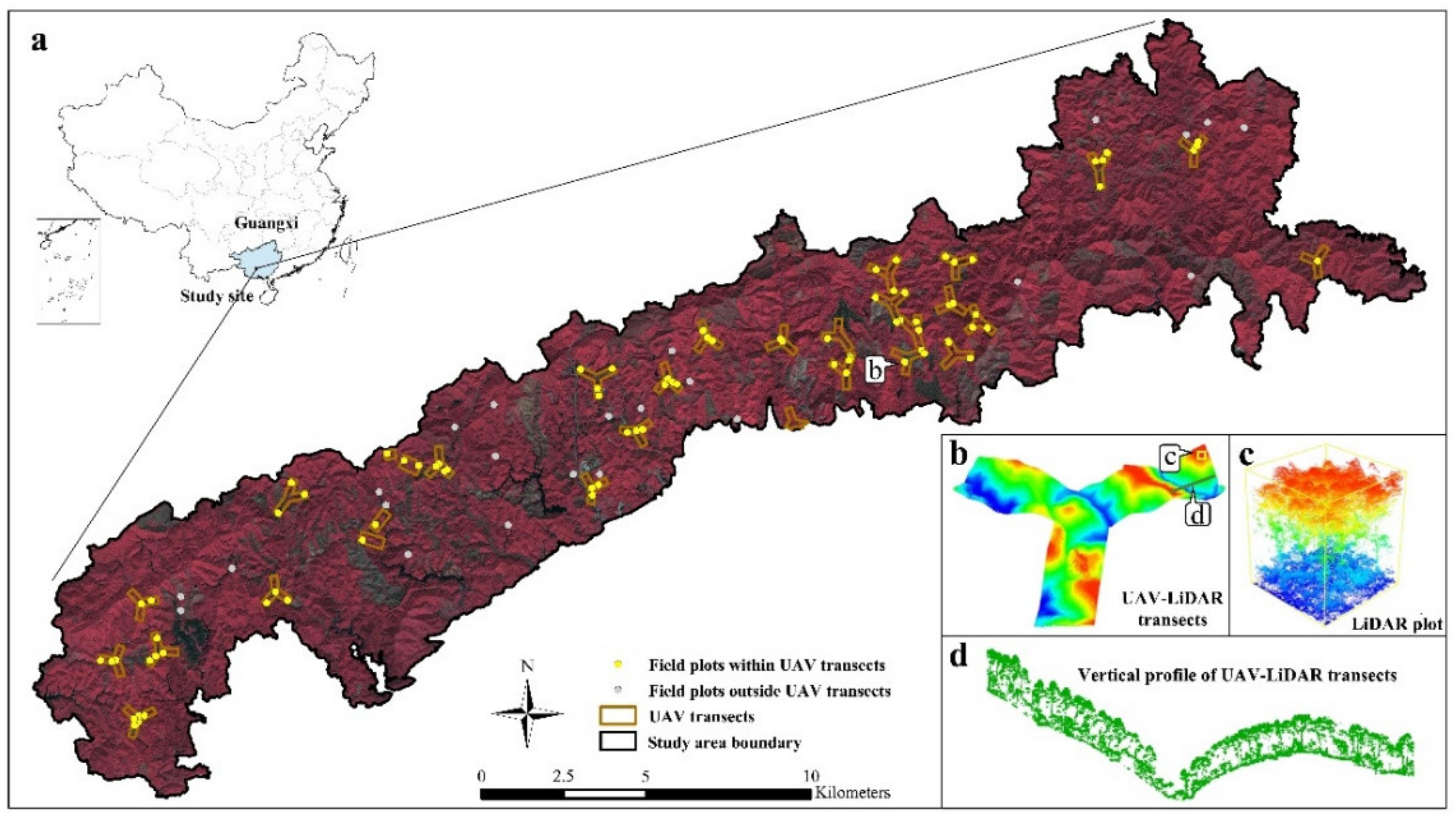
2.1. Study Area and Field Data

The study area covered 245 km² in the Gaofeng Forest Farm, Nanning city, Guangxi Province, southern China (108°8′–108°32′E, 22°50′–23°4′N) (Figure 1). The mean annual temperature was about 21 °C and mean annual precipitation was 1304 mm. Located in the humid subtropical monsoon climatic zone, it is suited for the growth of subtropical tree species. The relative elevation of the study area was about 80–460 m above sea level. The main planted forest species were Eucalypt (Eucalyptus robusta Smith), Chinese fir (Cunninghamia lanceolata (Lamb.) Hook.), Masson pine (Pinus massoniana Lamb.), Illicium verum (Illicium verum Hook.f.), etc.

The field survey was conducted between 25 December 2019 and 10 January 2020. Within the study area, we designed a total of 31 UAV sampling transects to acquire UAV-LiDAR data, depending on the distribution of tree species, stand age, and site quality. There were 49 field plots (for modeling) within the UAV-LiDAR transects and 25 field plots (for validation) outside the UAV-LiDAR transects (Figure 1). We surveyed two forest species, i.e., Eucalypt and Chinese fir. For all live trees (diameter at breast height (DBH) > 5 cm) in each plot, we recorded the tree species, DBH (using diameter tape), tree height (using Vertex IV hypsometer), crown diameter (using tape), and number of trees. The position of each plot center was measured by a Trimble R6 Global Navigation Satellite System with an accuracy of centimeter-level. In order to increase the representativeness of plots, additional 30 plots (for modeling) were extracted from normalized LiDAR transects using the random sampling principle, resulting in 104 square sample plots (20 × 20 m) in total. The point cloud segmentation (PCS) algorithm was used to detect individual trees and generate tree height [66]. DBH height formulas were then applied to calculate the DBH of each tree within plots for two species. Since DBH and height were measured, individual tree volume was generated by volume equations for two species and then stand volume was generated by summing individual tree volume within each plot. Finally, plot-level DBH, dominant height, volume, and stem density of inventory plots are summed in

Table 1. Summary of forest structural parameters that divided into modeling and validation plots.

Forest Structural Parameters	Modelling Plots (n = 79)		Validation Plots (n = 25)
	Mean	SD	Mean	SD
DBH (cm)	11.00	3.92	12.41	3.02
H (m)	17.61	6.53	19.99	1.94
V (m3·ha−1)	132.96	94.23	164.06	70.84
D (n·ha−1)	1391	594	1730	554

Note: DBH: mean DBH; H: dominant height; V: volume; D: stem density; SD: standard deviation.

.

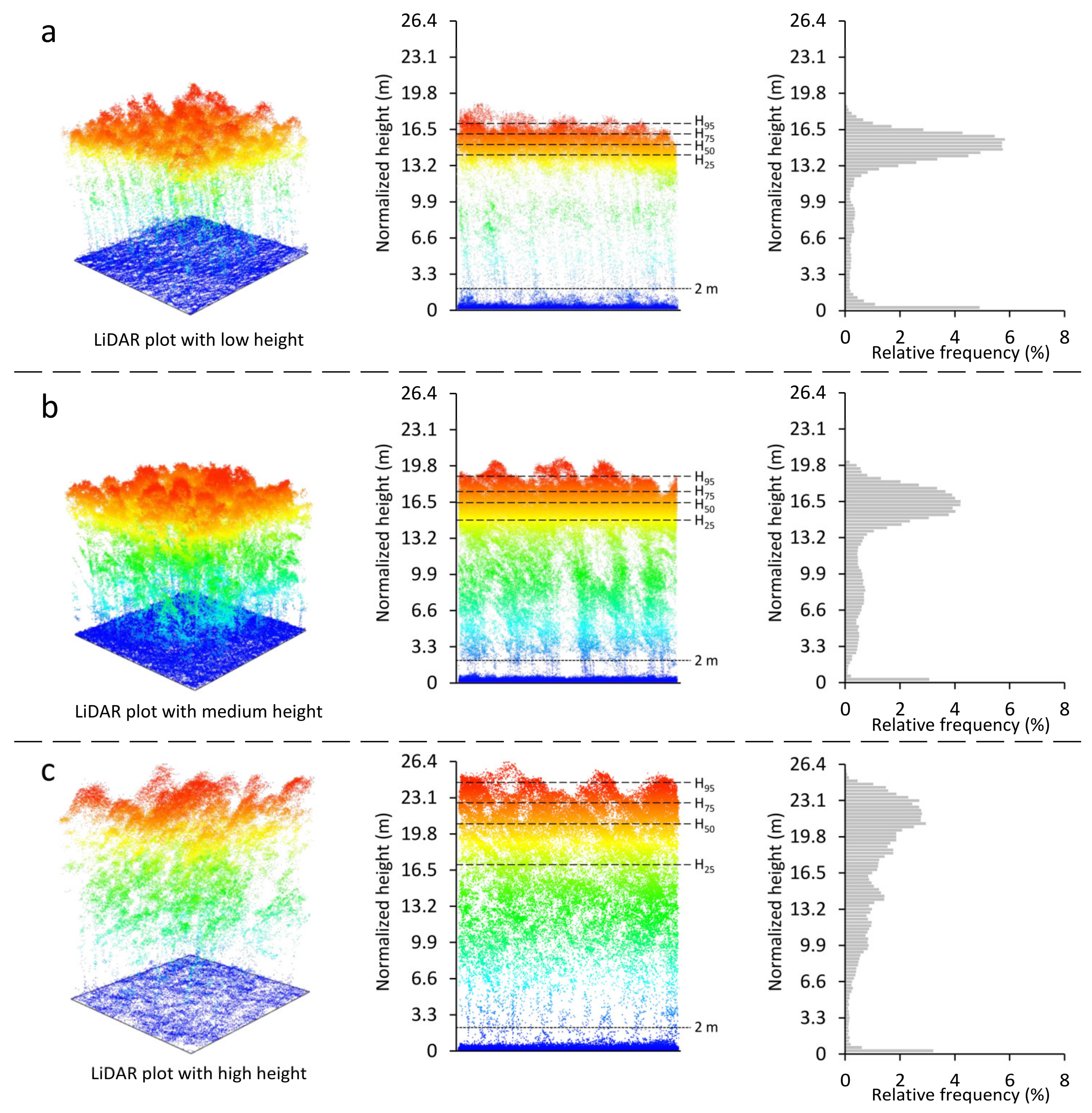
2.2. UAV System and UAV-LiDAR Data Processing

The LiAir 1350 UAV-LiDAR system (GreenValley, Beijing, China) equipped with Riegl VUX-1LR lightweight LiDAR sensor on the GV2000 multi-rotor UAV platform was used to collect UAV-LiDAR data from 23 May to 12 June 2020. Raw POS data were measured by the inertial measurement unit (IMU) and Global Navigation Satellite System (GNSS) modules. The flight altitude was 250 m above ground level. The flight speed was 7 m/s. The swath width was 200 m. The pulse repetition frequency was 200 kHz. The flight trajectories were pre-designed to cover all 31 UAV sampling transects for the advanced two-stage extrapolation analysis and then LiDAR data were obtained over approximately 9 km². The mean point density of pre-processed point clouds was about 340 pts·m⁻².

The pre-processing of raw UAV-LiDAR data mainly consisted of coordinate computation, strip alignment, point denoising, and point cloud normalization. The recorded UAV POS data and base station data were integrated to produce post-processed POS data and then calculate high-accuracy trajectories. LiDAR point clouds were georeferenced by the positioning data processed in LiGeoreference 3.2 software (GreenValley, Beijing, China). Strip alignment was then conducted for georeferenced point clouds of overlapping strips within each sampling region. Subsequently, the aligned georeferenced point clouds were denoised to remove the outliers detected by a Gaussian filter. A 0.5 m digital elevation model (DEM) was produced to normalize point clouds that were classified as ground points in LiDAR360 3.2 software (GreenValley, Beijing, China). Finally, normalized point clouds of sampling transects were generated and prepared for LiDAR metric extraction.

2.3. GF-6 Imagery Data Acquisition and Processing

Launched on 2 June 2018, GF-6 (Gaofen-6) was the sixth satellite of the high-definition Earth observation system (HDEOS) in China with high resolution and wide coverage. The GF-6 was equipped with one panchromatic and multispectral (PMS) camera and one multi-spectral wide-field view (WFV) sensor. PMS data had one 2 m panchromatic band and four 8 m multispectral bands (b1: 450–520 nm, b2: 520–590 nm, b3: 630–690 nm, and b4: 770–890 nm) across the imaging swath of 90 km. The GF-6 satellite imagery covered the study area and was acquired on 15 November 2019. The GF-6 PMS imagery was selected and processed by radiometric calibration, atmospheric correction, orthorectification, Gram-Schmidt spectral sharpening, and terrain correction in ENVI 5.3 software. A 4-band image with 2 m resolution was finally generated.

Subsequently, the imagery was co-registered to UAV-LiDAR with overall accuracy superior to 0.5 pixels. To do so, we set 30 ground control points (GCPs) for both UAV-LiDAR DEM and the imagery, mainly distributed in the roads within the study area, and then used them in the co-registration procedure. The extent polygons of the study area were then used to extract the imagery of the region of interest. Finally, the masked imagery was prepared for spectral index extraction and forest structural parameter estimation.

2.4. Metric Extraction and Selection from UAV-LiDAR and GF-6 Data

LiDAR metrics were calculated from normalized point clouds (

Table 2. A summary of LiDAR metrics obtained from UAV-LiDAR point clouds.

LiDAR Metrics	Description
Percentile heights (H25, H50, H75, H95)	Percentiles of canopy height distributions (25th, 50th, 75th, and 95th) > 2 m
Max height (Hmax)	Max of normalized point heights > 2 m
Minimum height (Hmin)	Min of normalized point heights > 2 m
Median height (Hmedian)	Average of normalized point heights > 2 m
Coefficient of variation of heights (Hcv)	Variation of normalized point heights >2 m
Canopy return density (D3, D5, D7, D9)	Proportion of points in each height interval (30, 50, 70, and 90) of total number of points.

). These metrics were proven effective for forest structural parameter estimation [67,68]. In order to remove the influence of low vegetation (e.g., grass and shrub), all LiDAR metrics were generated by removing the points below 2 m [69]. The variation of LiDAR plots with various tree heights, as well as the height percentiles and vertical distribution of point clouds, is presented in Figure 2.

Plot-level GF indices were derived from processed GF-6 imagery (

Table 3. A summary of GF metrics derived from GF-6 imagery.

GF Indices	Variable	Equation	Description	Reference
Spectral indices	R, G, B, NIR	B1, B2, B3, B4	GF-6 bands	-
	ARVI	(B4 − (B3 − (B1 − B3)))/ (B4 + (B3 − (B1 − B3)))	Atmospherically resistant vegetation index	[72]
	CVI	B4 × B3/(B22)	ChlorophyII vegetation index	[73]
	DVI	B4 − B3	Difference vegetation index	[74]
	EVI	2.5 × (B4-B3)/ (B4 + 6 × B3 − 7.5 × B1 + 1)	Enhanced vegetation index	[75]
	EVI2	2.5 × (B4 − B3)/ (B4 + 2.4 × B3 + 1)	Enhanced vegetation index 2	[76]
	GDVI	(B42 − B32)/(B42 + B32)	Generalized difference vegetation index	[77]
	NDVI	(B4 − B3)/(B4 + B3)	Normalized difference vegetation index	[78]
	NDWI	(B2 − B4)/(B2 + B4)	Normalized difference water index	[78]
	NLI	(B42 − B3)/(B42 + B3)	Non-linear vegetation index	[79]
	RVI	B4/B3	Ratio vegetation index	[80]
	SAVI	1.5 × (B4 − B3)/(B4 + B3 + 0.5)	Soil-adjusted vegetation index	[81]
Texture indices	Mean, variance, homogeneity, contrast, dissimilarity, entropy, second moment, correlation		GLCM texture measures (window size: 3 × 3, 5 × 5, 7 × 7)	[82]

). In addition to four original bands, spectral indices and texture indices were also derived to estimate forest structural parameters [70,71]. Spectral feature transformations to extract vegetation indexes were performed, as well as principal component analysis (PCA). Then, eight texture indices were extracted from the first principal component of PCA with three window sizes (3 × 3, 5 × 5, and 7 × 7) at an offset ([1,1]) and a 64 gray level quantization.

2.5. Forest Structural Parameter Estimation Procedure

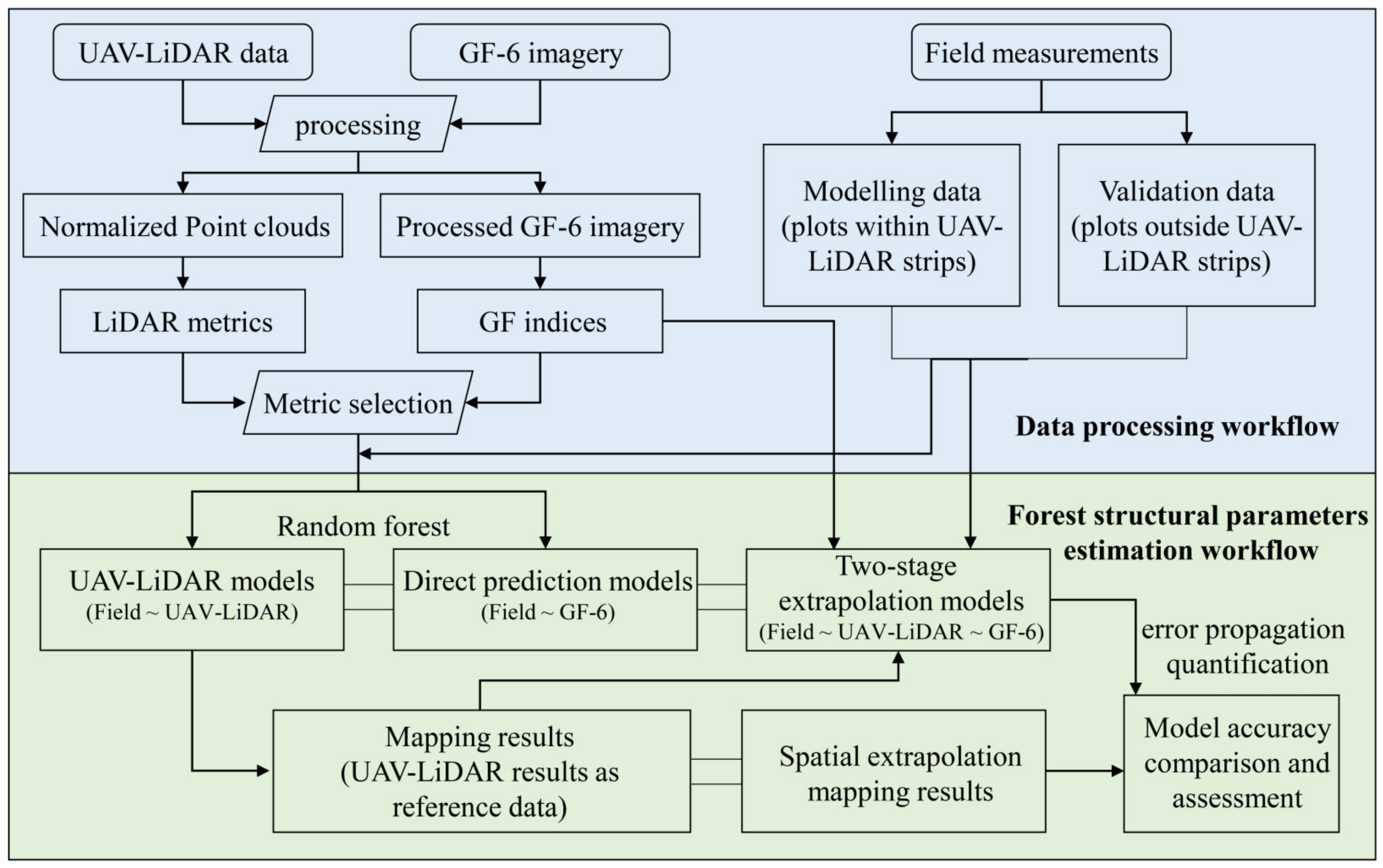
2.5.1. Data Processing Workflow

First, raw UAV-LiDAR data and GF-6 imagery were pre-processed, and then used to extracted LiDAR metrics (Table 2) and GF indices (Table 3). All inventory plots were divided into modeling plots and validation plots according to the position within or outside the UAV-LiDAR transects. The quantification of error propagation was specially utilized to assess the uncertainty through the two-stage extrapolation procedure. Figure 3 shows the workflow of data processing and forest structural parameter estimation.

2.5.2. Variable Selection

The variable selection within a large subset of predictor metrics is critical to model accuracy due to its ability to eliminate uncorrelated and non-redundant variables, reducing model complexity and accelerating model training time [83]. A total of 15 LiDAR metrics and 39 GF indices were analyzed with the Boruta variable selection algorithm using the ‘Boruta’ R package [84]. The Boruta algorithm is a wrapper based on the random forest classification algorithm. It uses a random forest approach to extract features and compute their importance by shuffling their order [84]. Figure 4 shows the variable importance results using different models.

2.5.3. Random Forest Algorithm

Random forest (RF) is a commonly used machine learning algorithm developed by Breiman [85]. Its ease of use and flexibility in handling both classification and regression problems have fueled its adoption. It has been widely used in forest structural parameter estimation applications with remote sensing data and has achieved good performance [86,87,88]. Each tree was generated independently from a random sub-sample of data (two-thirds), and the remaining one-third of sub-samples was used for out-of-bag error estimation. For each tree node, a subset of predictors was used to identify the best split. The final estimation results were from average prediction values of the individual trees with low bias and high variance [85].

Two important parameters were set: (1) ntree that determined the total number of decision tress; (2) mtry that represented input variable numbers at each node. We implemented the “random forest” package in R to build estimation models in combination with field plots or LiDAR samples and metrics [85]. In this study, ntree equaled 500, and mtry equaled $\sqrt{n_{mtry}}$ in which n was defined as the number of input variables.

2.5.4. Advanced Two-Stage Extrapolation Approach

In this study, we established an advanced two-stage extrapolation approach for forest structural parameter estimation. Error propagation through the spatial extrapolation procedure was specially considered to quantify the uncertainty of model predictions. The two-stage procedure included generating high-accuracy UAV-LiDAR mapping results and linking the relationships between mapping products and field plots. The advanced two-stage extrapolation approach depended on statistical models and the ABA method to estimate and map forest structural parameters.

First, LiDAR metrics were generated to model and map forest structural parameters with field plots. All field plots and corresponding metrics were randomly split into modeling data and validation data in a proportion of 8:2 (

Table 4. Summary of modeling and validation plots of four forest structural parameter estimation models.

Estimation Models	Modelling Data	Validation Data
UAV-LiDAR models (Field~UAV-LiDAR)	63 field plots	16 field plots
Direct prediction models (Field~GF-6)	63 field plots	16 field plots
Two-stage extrapolation models (Field~UAV-LiDAR~GF-6)	21,123 LiDAR sample plots	25 field plots outside UAV-LiDAR transects

). RF was conducted to build estimation models with modeling data, whereas validation data were used to assess the estimation accuracy. The estimation accuracy represented final results of UAV-LiDAR models. Then, the estimation models were spatially extrapolated to all UAV-LiDAR grid cells to generate UAV-LiDAR mapping results with a resolution of 20 m.

Second, UAV-LiDAR mapping results were then used as reference data to calibrate wall-to-wall satellite imagery. In this step, UAV-LiDAR mapping products were considered as intermediate data to bridge field plots and satellite imagery. Reference data and corresponding GF metrics of each grid cell were modeled using the RF algorithm with the same parameter settings as the UAV-LiDAR models. A total of 21,123 UAV-LiDAR sample plots were utilized and 25 field plots outside the UAV-LiDAR transects were used to validate the model accuracy. Thus, large area forest structural parameter mapping results were generated with the full-coverage of GF-6 imagery. The summary of modeling plots and validation plots of different forest structural parameter estimation models are presented in Table 4.

Error propagation through the extrapolation procedure was assessed to quantify the uncertainties of estimation models. The uncertainty quantification of RF regression predictions can be assessed by several approaches: the jackknife-after-bootstrap approach [89], U-statistics approach [90], Monte Carlo simulation approach [91], and quantile regression forests (QRF) approach [92]. The U-statistics approach was proposed on the mathematical foundations of the U-statistic with asymptotic normality. It can be used to estimate the variance of RF prediction and make it possible to generate pixel-level uncertainty maps.

We selected the U-statistics approach as the base algorithm to generate spatial extrapolation-specific uncertainty analysis. In this study, we dismissed the uncertainty related with tree allometric models due to the findings of McRoberts and Westfall [93]. Mentch and Hooker [90] developed formal statistical inference procedures for supervised ensemble predictions such as RF under the asymptotic normality of U-statistics. By averaging over trees built on strict sub-samples of the training sets, they demonstrated the asymptotical normality of RF. Uncertainty of RF prediction was then quantified by calculating U-statistic variance parameters that were used to estimate the variance of a RF prediction.

The U-statistics allow a minimum variance unbiased estimator to be obtained from each unbiased estimator of an estimator parameter for large classes of probability distributions [94]. The “U” in U-statistics stands for unbiased. An unbiased estimator of a statistic can be derived by calculating the average of possible results of sub-samples. Let $Z_1,\dots ,Z_r$ be observation pairs and let $\theta$ be a statistic or population parameter of interest. Suppose that an unbiased estimator $h$ of $\theta$ exists with $r\le n$ arguments, where its expected value equals $\theta$, denoted by Equation (1):

$$\theta =E\left[h\left(Z_1,\dots ,Z_r\right)\right]$$

(1)

Postulating that the expected value $\theta$ is unbiased approximated, a total of $\left(\begin{array}{c}n\\ r\end{array}\right)$ sub-samples of size $r$ are selected from the original sample $Z$ that has size $n$ [95]. The minimum variance unbiased estimator for $\theta$ is given as a U-statistic with kernel $h$ and rank $r$ in Equation (2):

$$U_n=\frac{1}{\left(\begin{array}{c}n\\ r\end{array}\right)}{\displaystyle \sum }_i^{\left(\begin{array}{c}n\\ r\end{array}\right)}h\left(Z_{i1},\dots ,Z_{ir}\right)$$

(2)

RF has additional randomness caused by the random selection of the split at each node in each tree. Random perturbation parameters $\left\{w_i:i\in 1,\dots ,m_n\right\}$ should be considered into U-statistics to make the mean prediction $U_{w;n,r_{n,m_n}}^{\psi \left(x_0\right)}$ asymptotically normal, and these parameters are independently selected of the original sample $Z_1,\dots ,Z_r$. The random kernel U-statistic for RF predictions is denoted in Equation (3):

$$U_{w;n,r_{n,m_n}}^{\psi \left(x_0\right)}=E_w[\frac{1}{m_n}{\displaystyle \sum }_i^{m_n}{f}_{x_0,r_n}^{{\psi }_i;w_i}\left(Z_{i1},\dots ,Z_{i{r}_n}\right)]$$

(3)

The variance of the expected RF prediction can be estimated due to the asymptotic normality of U-statistics. Lee [94] described the variance value ${\eta }_{c,r_n}$ of the expected prediction of the samples that contained $c$ elements inconsistent with each other in Equation (4):

$${\eta }_{c,r_n}=var\left(\left.E(h_{r_n}\left(Z_1,\dots ,Z_{r_n}\right) \right| Z_1=z_1,\dots ,Z_c=z_c\right))$$

(4)

Mentch and Hooker [90] estimated the variance value ${\widehat{\eta }}_{c,r_n}$ of RF predictions by selecting several sub-samples of size $r_n$ from the training set, building a tree with each sub-sample, and averaging the sub-sample predictions. To estimate the variance ${\widehat{\eta }}_{c,r_n}$, $c$ observations ${\tilde{z}}_1,\dots ,{\tilde{z}}_c$ were selected from the raw training set as initial fixed points. A certain number of Monte Carlo simulations $m_n$ denoted the number of sub-samples. ${\tilde{z}}^j$ denoted the jth set of fixed points and $S_{\tilde{z}\left(j\right),i}$ denoted the ith sub-sample that included ${\tilde{z}}^j$ of the tree function $f_{x_0,r_n}^{{\psi }_i}$ in Equation (5).

$${\widehat{\eta }}_{c,r_n}=var[\frac{1}{m_n}{{\displaystyle \sum }}_{i=1}^{m_n}{f}_{x_0,r_n}^{{\psi }_i}\left(S_{\tilde{z}\left(1\right),i}\right),\dots ,\frac{1}{m_n}{{\displaystyle \sum }}_{i=1}^{m_n}{f}_{x_0,r_n}^{{\psi }_i}\left(S_{\tilde{z}\left(n_{\tilde{z}}\right),i}\right)]$$

(5)

For the final variance estimate, the case $c=1$ and $c=r_n$ need to be calculated. By adding corrected ${\widehat{\eta }}_{1,r_n}$ (i.e., $\frac{r_n^2}{(\frac{n}{m_n})}{\widehat{\eta }}_{1,r_n}$) and ${\widehat{\eta }}_{r_n,r_n}$, detailed descriptions are shown in Equation (6).

$$var\left(U_{w;n,r_{n,m_n}}^{\psi \left(x_0\right)}\right)=\frac{r_n^2}{(\frac{n}{m_n})}{\widehat{\eta }}_{1,r_n}+{\widehat{\eta }}_{r_n,r_n}$$

(6)

The value of $m_n$ and $n_{\tilde{z}}$ were chosen as appropriate. Generally speaking, a larger value of the Monte Carlo sub-samples $m_n$ is necessary for accurate precision while the number of initial fixed points $n_{\tilde{z}}$ needed is smaller. In the spatial extrapolation uncertainty analysis procedure, we used an $m_n$ of 1000 and $n_{\tilde{z}}$ of 10. In this study, the uncertainty $\epsilon$ was the square root of the final variance estimate in Equation (7):

$$\epsilon =\sqrt{var\left(U_{w;n,r_{n,m_n}}^{\psi \left(x_0\right)}\right)}$$

(7)

Now that the uncertainty calculation method of RF has been defined, we can further apply it to the spatial extrapolation procedure to quantify the error propagation within the process. We estimated UAV-LiDAR mapping results ${\mathrm{LiDAR}}_{pix}^n$ using RF in Equation (8), and error ${\mathsf{\epsilon }}_{pix, LiDAR}$ of the first stage (from field plots to UAV-LiDAR) of the spatial extrapolation procedure was calculated using Equation (9).

$${\mathrm{LiDAR}}_{pix}^n=RF(fiel{d}_{pix}^n,LiDA{R}_{metrics})$$

(8)

$${\mathsf{\epsilon }}_{pix, LiDAR}=\sqrt{\mathrm{var}{\left({\mathrm{U}}_{w;n,r_{n,m_n}}^{\psi \left(x_0\right)}\right)}_{field~LiDAR}}$$

(9)

Then, we propagated error ${\mathsf{\epsilon }}_{pix, LiDAR}$ to LiDAR estimates and generated ${\widehat{\mathrm{LiDAR}}}_{pix}^n$ using normally distributed random values in Equation (10):

$${\widehat{\mathrm{LiDAR}}}_{pix}^n={\mathrm{LiDAR}}_{pix}^n\times (1+{\mathsf{\epsilon }}_{pix, LiDAR}\times X_{pix}^n)$$

(10)

where the symbol ^ denotes LiDAR estimates that included the estimated error, $n$ is the number of Monte Carlo simulations, and $pix$ is one pixel. $X$ is a random number under a normal distribution $X$~N(0,1).

At the second stage (i.e., from UAV-LiDAR estimates to GF-6), GF mapping results ${\widehat{\mathrm{GF}}}_{pix}^n$ were calculated using Equation (11) with ${\widehat{\mathrm{LiDAR}}}_{pix}^n$ and GF metrics $G{F}_{metrics}$ using RF. In this stage, first stage error ${\mathsf{\epsilon }}_{pix, LiDAR}$ of each pixel was propagated to GF estimates and generated final error ${\epsilon }_{pix,upscaling}$ through the spatial extrapolation procedure in Equation (12):

$${\widehat{\mathrm{GF}}}_{pix}^n=RF({\widehat{\mathrm{LiDAR}}}_{pix}^n,G{F}_{metrics})$$

(11)

$${\epsilon }_{pix, upscaling}=\sqrt{var{\left(U_{w;n,r_{n,m_n}}^{\psi \left(x_0\right)}\right)}_{LiDAR~GF}}$$

(12)

2.6. Sensitivity Analysis by Reducing UAV-LiDAR Point Density and Sampling Intensity

Point density is highly related to data acquisition cost [96,97]. Reducing point density of UAV-LiDAR reduces costs and improves computing efficiency for large area forest structural parameter estimations. In addition to acquisition cost, computational challenges should be considered for building the statistical relationship between UAV-LiDAR mapping grid cells and corresponding metrics while using the advanced two-stage extrapolation approach. Each grid cell was used to represent one UAV-LiDAR plot, and corresponding GF metrics of each grid cell were extracted at the same time for modeling, which influences computational efficiency.

Therefore, sensitivity analysis of the effects of point density and sampling intensity on forest structural parameter estimation was indispensable. For sensitivity analysis of point density, point cloud data were extracted ranging from raw point density (340 pts·m⁻²) to lower point density. It included 80% (272 pts·m⁻²), 60% (204 pts·m⁻²), 40% (136 pts·m⁻²), 20% (68 pts·m⁻²), 10% (34 pts·m⁻²), and 1% (3 pts·m⁻²) using the “subsampling” method in LiDAR360 3.2 software (GreenValley, Beijing, China). By setting the sampling rate, the algorithm randomly retained the specified number of points to decimate point density. For the sensitivity analysis of sampling intensity, raw UAV-LiDAR mapping grid cells (i.e., UAV-LiDAR plots) were randomly eliminated 10% at one time to compare the estimation results with different sampling intensities. The mapping results were generated from undecimated original UAV-LiDAR point clouds (340 pts·m⁻²). The sampling intensity ranged from 100% to 10% of the original data, and the UAV-LiDAR plots ranged from 21,123 to 2112.

Forest structural parameter estimation models were then built and validation results were recorded to be used for accuracy comparison.

2.7. Model Evaluation and Accuracy Assessment

The two-stage extrapolation models were developed and mapping results were generated to provide the extrapolation of structural parameters. To assess and compare the accuracy of two-stage extrapolation models, UAV-LiDAR models that rely on LiDAR metrics and field plots were evaluated, as well as direct prediction models that rely on GF-6 metrics and field plots.

To assess the model accuracy, different validation data were utilized for UAV-LiDAR models, direct prediction models, and two-stage extrapolation models using R², RMSE, and rRMSE [98] using Equations (13)–(15).

$$R^2=1-\frac{{{\displaystyle \sum }}_{i=1}^n{(x_i-{\widehat{x}}_i)}^2}{{{\displaystyle \sum }}_{i=1}^n{(x_i-{\overline{x}}_i)}^2}$$

(13)

$$RMSE=\sqrt{\frac{1}{n}{\displaystyle \sum }_{i=1}^n{(x_i-{\widehat{x}}_i)}^2}$$

(14)

$$rRMSE=\frac{RMSE}{\overline{x}}\times 100\%$$

(15)

where $x_i$ is field measurement;$\overline{x_i}$ is the mean field measurement;${\widehat{x}}_i$ is the estimated value; $\overline{x}$ is the mean field measurement; $p$ is the metrics number; $i$ is the plot ID; and $n$ is the plot number.

3. Results

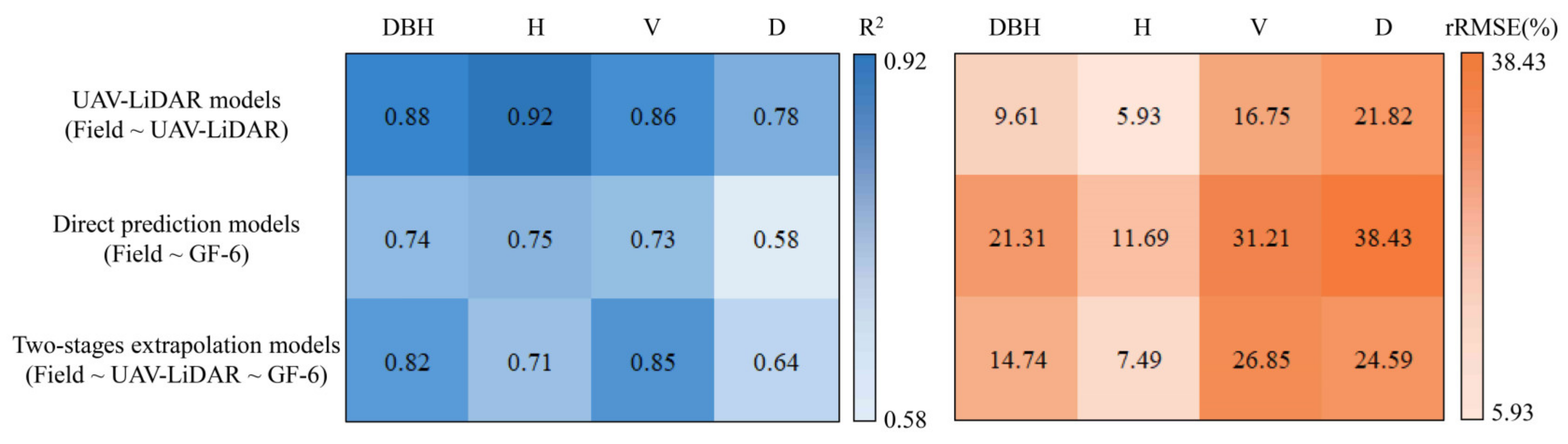
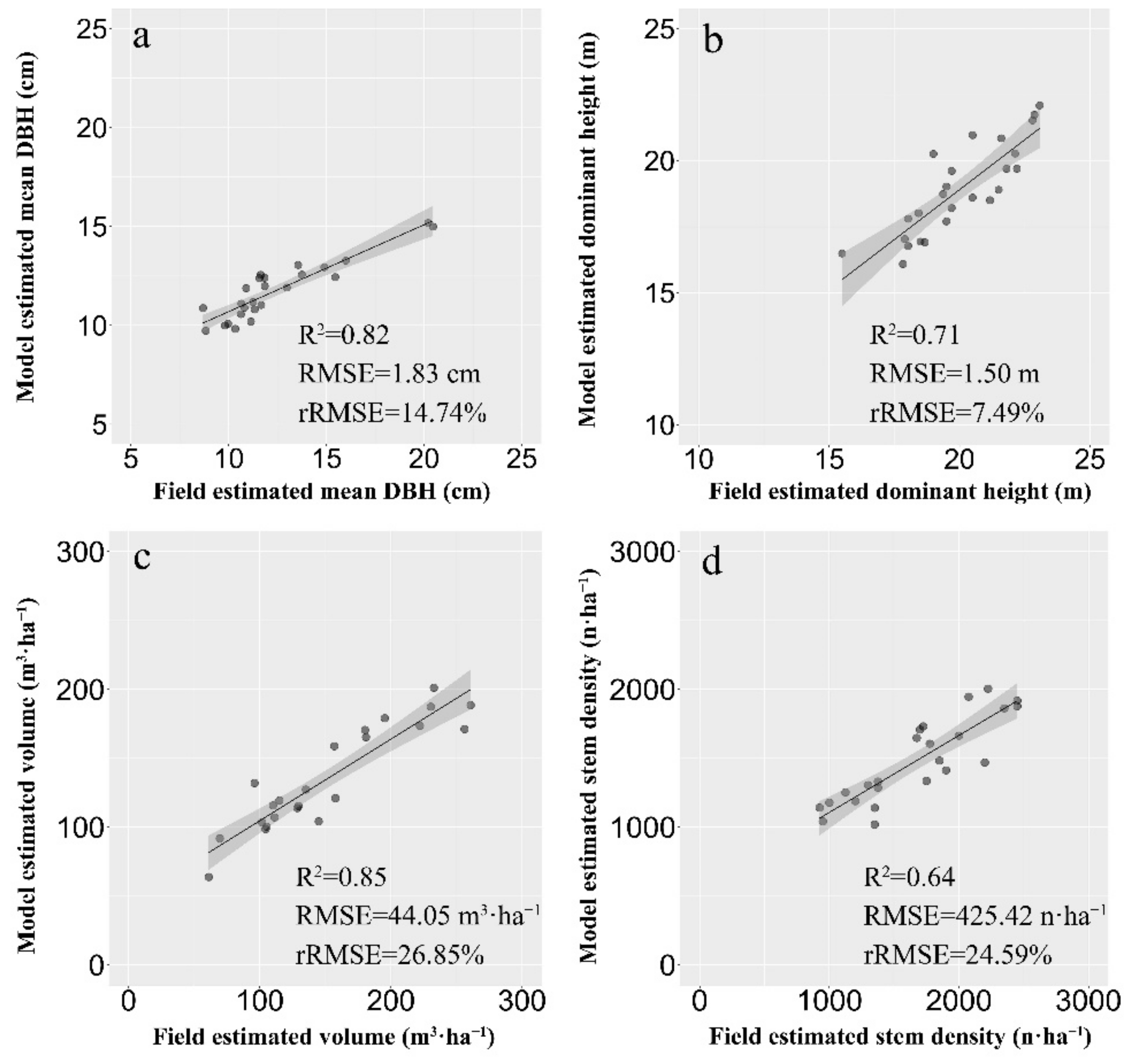
3.1. Comparison of Different Forest Structural Parameter Estimation Models

To test the effectiveness and capability of the advanced two-stage extrapolation approach, UAV-LiDAR models (Field~UAV-LiDAR) and direct prediction models (Field~GF-6) were generated to compare forest structural parameter estimation accuracy with two-stage extrapolation models (Field~UAV-LiDAR~GF-6) in terms of R² and rRMSE for mean DBH, dominant height, volume, and stem density. According to variable importance results (Figure 4), metrics were derived to build estimation models with field plots. Figure 5 shows the comparison of model estimation results. In this study, UAV-LiDAR models were built at the stand scale and were considered as intermediate data to bridge field plots and GF-6 imagery. Two-stage extrapolation models and direct prediction models were built at the landscape scale, and estimation results showed that two-stage extrapolation models had higher accuracy than direct prediction models.

For different estimation models, UAV-LiDAR models obtained the best estimation accuracy (R² = 0.78–0.92, rRMSE = 5.93–21.82%) at the stand scale. In general, two-stage extrapolation models (R² = 0.64–0.85, rRMSE = 7.49–26.85%) performed better than direct prediction models (R² = 0.58–0.75, rRMSE = 11.69–38.43%) at the landscape scale. Dominant height had the highest estimation accuracy (R² = 0.71–0.92, rRMSE = 5.93–11.69%), whereas mean DBH (R² = 0.74–0.88, rRMSE = 9.61–21.31%), volume (R² = 0.73–0.86, rRMSE = 16.75–31.21%), and stem density (R² = 0.58–0.78, rRMSE = 21.82–38.43%) had lower accuracies.

Figure 6 shows the scatterplots of field plots and two-stage extrapolation model estimated results to which validation plots were applied to assess the model results. Dominant height demonstrated the highest estimation accuracy (R² = 0.71, RMSE = 1.50 m, rRMSE = 7.49%), and mean DBH exhibited good performance (R² = 0.82, RMSE = 1.83 cm, rRMSE = 14.74%). Stem density (R² = 0.64, RMSE = 425.42 n·ha⁻¹, rRMSE = 24.59%) and volume (R² = 0.85, RMSE = 44.05 m³·ha⁻¹, rRMSE = 26.85%) demonstrated relatively lower accuracy than the other two estimation models.

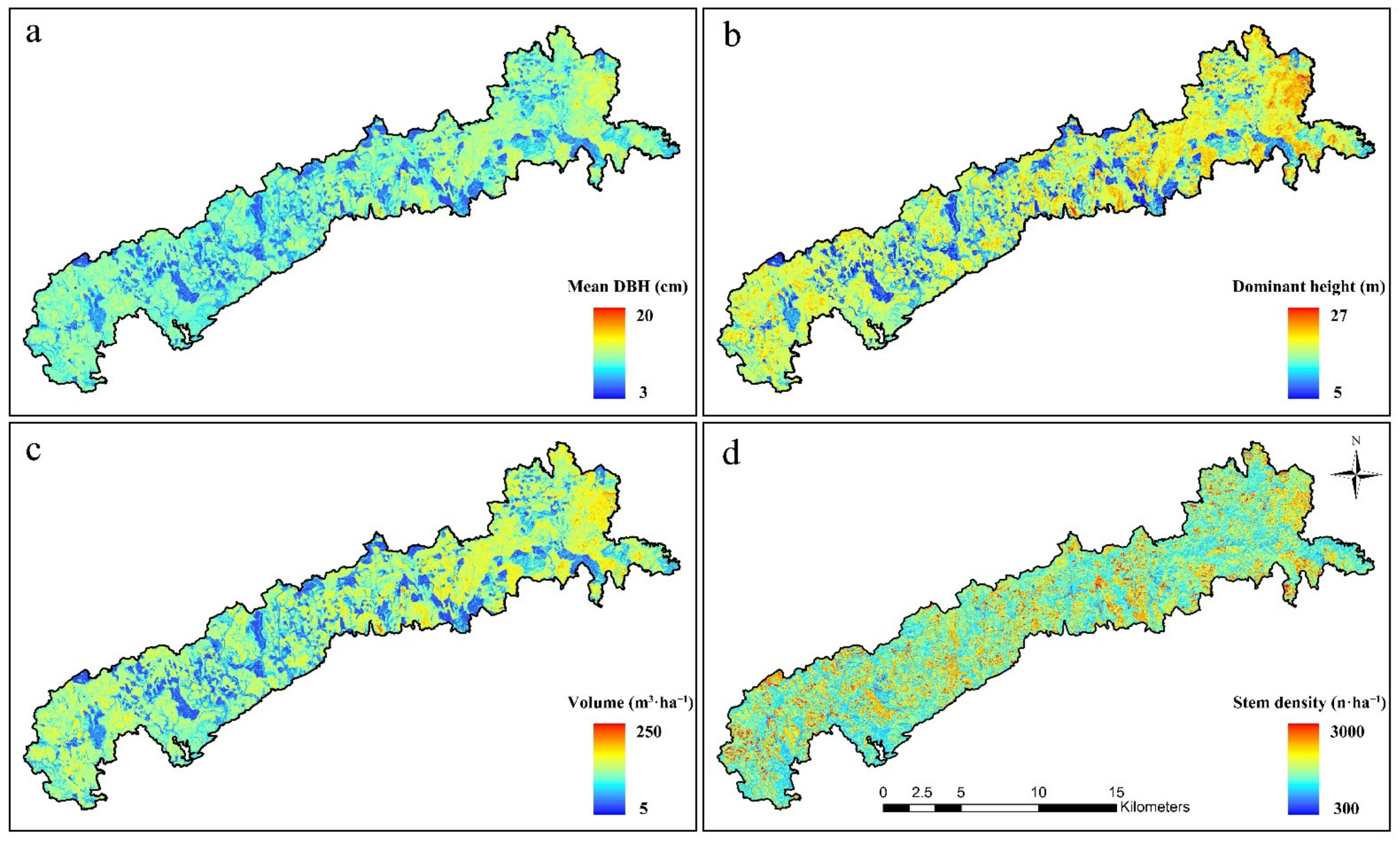
3.2. Maps of Forest Structural Parameters Using the Advanced Two-Stage Extrapolation Approach

In this study, low-cost, high-precision, and large area spatially extrapolated forest structural parameter mapping products were generated. We used the UAV-LiDAR estimation models (Figure 5) to generate UAV-LiDAR transect mapping products, then two-stage extrapolation models and extrapolation results were generated. The extrapolation results of forest structural parameters predicted by the advanced two-stage extrapolation approach are shown in Figure 7. Blue indicates a lower value and red indicates a higher value. The spatial patterns of mean DBH, dominant height, and volume indicated similar trends. It was indicated that the upper right part of the study area had higher values than the bottom left for Figure 7a–c. The mapping of stem density is shown for Figure 7d.

3.3. Sensitivity of Estimation Results by Reducing UAV-LiDAR Point Density

To assess the effects of point density, raw point clouds were decimated from 100% (original) to 1%. Forest structural parameter estimation models were separately built and the validation results are presented in

Table 5. Sensitivity analysis of estimation results by reducing UAV-LiDAR point density.

Forest Structural Parameters	Evaluation	100% (340 pts·m−2)	80% (272 pts·m−2)	60% (204 pts·m−2)	40% (136 pts·m−2)	20% (68 pts·m−2)	10% (34 pts·m−2)	1% (3 pts·m−2)
DBH (cm)	R2	0.82	0.81	0.79	0.77	0.71	0.65	0.58
	RMSE	1.83	1.92	1.88	1.91	1.94	2.11	2.88
	rRMSE	14.74%	15.50%	15.15%	15.35%	15.67%	17.03%	23.22%
H (m)	R2	0.71	0.68	0.68	0.69	0.68	0.63	0.62
	RMSE	1.50	1.70	1.78	1.64	1.72	1.75	1.96
	rRMSE	7.49%	8.49%	8.92%	8.23%	8.62%	8.78%	9.79%
V (m3·ha−1)	R2	0.86	0.84	0.82	0.80	0.80	0.69	0.61
	RMSE	44.05	45.36	46.16	46.09	45.84	51.51	55.52
	rRMSE	26.85%	27.65%	28.13%	28.09%	27.95%	31.39%	33.84%
D (n·ha−1)	R2	0.64	0.60	0.56	0.55	0.52	0.45	0.40
	RMSE	425.42	479.30	468.75	466.34	478.76	533.28	539.62
	rRMSE	24.59%	27.71%	27.10%	26.95%	27.67%	30.83%	31.19%

. In general, the accuracy of each prediction model decreased in varying degrees as point density decreased. In general, the results showed relatively stable and acceptable estimation accuracy for 10% point density (34 pts·m⁻²). The model results of mean DBH ranged from R² = 0.82, rRMSE = 14.74% to R² = 0.58, rRMSE = 23.22%. The model results of dominant height ranged from R² = 0.71, rRMSE = 7.49% to R² = 0.62, rRMSE = 9.79%. The model results of volume ranged from R² = 0.86, rRMSE = 26.85% to R² = 0.61, rRMSE = 33.84%. The model results of stem density ranged from R² = 0.64, rRMSE = 24.59% to R² = 0.40, rRMSE = 31.19%. For all forest structural parameters, the prediction accuracy of dominant height was least affected by the decimation of point density (ΔR² = 0.09, ΔrRMSE = 2.30%) which reflected the stable prediction ability. Compared to dominant height, mean DBH indicated greater impacts (ΔR² = 0.24, ΔrRMSE = 8.48%), as well as volume (ΔR² = 0.25, ΔrRMSE = 6.99%) and stem density (ΔR² = 0.24, ΔrRMSE = 6.60%).

3.4. Sensitivity of Estimation Results by Reducing UAV-LiDAR Sampling Intensity

The sensitivity analysis of sampling intensity results are shown in Figure 8. Overall, there were downward trends for model accuracy of all forest structural parameters as UAV-LiDAR sampling intensity decreased from 100% to 10%. In general, the results showed relatively stable and acceptable estimation accuracy for 20% of sampling intensity. There was a sudden drop in the curves for mean DBH and dominant height models when sampling intensity decreased from 20% to 10%. A similar phenomenon appeared for volume models when sampling intensity decreased from 30% to 10%. It appeared for stem density models when sampling intensity decreased from 80% to 70%.

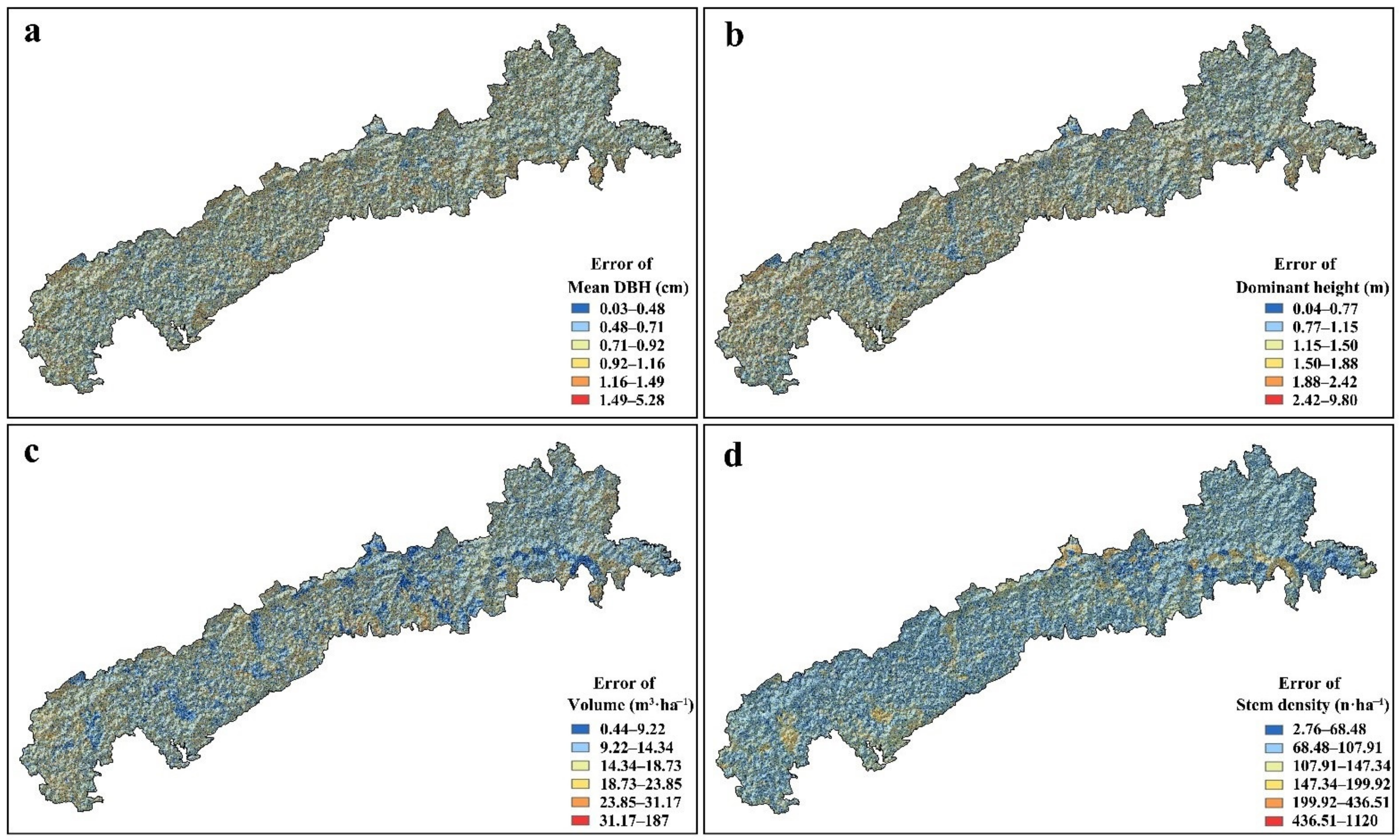
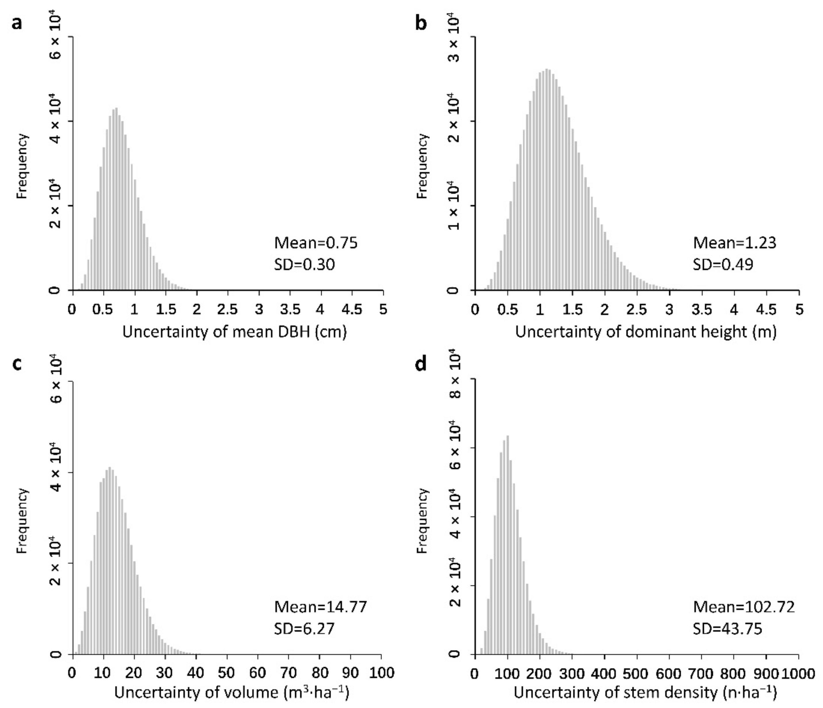
3.5. Error Propagation Analysis through the Advanced Two-Stage Extrapolation Approach

To understand error propagation through the extrapolation procedure, we utilized the modified U-statistics uncertainty approach to generate an advanced two-stage extrapolation specific uncertainty analysis approach. The proposed approach was then used to quantify pixel-level estimates’ uncertainty and generate uncertainty maps of forest structural parameters (Figure 9). Due to the asymptotic normality of the U-statistic of RF error, all pixels of forest structural parameter uncertainty maps were used to generate histograms (Figure 10). The histograms indicated that the pixel-level average value of uncertainty was 0.75 cm for mean DBH, 1.23 m for dominant height, 14.77 m³·ha⁻¹ for volume, and 102.72 n·ha⁻¹ for stem density. The pixel-level standard deviation value of uncertainty was 0.30 cm for mean DBH, 0.49 m for dominant height, 6.27 m³·ha⁻¹ for volume, and 43.75 n·ha⁻¹ for stem density.

4. Discussion

Accurate estimation and extrapolation of forest structural parameters in planted forests in broader landscapes is of great value for characterizing forest structure, grasping spatial distribution status, and responding to precision silviculture. This study performed an advanced two-stage extrapolation approach by using UAV-LiDAR data as bridging data to connect field plots and satellite imagery. The approach was established to generate extrapolation mapping of forest structural parameters.

In addition, to further explore the relationship between estimation accuracy and UAV-LiDAR point density and sampling intensity, sensitivity analysis was conducted. The main contributions of this study are: (1) exploring the feasibility of the advanced two-stage extrapolation approach that combined UAV-LiDAR and GF-6 satellite imagery; (2) assessing the capacity of the advanced two-stage extrapolation approach for estimating forest structural parameters and spatial distribution mapping in southern China; (3) examining how well point density and sampling intensity influenced the estimation accuracy; and (4) quantifying error propagation through the spatial extrapolation procedure.

4.1. Remote Sensing Data

The advanced two-stage extrapolation approach provided a practical solution that relied on the combination of UAV-LiDAR data and GF-6 satellite imagery to estimate forest structural parameters in broader landscapes in this study. LiDAR was an effective technology to characterize forest canopy structures and estimate forest structural parameters due to its advantages to detect horizontal and vertical information of forests [11,57]. Additionally, 3-D point clouds generated from UAV-based digital aerial photogrammetry provided detailed information of the forest canopy and have been proven useful for estimating forest structural parameters [49,99]. Considering the advantages of low cost and easy access, high-resolution UAV-LiDAR or UAV-DAP data may be promising for bridging data in spatial extrapolation studies. For instance, Puliti et al. (2018) [100] estimated forest growing stock volume using hierarchical model-based inference that combined UAV-DAP and Sentinel-2 auxiliary data. They demonstrated the feasibility of UAV and Sentinel-2 satellite imagery for large-scale forest inventory.

Apart from UAV-LiDAR or UAV-DAP, bridging data can be acquired from different types of platforms, such as backpack and mobile LiDAR, airborne LiDAR, and spaceborne LiDAR [101]. They collect data in the form of LiDAR transects that provide partial-coverage observations for a large area. In combination with spatial continuous satellite imagery, complete coverage forest structural parameters may be estimated. Li et al. (2015) [102] utilized airborne LiDAR to bridge field and satellite-based measurements to estimate landscape forest AGB. Su et al. (2017) [103] mapped forest tree height by coupling field plots, airborne LiDAR, GLAS data, optical imagery, and topographic and climate data. They demonstrated good performance of the GLAS tree height product as intermediate data for a wall-to-wall tree height map in broader landscapes. With the development of satellite technology, VHSR satellite imagery (e.g., Sentinel, Gaofen) or LiDAR (e.g., GEDI, ICESat-2) provide the potential to improve the extrapolation ability for forest structural parameters because of their global coverage and increased relevance signals [54]. In future works, various novel remote sensing data may be examined for the ability for large area forest structural parameter estimation and mapping.

4.2. UAV-LiDAR Point Density and Sampling Intensity

The UAV-LiDAR point density affected data acquisition cost that may be caused by different LiDAR sensors, flight height, and flight time [51,52]. Sampling intensity from UAV-LiDAR mapping grid cells influenced computation time and forest structural parameter estimation accuracy [55], as well as UAV-LiDAR coverage. Hence, reducing UAV-LiDAR point density and sampling intensity needs to be considered to balance data acquirement cost and estimation accuracy. This study examined how point density and sampling intensity affect the estimation accuracy by sensitivity analysis.

In this study, either with the decrease in point density from 340 pts·m⁻² to 3 pts·m⁻² or with the decrease in sampling intensity of UAV-LiDAR grid cells from 21,123 to 2112 LiDAR plots, the estimation accuracy declined to different degrees. For point density reduction, estimation accuracy remained relatively stable until 10% raw point density (34 pts·m⁻²), and the accuracy of dominant height models (ΔR² = 0.09, ΔrRMSE = 2.30%) were the most stable in all forest structural parameters. For sampling intensity reduction, estimation accuracies remained relatively stable until 20% raw sampling intensity. The results showed acceptable estimation accuracy for 10% point density and 20% UAV-LiDAR sampling intensity. Wang et al. (2020) [55] demonstrated similar trends where 20% original LiDAR plot clouds produced stable and acceptable accuracy for aboveground biomass. Puliti et al. (2018) [100] proposed that an optimal balance between cost and data acquisition may be found when reducing sampling intensity of UAVs, and they suggested that efficient UAV sampling strategies over study areas can help enhance the representativeness of auxiliary data under limited field measurements.

4.3. Uncertainty Analysis of Forest Structural Parameter Estimation

The uncertainty propagation analysis was essential for the extrapolation procedure because the two-stage framework can propagate error from field data to UAV-LiDAR to GF-6. The error propagation can then influence the estimation accuracy. Quantifying pixel-level estimates of uncertainty made it straightforward to show the spatial distribution of error. In this study, the pixel-level average value of uncertainty was 0.75 cm for mean DBH, 1.23 m for dominant height, 14.77 m³·ha⁻¹ for volume and 102.72 n·ha⁻¹ for stem density, respectively. Dang et al. (2019) [104] assessed the uncertainty of biomass estimation and it indicated that the average uncertainty was 31.99 Mg·ha⁻¹. Yadav (2019) [105] estimated biomass using airborne LiDAR and high-resolution optical imagery. The uncertainty results of biomass estimation ranged between 0 to 34 Mg·ha⁻¹. The uncertainty analysis approach in this study provided a feasible trial for the spatial extrapolation study using remote sensing data and the RF algorithm.

5. Conclusions

This study demonstrated the effectiveness and feasibility of the advanced two-stage extrapolation approach for large area forest structural parameter estimation and mapping in planted forests of southern China. The advanced two-stage extrapolation approach synthesized the advantage of characterizing three-dimensional structural information of the forest canopy when using UAV-LiDAR data and the advantages of detecting spectral information of high-resolution satellite imagery. In the advanced two-stage extrapolation approach, partial-coverage UAV-LiDAR transects data were considered as the bridging data to link field plots and full-coverage GF-6 satellite imagery. When compared with direct prediction models, the two-stage extrapolation models achieved promising accuracy and spatial extrapolation results in broader landscapes. The effect of UAV-LiDAR point density and sampling intensity for estimation accuracy were studied by sensitivity analysis under various point densities and sampling intensities. The results demonstrated that by reducing the UAV-LiDAR point density and sampling intensity, forest structural parameter estimation achieved relatively stable and acceptable accuracy. Furthermore, a modified U-statistics uncertainty analysis method was proposed to characterize pixel-level estimates uncertainty and understand the error propagation through the spatial extrapolation procedure. The advanced two-stage extrapolation approach-based forest structural parameter estimation maps and error propagation analysis may help support silvicultural treatments and precision silviculture, and improve plantation productivity and economic or ecological benefits.

References

1. Carle, J.; Holmgren, P. Wood from Planted Forests. For. Prod. J. 2008, 58, 6. [Google Scholar]
2. Marris, E. Forestry: Planting the Forest of the Future. Nat. News 2009, 459, 906–908. [Google Scholar] [CrossRef]
3. Pawson, S.M.; Brin, A.; Brockerhoff, E.G.; Lamb, D.; Payn, T.W.; Paquette, A.; Parrotta, J.A. Plantation Forests, Climate Change and Biodiversity. Biodivers. Conserv. 2013, 22, 1203–1227. [Google Scholar] [CrossRef]
4. Carnus, J.-M.; Parrotta, J.; Brockerhoff, E.; Arbez, M.; Jactel, H.; Kremer, A.; Lamb, D.; O’Hara, K.; Walters, B. Planted Forests and Biodiversity. J. For. 2006, 104, 65–77. [Google Scholar] [CrossRef]
5. FAO. Global Forest Resources Assessment 2020: Main Report; FAO: Rome, Italy, 2020. [Google Scholar]
6. Zhang, P.; He, Y.; Feng, Y.; De La Torre, R.; Jia, H.; Tang, J.; Cubbage, F. An Analysis of Potential Investment Returns of Planted Forests in South China. New For. 2019, 50, 943–968. [Google Scholar] [CrossRef] [Green Version]
7. Holopainen, M.; Vastaranta, M.; Hyyppä, J. Outlook for the Next Generation’s Precision Forestry in Finland. Forests 2014, 5, 1682–1694. [Google Scholar] [CrossRef] [Green Version]
8. Dash, J.; Pont, D.; Brownlie, R.; Dunningham, A.; Watt, M.; Pearse, G. Remote Sensing for Precision Forestry. N. Z. J. For. 2016, 60, 15–24. [Google Scholar]
9. Choudhry, H.; O’Kelly, G. Precision Forestry: A Revolution in the Woods; McKinsey Co.: Atlanta, GA, USA, 2018. [Google Scholar]
10. Siry, J.P.; Cubbage, F.W.; Ahmed, M.R. Sustainable Forest Management: Global Trends and Opportunities. For. Policy Econ. 2005, 7, 551–561. [Google Scholar] [CrossRef]
11. Wulder, M.A.; Bater, C.W.; Coops, N.C.; Hilker, T.; White, J.C. The Role of LiDAR in Sustainable Forest Management. For. Chron. 2008, 84, 807–826. [Google Scholar] [CrossRef] [Green Version]
12. White, J.C.; Wulder, M.A.; Varhola, A.; Vastaranta, M.; Coops, N.C.; Cook, B.D.; Pitt, D.; Woods, M. A Best Practices Guide for Generating Forest Inventory Attributes from Airborne Laser Scanning Data Using an Area-Based Approach; Information Report FI-X-10; Canadian Forest Service, Canadian Wood Fibre Centre, Pacific Forestry Centre: Victoria, BC, Canada, 2013; p. 50.
13. Thompson, I.D.; Maher, S.C.; Rouillard, D.P.; Fryxell, J.M.; Baker, J.A. Accuracy of Forest Inventory Mapping: Some Implications for Boreal Forest Management. For. Ecol. Manag. 2007, 252, 208–221. [Google Scholar] [CrossRef]
14. White, J.C.; Coops, N.C.; Wulder, M.A.; Vastaranta, M.; Hilker, T.; Tompalski, P. Remote Sensing Technologies for Enhancing Forest Inventories: A Review. Can. J. Remote Sens. 2016, 42, 619–641. [Google Scholar] [CrossRef] [Green Version]
15. Franklin, S.E. Remote Sensing for Sustainable Forest Management; CRC Press: Boca Raton, FL, USA, 2001; ISBN 1420032852. [Google Scholar]
16. Lu, D. The Potential and Challenge of Remote Sensing-based Biomass Estimation. Int. J. Remote Sens. 2006, 27, 1297–1328. [Google Scholar] [CrossRef]
17. Mora, B.; Wulder, M.A.; White, J.C. Segment-Constrained Regression Tree Estimation of Forest Stand Height from Very High Spatial Resolution Panchromatic Imagery over a Boreal Environment. Remote Sens. Environ. 2010, 114, 2474–2484. [Google Scholar] [CrossRef]
18. Mora, B.; Wulder, M.A.; Hobart, G.W.; White, J.C.; Bater, C.W.; Gougeon, F.A.; Varhola, A.; Coops, N.C. Forest Inventory Stand Height Estimates from Very High Spatial Resolution Satellite Imagery Calibrated with Lidar Plots. Int. J. Remote Sens. 2013, 34, 4406–4424. [Google Scholar] [CrossRef]
19. Lu, D. Aboveground Biomass Estimation Using Landsat TM Data in the Brazilian Amazon. Int. J. Remote Sens. 2005, 26, 2509–2525. [Google Scholar] [CrossRef]
20. Su, H.; Shen, W.; Wang, J.; Ali, A.; Li, M. Machine Learning and Geostatistical Approaches for Estimating Aboveground Biomass in Chinese Subtropical Forests. For. Ecosyst. 2020, 7, 64. [Google Scholar] [CrossRef]
21. Zheng, G.; Moskal, L.M. Retrieving Leaf Area Index (LAI) Using Remote Sensing: Theories, Methods and Sensors. Sensors 2009, 9, 2719–2745. [Google Scholar] [CrossRef] [Green Version]
22. Chen, J.M.; Pavlic, G.; Brown, L.; Cihlar, J.; Leblanc, S.G.; White, H.P.; Hall, R.J.; Peddle, D.R.; King, D.J.; Trofymow, J.A. Derivation and Validation of Canada-Wide Coarse-Resolution Leaf Area Index Maps Using High-Resolution Satellite Imagery and Ground Measurements. Remote Sens. Environ. 2002, 80, 165–184. [Google Scholar] [CrossRef]
23. Carreiras, J.M.B.; Pereira, J.M.C.; Pereira, J.S. Estimation of Tree Canopy Cover in Evergreen Oak Woodlands Using Remote Sensing. For. Ecol. Manag. 2006, 223, 45–53. [Google Scholar] [CrossRef]
24. Zhang, L.; Cheng, Q.; Li, C. Improved Model for Estimating the Biomass of Populus Euphratica Forest Using the Integration of Spectral and Textural Features from the Chinese High-Resolution Remote Sensing Satellite GaoFen-1. J. Appl. Remote Sens. 2015, 9, 96010. [Google Scholar] [CrossRef]
25. Vastaranta, M.; Yu, X.; Luoma, V.; Karjalainen, M.; Saarinen, N.; Wulder, M.A.; White, J.C.; Persson, H.J.; Hollaus, M.; Yrttimaa, T. Aboveground Forest Biomass Derived Using Multiple Dates of WorldView-2 Stereo-Imagery: Quantifying the Improvement in Estimation Accuracy. Int. J. Remote Sens. 2018, 39, 8766–8783. [Google Scholar] [CrossRef] [Green Version]
26. Proisy, C.; Couteron, P.; Fromard, F. Predicting and Mapping Mangrove Biomass from Canopy Grain Analysis Using Fourier-Based Textural Ordination of IKONOS Images. Remote Sens. Environ. 2007, 109, 379–392. [Google Scholar] [CrossRef]
27. Li, Z.; Shen, H.; Li, H.; Xia, G.; Gamba, P.; Zhang, L. Multi-Feature Combined Cloud and Cloud Shadow Detection in GaoFen-1 Wide Field of View Imagery. Remote Sens. Environ. 2017, 191, 342–358. [Google Scholar] [CrossRef] [Green Version]
28. Tong, X.-Y.; Lu, Q.; Xia, G.-S.; Zhang, L. Large-Scale Land Cover Classification in Gaofen-2 Satellite Imagery. In Proceedings of the IGARSS 2018–2018 IEEE International Geoscience and Remote Sensing Symposium, Valencia, Spain, 22–27 July 2018; IEEE: Manhattan, NY, USA, 2018; pp. 3599–3602. [Google Scholar]
29. Shao, W.; Sheng, Y.; Sun, J. Preliminary Assessment of Wind and Wave Retrieval from Chinese Gaofen-3 SAR Imagery. Sensors 2017, 17, 1705. [Google Scholar] [CrossRef] [Green Version]
30. Xu, J.; Liang, Y.; Liu, J.; Huang, Z. Multi-Frame Super-Resolution of Gaofen-4 Remote Sensing Images. Sensors 2017, 17, 2142. [Google Scholar] [CrossRef] [Green Version]
31. Liu, Y.-N.; Sun, D.-X.; Hu, X.-N.; Ye, X.; Li, Y.-D.; Liu, S.-F.; Cao, K.-Q.; Chai, M.-Y.; Zhang, J.; Zhang, Y. The Advanced Hyperspectral Imager: Aboard China’s GaoFen-5 Satellite. IEEE Geosci. Remote Sens. Mag. 2019, 7, 23–32. [Google Scholar] [CrossRef]
32. Yang, A.; Zhong, B.; Hu, L.; Wu, S.; Xu, Z.; Wu, H.; Wu, J.; Gong, X.; Wang, H.; Liu, Q. Radiometric Cross-Calibration of the Wide Field View Camera Onboard Gaofen-6 in Multispectral Bands. Remote Sens. 2020, 12, 1037. [Google Scholar] [CrossRef] [Green Version]
33. Zhou, J.; Dian, Y.; Wang, X.; Yao, C.; Jian, Y.; Li, Y.; Han, Z. Comparison of GF2 and SPOT6 Imagery on Canopy Cover Estimating in Northern Subtropics Forest in China. Forests 2020, 11, 407. [Google Scholar] [CrossRef] [Green Version]
34. Li, X.; Yang, C.; Zhang, H.; Wang, P.; Tang, J.; Tian, Y.; Zhang, Q. Identification of Abandoned Jujube Fields Using Multi-Temporal High-Resolution Imagery and Machine Learning. Remote Sens. 2021, 13, 801. [Google Scholar] [CrossRef]
35. McRoberts, R.E.; Tomppo, E.O. Remote Sensing Support for National Forest Inventories. Remote Sens. Environ. 2007, 110, 412–419. [Google Scholar] [CrossRef]
36. Coops, N.C.; Hilker, T.; Wulder, M.A.; St-Onge, B.; Newnham, G.; Siggins, A.; Trofymow, J.A. Estimating Canopy Structure of Douglas-Fir Forest Stands from Discrete-Return LiDAR. Trees-Struct. Funct. 2007, 21, 295–310. [Google Scholar] [CrossRef] [Green Version]
37. Dubayah, R.O.; Sheldon, S.L.; Clark, D.B.; Hofton, M.A.; Blair, J.B.; Hurtt, G.C.; Chazdon, R.L. Estimation of Tropical Forest Height and Biomass Dynamics Using Lidar Remote Sensing at La Selva, Costa Rica. J. Geophys. Res. Biogeosci. 2010, 115. [Google Scholar] [CrossRef]
38. Næsset, E.; Økland, T. Estimating Tree Height and Tree Crown Properties Using Airborne Scanning Laser in a Boreal Nature Reserve. Remote Sens. Environ. 2002, 79, 105–115. [Google Scholar] [CrossRef]
39. Shen, X.; Cao, L.; Chen, D.; Sun, Y.; Wang, G.; Ruan, H. Prediction of Forest Structural Parameters Using Airborne Full-Waveform LiDAR and Hyperspectral Data in Subtropical Forests. Remote Sens. 2018, 10, 1729. [Google Scholar] [CrossRef] [Green Version]
40. Lindberg, E.; Olofsson, K.; Holmgren, J.; Olsson, H. Estimation of 3D Vegetation Structure from Waveform and Discrete Return Airborne Laser Scanning Data. Remote Sens. Environ. 2012, 118, 151–161. [Google Scholar] [CrossRef] [Green Version]
41. Latifi, H.; Fassnacht, F.; Koch, B. Forest Structure Modeling with Combined Airborne Hyperspectral and LiDAR Data. Remote Sens. Environ. 2012, 121, 10–25. [Google Scholar] [CrossRef]
42. Chen, Q.; McRoberts, R.E.; Wang, C.; Radtke, P.J. Forest Aboveground Biomass Mapping and Estimation across Multiple Spatial Scales Using Model-Based Inference. Remote Sens. Environ. 2016, 184, 350–360. [Google Scholar] [CrossRef]
43. Vastaranta, M.; Wulder, M.A.; White, J.C.; Pekkarinen, A.; Tuominen, S.; Ginzler, C.; Kankare, V.; Holopainen, M.; Hyyppä, J.; Hyyppä, H. Airborne Laser Scanning and Digital Stereo Imagery Measures of Forest Structure: Comparative Results and Implications to Forest Mapping and Inventory Update. Can. J. Remote Sens. 2013, 39, 382–395. [Google Scholar] [CrossRef]
44. Bouvier, M.; Durrieu, S.; Fournier, R.A.; Renaud, J.-P. Generalizing Predictive Models of Forest Inventory Attributes Using an Area-Based Approach with Airborne LiDAR Data. Remote Sens. Environ. 2015, 156, 322–334. [Google Scholar] [CrossRef]
45. Wulder, M.A.; White, J.C.; Nelson, R.F.; Næsset, E.; Ørka, H.O.; Coops, N.C.; Hilker, T.; Bater, C.W.; Gobakken, T. Lidar Sampling for Large-Area Forest Characterization: A Review. Remote Sens. Environ. 2012, 121, 196–209. [Google Scholar] [CrossRef] [Green Version]
46. Matasci, G.; Hermosilla, T.; Wulder, M.A.; White, J.C.; Coops, N.C.; Hobart, G.W.; Zald, H.S.J. Large-Area Mapping of Canadian Boreal Forest Cover, Height, Biomass and Other Structural Attributes Using Landsat Composites and Lidar Plots. Remote Sens. Environ. 2018, 209, 90–106. [Google Scholar] [CrossRef]
47. Wulder, M.A.; Han, T.; White, J.C.; Sweda, T.; Tsuzuki, H. Integrating Profiling LIDAR with Landsat Data for Regional Boreal Forest Canopy Attribute Estimation and Change Characterization. Remote Sens. Environ. 2007, 110, 123–137. [Google Scholar] [CrossRef]
48. Hopkinson, C.; Wulder, M.A.; Coops, N.C.; Milne, T.; Fox, A.; Bater, C.W. Airborne Lidar Sampling of the Canadian Boreal Forest: Planning, Execution, and Initial Processing. In Proceedings of the SilviLaser 2011 Conference, Hobart, Australia, 16–20 October 2011; pp. 16–20. [Google Scholar]
49. Puliti, S.; Ene, L.T.; Gobakken, T.; Næsset, E. Use of Partial-Coverage UAV Data in Sampling for Large Scale Forest Inventories. Remote Sens. Environ. 2017, 194, 115–126. [Google Scholar] [CrossRef]
50. Torresan, C.; Berton, A.; Carotenuto, F.; Di Gennaro, S.F.; Gioli, B.; Matese, A.; Miglietta, F.; Vagnoli, C.; Zaldei, A.; Wallace, L. Forestry Applications of UAVs in Europe: A Review. Int. J. Remote Sens. 2017, 38, 2427–2447. [Google Scholar] [CrossRef]
51. Wallace, L.; Lucieer, A.; Watson, C.; Turner, D. Development of a UAV-LiDAR System with Application to Forest Inventory. Remote Sens. 2012, 4, 1519–1543. [Google Scholar] [CrossRef] [Green Version]
52. Liu, K.; Shen, X.; Cao, L.; Wang, G.; Cao, F. Estimating Forest Structural Attributes Using UAV-LiDAR Data in Ginkgo Plantations. ISPRS J. Photogramm. Remote Sens. 2018, 146, 465–482. [Google Scholar] [CrossRef]
53. Peng, X.; Zhao, A.; Chen, Y.; Chen, Q.; Liu, H.; Wang, J.; Li, H. Comparison of Modeling Algorithms for Forest Canopy Structures Based on UAV-LiDAR: A Case Study in Tropical China. Forests 2020, 11, 1324. [Google Scholar] [CrossRef]
54. Réjou-Méchain, M.; Barbier, N.; Couteron, P.; Ploton, P.; Vincent, G.; Herold, M.; Mermoz, S.; Saatchi, S.; Chave, J.; de Boissieu, F. Upscaling Forest Biomass from Field to Satellite Measurements: Sources of Errors and Ways to Reduce Them. Surv. Geophys. 2019, 40, 881–911. [Google Scholar] [CrossRef]
55. Wang, D.; Wan, B.; Liu, J.; Su, Y.; Guo, Q.; Qiu, P.; Wu, X. Estimating Aboveground Biomass of the Mangrove Forests on Northeast Hainan Island in China Using an Upscaling Method from Field Plots, UAV-LiDAR Data and Sentinel-2 Imagery. Int. J. Appl. Earth Obs. Geoinf. 2020, 85, 101986. [Google Scholar] [CrossRef]
56. Nelson, R.; Margolis, H.; Montesano, P.; Sun, G.; Cook, B.; Corp, L.; Andersen, H.-E.; deJong, B.; Pellat, F.P.; Fickel, T.; et al. Lidar-Based Estimates of Aboveground Biomass in the Continental US and Mexico Using Ground, Airborne, and Satellite Observations. Remote Sens. Environ. 2017, 188, 127–140. [Google Scholar] [CrossRef] [Green Version]
57. Lefsky, M.A. A Global Forest Canopy Height Map from the Moderate Resolution Imaging Spectroradiometer and the Geoscience Laser Altimeter System. Geophys. Res. Lett. 2010, 37, 15. [Google Scholar] [CrossRef] [Green Version]
58. Beaudoin, A.; Bernier, P.Y.; Guindon, L.; Villemaire, P.; Guo, X.J.; Stinson, G.; Bergeron, T.; Magnussen, S.; Hall, R.J. Mapping Attributes of Canada’s Forests at Moderate Resolution through k NN and MODIS Imagery. Can. J. For. Res. 2014, 44, 521–532. [Google Scholar] [CrossRef] [Green Version]
59. Chen, G.; Wulder, M.A.; White, J.C.; Hilker, T.; Coops, N.C. Lidar Calibration and Validation for Geometric-Optical Modeling with Landsat Imagery. Remote Sens. Environ. 2012, 124, 384–393. [Google Scholar] [CrossRef]
60. Zald, H.S.J.; Wulder, M.A.; White, J.C.; Hilker, T.; Hermosilla, T.; Hobart, G.W.; Coops, N.C. Integrating Landsat Pixel Composites and Change Metrics with Lidar Plots to Predictively Map Forest Structure and Aboveground Biomass in Saskatchewan, Canada. Remote Sens. Environ. 2016, 176, 188–201. [Google Scholar] [CrossRef] [Green Version]
61. Wang, D.; Wan, B.; Qiu, P.; Zuo, Z.; Wang, R.; Wu, X. Mapping Height and Aboveground Biomass of Mangrove Forests on Hainan Island Using UAV-LiDAR Sampling. Remote Sens. 2019, 11, 2156. [Google Scholar] [CrossRef] [Green Version]
62. Huang, H.; Liu, C.; Wang, X.; Zhou, X.; Gong, P. Integration of Multi-Resource Remotely Sensed Data and Allometric Models for Forest Aboveground Biomass Estimation in China. Remote Sens. Environ. 2019, 221, 225–234. [Google Scholar] [CrossRef]
63. Wang, G.; Oyana, T.; Zhang, M.; Adu-Prah, S.; Zeng, S.; Lin, H.; Se, J. Mapping and Spatial Uncertainty Analysis of Forest Vegetation Carbon by Combining National Forest Inventory Data and Satellite Images. For. Ecol. Manag. 2009, 258, 1275–1283. [Google Scholar] [CrossRef]
64. Chave, J.; Condit, R.; Aguilar, S.; Hernandez, A.; Lao, S.; Perez, R. Error Propagation and Scaling for Tropical Forest Biomass Estimates. Philos. Trans. R. Soc. Lond. Ser. B Biol. Sci. 2004, 359, 409–420. [Google Scholar] [CrossRef]
65. Chen, Q.; Laurin, G.V.; Valentini, R. Uncertainty of Remotely Sensed Aboveground Biomass over an African Tropical Forest: Propagating Errors from Trees to Plots to Pixels. Remote Sens. Environ. 2015, 160, 134–143. [Google Scholar] [CrossRef]
66. Li, W.; Guo, Q.; Jakubowski, M.K.; Kelly, M. A New Method for Segmenting Individual Trees from the Lidar Point Cloud. Photogramm. Eng. Remote Sens. 2012, 78, 75–84. [Google Scholar] [CrossRef] [Green Version]
67. Andersen, H.E.; McGaughey, R.J.; Reutebuch, S.E. Estimating Forest Canopy Fuel Parameters Using LIDAR Data. Remote Sens. Environ. 2005, 94, 441–449. [Google Scholar] [CrossRef]
68. Means, J.E.; Acker, S.A.; Fitt, B.J.; Renslow, M.; Emerson, L.; Hendrix, C.J. Predicting Forest Stand Characteristics with Airborne Scanning Lidar. Photogramm. Eng. Remote Sens. 2000, 66, 1367–1371. [Google Scholar]
69. Hyyppä, J.; Yu, X.; Hyyppä, H.; Vastaranta, M.; Holopainen, M.; Kukko, A.; Kaartinen, H.; Jaakkola, A.; Vaaja, M.; Koskinen, J. Advances in Forest Inventory Using Airborne Laser Scanning. Remote Sens. 2012, 4, 1190–1207. [Google Scholar] [CrossRef] [Green Version]
70. Shen, W.; Li, M.; Huang, C.; Wei, A. Quantifying Live Aboveground Biomass and Forest Disturbance of Mountainous Natural and Plantation Forests in Northern Guangdong, China, Based on Multi-Temporal Landsat, PALSAR and Field Plot Data. Remote Sens. 2016, 8, 595. [Google Scholar] [CrossRef] [Green Version]
71. Castillo, J.A.A.; Apan, A.A.; Maraseni, T.N.; Salmo III, S.G. Estimation and Mapping of Above-Ground Biomass of Mangrove Forests and Their Replacement Land Uses in the Philippines Using Sentinel Imagery. ISPRS J. Photogramm. Remote Sens. 2017, 134, 70–85. [Google Scholar] [CrossRef]
72. Kaufman, Y.J.; Tanre, D. Atmospherically Resistant Vegetation Index (ARVI) for EOS-MODIS. IEEE Trans. Geosci. Remote Sens. 1992, 30, 261–270. [Google Scholar] [CrossRef]
73. Hunt, E.R., Jr.; Daughtry, C.S.T.; Eitel, J.U.H.; Long, D.S. Remote Sensing Leaf Chlorophyll Content Using a Visible Band Index. Agron. J. 2011, 103, 1090–1099. [Google Scholar] [CrossRef] [Green Version]
74. Jordan, C.F. Derivation of Leaf-area Index from Quality of Light on the Forest Floor. Ecology 1969, 50, 663–666. [Google Scholar] [CrossRef]
75. Huete, A.; Didan, K.; Miura, T.; Rodriguez, E.P.; Gao, X.; Ferreira, L.G. Overview of the Radiometric and Biophysical Performance of the MODIS Vegetation Indices. Remote Sens. Environ. 2002, 83, 195–213. [Google Scholar] [CrossRef]
76. Miura, T.; Yoshioka, H.; Fujiwara, K.; Yamamoto, H. Inter-Comparison of ASTER and MODIS Surface Reflectance and Vegetation Index Products for Synergistic Applications to Natural Resource Monitoring. Sensors 2008, 8, 2480–2499. [Google Scholar] [CrossRef] [Green Version]
77. Wu, W. The Generalized Difference Vegetation Index (GDVI) for Dryland Characterization. Remote Sens. 2014, 6, 1211–1233. [Google Scholar] [CrossRef] [Green Version]
78. Rouse, J.W.; Haas, R.H.; Schell, J.A.; Deering, D.W. Monitoring Vegetation Systems in the Great Plains with ERTS. NASA Spec. Publ. 1974, 351, 309. [Google Scholar]
79. Goel, N.S.; Qin, W. Influences of Canopy Architecture on Relationships between Various Vegetation Indices and LAI and FPAR: A Computer Simulation. Remote Sens. Rev. 1994, 10, 309–347. [Google Scholar] [CrossRef]
80. Pearson, R.L.; Miller, L.D. Remote Mapping of Standing Crop Biomass for Estimation of the Productivity of the Shortgrass Prairie. In Proceedings of the English International Symposiumon on Remote Sensing of Enviroment, Ann Arbor, MI, USA, 2–6 October 1972. [Google Scholar]
81. Huete, A.R. A Soil-Adjusted Vegetation Index (SAVI). Remote Sens. Environ. 1988, 25, 295–309. [Google Scholar] [CrossRef]
82. Haralick, R.M.; Shanmugam, K.; Dinstein, I.H. Textural Features for Image Classification. IEEE Trans. Syst. Man. Cybern. 1973, SMC-3, 610–621. [Google Scholar] [CrossRef] [Green Version]
83. Desboulets, L.D.D. A Review on Variable Selection in Regression Analysis. Econometrics 2018, 6, 45. [Google Scholar] [CrossRef] [Green Version]
84. Kursa, M.B.; Rudnicki, W.R. Feature Selection with the Boruta Package. J. Stat. Softw. 2010, 36, 1–13. [Google Scholar] [CrossRef] [Green Version]
85. Breiman, L. Random Forests. Mach. Learn. 2001, 45, 5–32. [Google Scholar] [CrossRef] [Green Version]
86. Srinet, R.; Nandy, S.; Patel, N.R. Estimating Leaf Area Index and Light Extinction Coefficient Using Random Forest Regression Algorithm in a Tropical Moist Deciduous Forest, India. Ecol. Inform. 2019, 52, 94–102. [Google Scholar] [CrossRef]
87. Ahmed, O.S.; Franklin, S.E.; Wulder, M.A.; White, J.C. Characterizing Stand-Level Forest Canopy Cover and Height Using Landsat Time Series, Samples of Airborne LiDAR, and the Random Forest Algorithm. ISPRS J. Photogramm. Remote Sens. 2015, 101, 89–101. [Google Scholar] [CrossRef]
88. Silva, C.A.; Klauberg, C.; Hudak, A.T.; Vierling, L.A.; Jaafar, W.S.W.M.; Mohan, M.; Garcia, M.; Ferraz, A.; Cardil, A.; Saatchi, S. Predicting Stem Total and Assortment Volumes in an Industrial Pinus taeda L. Forest Plantation Using Airborne Laser Scanning Data and Random Forest. Forests 2017, 8, 254. [Google Scholar] [CrossRef] [Green Version]
89. Wager, S.; Hastie, T.; Efron, B. Confidence Intervals for Random Forests: The Jackknife and the Infinitesimal Jackknife. J. Mach. Learn. Res. 2014, 15, 1625–1651. [Google Scholar] [PubMed]
90. Mentch, L.; Hooker, G. Quantifying Uncertainty in Random Forests via Confidence Intervals and Hypothesis Tests. J. Mach. Learn. Res. 2016, 17, 841–881. [Google Scholar]
91. Coulston, J.W.; Blinn, C.E.; Thomas, V.A.; Wynne, R.H. Approximating Prediction Uncertainty for Random Forest Regression Models. Photogramm. Eng. Remote Sens. 2016, 82, 189–197. [Google Scholar] [CrossRef] [Green Version]
92. Meinshausen, N.; Ridgeway, G. Quantile Regression Forests. J. Mach. Learn. Res. 2006, 7, 983–999. [Google Scholar]
93. McRoberts, R.E.; Westfall, J.A. Propagating Uncertainty through Individual Tree Volume Model Predictions to Large-Area Volume Estimates. Ann. For. Sci. 2016, 73, 625–633. [Google Scholar] [CrossRef] [Green Version]
94. Lee, A.J. U-Statistics: Theory and Practice; Routledge: London, UK, 2019; ISBN 1351405853. [Google Scholar]
95. Hoeffiding, W. A Class of Statistics with Asymptotically Normal Distributions. Ann. Math. Stat. 1948, 19, 293–325. [Google Scholar] [CrossRef]
96. Lovell, J.L.; Jupp, D.L.B.; Newnham, G.J.; Coops, N.C.; Culvenor, D.S. Simulation Study for Finding Optimal Lidar Acquisition Parameters for Forest Height Retrieval. For. Ecol. Manag. 2005, 214, 398–412. [Google Scholar] [CrossRef]
97. Jakubowski, M.K.; Guo, Q.; Kelly, M. Tradeoffs between Lidar Pulse Density and Forest Measurement Accuracy. Remote Sens. Environ. 2013, 130, 245–253. [Google Scholar] [CrossRef]
98. Zolkos, S.G.; Goetz, S.J.; Dubayah, R. A Meta-Analysis of Terrestrial Aboveground Biomass Estimation Using Lidar Remote Sensing. Remote Sens. Environ. 2013, 128, 289–298. [Google Scholar] [CrossRef]
99. Wallace, L.; Lucieer, A.; Turner, D.; Vopěnka, P. Assessment of Forest Structure Using Two UAV Techniques: A Comparison of Airborne Laser Scanning and Structure from Motion (SfM) Point Clouds. Forests 2016, 7, 62. [Google Scholar] [CrossRef] [Green Version]
100. Puliti, S.; Saarela, S.; Gobakken, T.; Ståhl, G.; Næsset, E. Combining UAV and Sentinel-2 Auxiliary Data for Forest Growing Stock Volume Estimation through Hierarchical Model-Based Inference. Remote Sens. Environ. 2018, 204, 485–497. [Google Scholar] [CrossRef]
101. Guo, Q.; Su, Y.; Hu, T.; Zhao, X.; Wu, F.; Li, Y.; Liu, J.; Chen, L.; Xu, G.; Lin, G. An Integrated UAV-Borne Lidar System for 3D Habitat Mapping in Three Forest Ecosystems across China. Int. J. Remote Sens. 2017, 38, 2954–2972. [Google Scholar] [CrossRef]
102. Li, L.; Guo, Q.; Tao, S.; Kelly, M.; Xu, G. Lidar with Multi-Temporal MODIS Provide a Means to Upscale Predictions of Forest Biomass. ISPRS J. Photogramm. Remote Sens. 2015, 102, 198–208. [Google Scholar] [CrossRef]
103. Su, Y.; Ma, Q.; Guo, Q. Fine-Resolution Forest Tree Height Estimation across the Sierra Nevada through the Integration of Spaceborne LiDAR, Airborne LiDAR, and Optical Imagery. Int. J. Digit. Earth 2017, 10, 307–323. [Google Scholar] [CrossRef]
104. Dang, A.T.N.; Nandy, S.; Srinet, R.; Luong, N.V.; Ghosh, S.; Kumar, A.S. Forest Aboveground Biomass Estimation Using Machine Learning Regression Algorithm in Yok Don National Park, Vietnam. Ecol. Inform. 2019, 50, 24–32. [Google Scholar] [CrossRef]
105. Yadav, K.R. Coupling Airborne LiDar and High Resolution Optical Sensor Parameters for Biomass Estimation Using Machine Learning; University of Twente: Enschede, The Netherlands, 2019. [Google Scholar]
Figure 1. The location of Gaofeng Forest and the distributions of field plots and UAV-LiDAR transects. The satellite imagery was the GF-6 imagery with band composite of 4,3,2 in southern China (a). The point clouds of the UAV-LiDAR transects (b) were extracted with the vertical profile with 1 m widths (d) and the normalized LiDAR plot is shown in sub-figure (c).
Remotesensing 14 02677 g001
Figure 2. The UAV-LiDAR plots, vertical profiles of point clouds, and canopy height distributions of each plot with low (a), medium (b), and high heights (c). The 2 m threshold and LiDAR metrics H25, H50, H75, and H95 are presented with the dotted lines.
Remotesensing 14 02677 g002
Figure 3. The workflow of forest structural parameter estimation in combination with field plots, UAV-LiDAR, and GF-6 imagery.
Remotesensing 14 02677 g003
Figure 4. The variable importance of forest structural parameters was calculated for the UAV-LiDAR- and GF-6 satellite imagery-derived metrics using the Boruta algorithm analysis.
Remotesensing 14 02677 g004
Figure 5. The estimation results of forest structural parameters using UAV-LiDAR models, direct prediction models, and two-stage extrapolation models, respectively.
Remotesensing 14 02677 g005
Figure 6. The scatterplots of two-stage extrapolation models of the validation plots used to assess model accuracy. Subfigures (ad) represented the scatterplots of mean DBH, dominant height, volume and stem density, respectively.
Remotesensing 14 02677 g006
Figure 7. The mapping of forest structural parameter mapping results using the two-stage extrapolation approach that was combined with field plots, UAV-LiDAR, and GF-6 imagery. Subfigures (ad) represented the mapping of mean DBH, dominant height, volume and stem density, respectively.
Remotesensing 14 02677 g007
Figure 8. Sensitivity analysis of estimation results by reducing UAV-LiDAR sampling intensity.
Remotesensing 14 02677 g008
Figure 9. Uncertainty maps of forest structural parameters. Subfigures (ad) represented the uncertainty maps of mean DBH, dominant height, volume and stem density, respectively.
Remotesensing 14 02677 g009
Figure 10. Histograms of uncertainties in the spatial extrapolation procedure for forest structural parameter uncertainty maps. Subfigures (ad) represented the histogram of uncertainty of mean DBH, dominant height, volume and stem density, respectively.
Remotesensing 14 02677 g010