
A Land Use Classification Model Based on Conditional Random Fields and Attention Mechanism Convolutional Networks


Abstract
:
1. Introduction
2. DADNet-CRFs
2.1. General Framework of the Model
2.2. DADNet
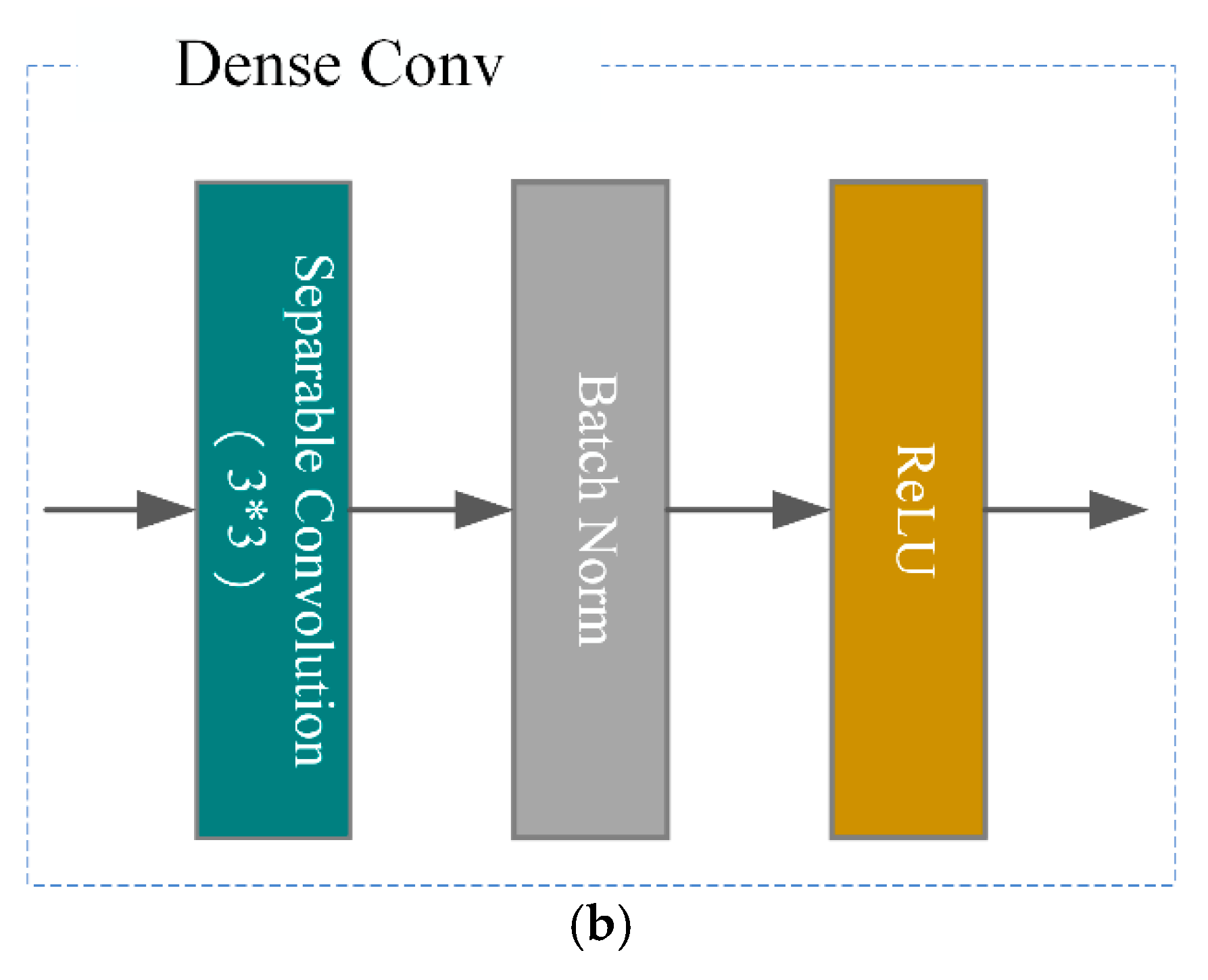
2.2.1. DenseNet
2.2.2. SAM and CAM
2.2.3. ASPP
2.3. CRFs
2.4. Accuracy Evaluation
3. Experiments and Results
3.1. Experimental Data
3.2. Experimental Results and Analysis
3.2.1. Visual Analysis of Classification Results
3.2.2. Analysis of the Accuracy of Classification Results
3.2.3. Analysis of Model Performance Differences before and after Optimization Using CRFs
3.3. Time Consumption
4. Discussion
5. Conclusions
Author Contributions
Funding
Institutional Review Board Statement
Informed Consent Statement
Data Availability Statement
Acknowledgments
Conflicts of Interest
Abbreviations
| CRFs | conditional random fields |
| DADNet | dual attention dense network |
| N-cut | normalized cut |
| FCN | fully convolutional network |
| ResNet | residual convolutional network |
| DenseNet | dense convolutional network |
| DANet | dual attention network |
| STDCNN | semi-transfer deep convolutional neural network |
| ASPP | atrous spatial pyramid pooling |
| SAM | spatial attention module |
| CAM | channel attention module |
| CBAM | convolutional block attention module |
| OA | overall accuracy |
| MIoU | mean intersection over union |
| LULC | land use/land cover |
| BiSeNet | bilateral segmentation network |
| A2-FPN | attention aggregation feature pyramid network |
| HED | holistically nested edge detection |
| GCN | graph convolutional network |
References
- Liu, X.; He, J.; Yao, Y.; Zhang, J.; Liang, H.; Wang, H.; Hong, Y. Classifying Urban Land Use by Integrating Remote Sensing and Social Media Data. Int. J. Geogr. Inf. Sci. 2017, 31, 1675–1696. [Google Scholar] [CrossRef]
- Hashem, N.; Balakrishnan, P. Change Analysis of Land Use/Land Cover and Modelling Urban Growth in Greater Doha, Qatar. Ann. GIS 2015, 21, 233–247. [Google Scholar] [CrossRef]
- Nguyen, K.-A.; Liou, Y.-A. Mapping Global Eco-Environment Vulnerability Due to Human and Nature Disturbances. MethodsX 2019, 6, 862–875. [Google Scholar] [CrossRef] [PubMed]
- Nguyen, K.-A.; Liou, Y.-A. Global Mapping of Eco-Environmental Vulnerability from Human and Nature Disturbances. Sci. Total Environ. 2019, 664, 995–1004. [Google Scholar] [CrossRef] [PubMed]
- Zhang, C.; Sargent, I.; Pan, X.; Li, H.; Gardiner, A.; Hare, J.; Atkinson, P.M. Joint Deep Learning for Land Cover and Land Use Classification. Remote Sens. Environ. 2019, 221, 173–187. [Google Scholar] [CrossRef] [Green Version]
- Patino, J.E.; Duque, J.C. A Review of Regional Science Applications of Satellite Remote Sensing in Urban Settings. Comput. Environ. Urban Syst. 2013, 37, 1–17. [Google Scholar] [CrossRef]
- Cassidy, L.; Binford, M.; Southworth, J.; Barnes, G. Social and Ecological Factors and Land-Use Land-Cover Diversity in Two Provinces in Southeast Asia. J. Land Use Sci. 2010, 5, 277–306. [Google Scholar] [CrossRef]
- Bing, Z. Current Status and Future Prospects of Remote Sensing. Bull. Chin. Acad. Sci. Chin. Version 2017, 32, 774–784. [Google Scholar] [CrossRef]
- Li-wen, H. The Cluster Analysis Approaches Based on Geometric Probability and Its Application in the Classification of Remotely Sensed Images. J. Image Graph. 2007, 12, 633–640. [Google Scholar] [CrossRef]
- Tehrany, M.S.; Pradhan, B.; Jebuv, M.N. A Comparative Assessment between Object and Pixel-Based Classification Approaches for Land Use/Land Cover Mapping Using SPOT 5 Imagery. Geocarto Int. 2014, 29, 351–369. [Google Scholar] [CrossRef]
- Halder, A.; Ghosh, A.; Ghosh, S. Supervised and Unsupervised Landuse Map Generation from Remotely Sensed Images Using Ant Based Systems. Appl. Soft Comput. 2011, 11, 5770–5781. [Google Scholar] [CrossRef]
- Adam, E.; Mutanga, O.; Odindi, J.; Abdel-Rahman, E.M. Land-Use/Cover Classification in a Heterogeneous Coastal Landscape Using RapidEye Imagery: Evaluating the Performance of Random Forest and Support Vector Machines Classifiers. Int. J. Remote Sens. 2014, 35, 3440–3458. [Google Scholar] [CrossRef]
- Maxwell, A.E.; Warner, T.A.; Fang, F. Implementation of Machine-Learning Classification in Remote Sensing: An Applied Review. Int. J. Remote Sens. 2018, 39, 2784–2817. [Google Scholar] [CrossRef] [Green Version]
- Hengkai, L.; Jiao, W.; Xiuli, W. Object Oriented Land Use Classification of Dongjiang River Basin Based on GF-1 Image. Trans. Chin. Soc. Agric. Eng. 2018, 34, 245–252. [Google Scholar] [CrossRef]
- Talukdar, S.; Singha, P.; Mahato, S.; Shahfahad, P.S.; Liou, Y.-A.; Rahman, A. Land-Use Land-Cover Classification by Machine Learning Classifiers for Satellite Observations—A Review. Remote Sens. 2020, 12, 1135. [Google Scholar] [CrossRef] [Green Version]
- Abdi, A.M. Land Cover and Land Use Classification Performance of Machine Learning Algorithms in a Boreal Landscape Using Sentinel-2 Data. GIScience Remote Sens. 2020, 57, 1–20. [Google Scholar] [CrossRef] [Green Version]
- Wang, H.; Qin, F.; Xu, C.; Li, B.; Guo, L.; Wang, Z. Evaluating the Suitability of Urban Development Land with a Geodetector. Ecol. Indic. 2021, 123, 107339. [Google Scholar] [CrossRef]
- Shapiro, L.G.; Stockman, G.C. Computer Vision; Prentice Hall: Hoboken, NJ, USA, 2001; ISBN 978-0-13-030796-5. [Google Scholar]
- Liang, X.; Luo, C.; Quan, J.; Xiao, K.; Gao, W. Research on Progress of Image Semantic Segmentation Based on Deep Learning. Comput. Eng. Appl. 2020, 56, 18–28. [Google Scholar] [CrossRef]
- Shi, J.; Malik, J. Normalized Cuts and Image Segmentation. IEEE Trans. Pattern Anal. Mach. Intell. 2000, 22, 888–905. [Google Scholar] [CrossRef] [Green Version]
- Rother, C.; Kolmogorov, V.; Blake, A. “GrabCut”: Interactive Foreground Extraction Using Iterated Graph Cuts. ACM Trans. Graph. 2004, 23, 309–314. [Google Scholar] [CrossRef]
- Deng, L. Deep Learning: Methods and Applications. FNT Signal Process. 2014, 7, 197–387. [Google Scholar] [CrossRef] [Green Version]
- Shelhamer, E.; Long, J.; Darrell, T. Fully Convolutional Networks for Semantic Segmentation. IEEE Trans. Pattern Anal. Mach. Intell. 2017, 39, 640–651. [Google Scholar] [CrossRef]
- He, K.; Zhang, X.; Ren, S.; Sun, J. Deep Residual Learning for Image Recognition; IEEE: Piscataway Township, NJ, USA, 2016; pp. 770–778. [Google Scholar]
- Huang, G.; Liu, Z.; van der Maaten, L.; Weinberger, K.Q. Densely Connected Convolutional Networks; IEEE: Piscataway Township, NJ, USA, 2017; pp. 4700–4708. [Google Scholar]
- Fu, J.; Liu, J.; Tian, H.; Li, Y.; Bao, Y.; Fang, Z.; Lu, H. Dual Attention Network for Scene Segmentation. arXiv 2019, arXiv:1809.02983, 3146–3154. [Google Scholar]
- Sun, Y.; Zhang, X.; Xin, Q.; Huang, J. Developing a Multi-Filter Convolutional Neural Network for Semantic Segmentation Using High-Resolution Aerial Imagery and LiDAR Data. ISPRS J. Photogramm. Remote Sens. 2018, 143, 3–14. [Google Scholar] [CrossRef]
- Wang, X.; Zhang, X.; Su, C. Land use classification of remote sensing images based on multi-scale learning and deep convolution neural network. J. ZheJiang Univ. Sci. Ed. 2020, 47, 715–723. [Google Scholar] [CrossRef]
- Huang, B.; Zhao, B.; Song, Y. Urban Land-Use Mapping Using a Deep Convolutional Neural Network with High Spatial Resolution Multispectral Remote Sensing Imagery. Remote Sens. Environ. 2018, 214, 73–86. [Google Scholar] [CrossRef]
- Ronneberger, O.; Fischer, P.; Brox, T. U-Net: Convolutional Networks for Biomedical Image Segmentation. In Proceedings of the Medical Image Computing and Computer-Assisted Intervention – MICCAI 2015; Navab, N., Hornegger, J., Wells, W.M., Frangi, A.F., Eds.; Springer International Publishing: Cham, Switzerland, 2015; pp. 234–241. [Google Scholar]
- Chen, L.-C.; Papandreou, G.; Kokkinos, I.; Murphy, K.; Yuille, A.L. DeepLab: Semantic Image Segmentation with Deep Convolutional Nets, Atrous Convolution, and Fully Connected CRFs. IEEE Trans. Pattern Anal. Mach. Intell. 2018, 40, 834–848. [Google Scholar] [CrossRef] [Green Version]
- Woo, S.; Park, J.; Lee, J.-Y.; Kweon, I.S. CBAM: Convolutional Block Attention Module. In Computer Vision—ECCV 2018; Ferrari, V., Hebert, M., Sminchisescu, C., Weiss, Y., Eds.; Lecture Notes in Computer Science; Springer International Publishing: Cham, Switzerland, 2018; Volume 11211, pp. 3–19. ISBN 978-3-030-01233-5. [Google Scholar]
- Liu, R.; Shen, J.; Wang, H.; Chen, C.; Cheung, S.; Asari, V.K. Enhanced 3D Human Pose Estimation from Videos by Using Attention-Based Neural Network with Dilated Convolutions. Int. J. Comput. Vis. 2021, 129, 1596–1615. [Google Scholar] [CrossRef]
- Lafferty, J.D.; McCallum, A.; Pereira, F.C.N. Conditional Random Fields: Probabilistic Models for Segmenting and Labeling Sequence Data. In Proceedings of the Eighteenth International Conference on Machine Learning; Morgan Kaufmann Publishers Inc.: San Francisco, CA, USA, 2001; pp. 282–289. [Google Scholar]
- Krähenbühl, P.; Koltun, V. Efficient Inference in Fully Connected CRFs with Gaussian Edge Potentials. In Proceedings of the Advances in Neural Information Processing Systems; Curran Associates Inc.: Red Hook, NY, USA, 2011; Volume 24. [Google Scholar]
- Xiao, C.; Li, Y.; Zhang, H.; Chen, J. Semantic segmentation of remote sensing image based on deep fusion networks and conditional random field. Zggx 2021, 24, 254–264. [Google Scholar] [CrossRef]
- Tong, X.-Y.; Xia, G.-S.; Lu, Q.; Shen, H.; Li, S.; You, S.; Zhang, L. Land-Cover Classification with High-Resolution Remote Sensing Images Using Transferable Deep Models. Remote Sens. Environ. 2020, 237, 111322. [Google Scholar] [CrossRef] [Green Version]
- Yu, C.; Wang, J.; Peng, C.; Gao, C.; Yu, G.; Sang, N. BiSeNet: Bilateral Segmentation Network for Real-Time Semantic Segmentation. arXiv 2018, arXiv:1808.00897, 325–341. [Google Scholar]
- Hou, B.; Liu, Y.; Rong, T.; Ren, B.; Xiang, Z.; Zhang, X.; Wang, S. Panchromatic Image Land Cover Classification Via DCNN with Updating Iteration Strategy. In Proceedings of the IGARSS 2020–2020 IEEE International Geoscience and Remote Sensing Symposium, 2 October–26 September 2020; pp. 1472–1475. [Google Scholar]
- Li, R.; Wang, L.; Zhang, C.; Duan, C.; Zheng, S. A2-FPN for Semantic Segmentation of Fine-Resolution Remotely Sensed Images. Int. J. Remote Sens. 2022, 43, 1131–1155. [Google Scholar] [CrossRef]
- He, C.; Li, S.; Xiong, D.; Fang, P.; Liao, M. Remote Sensing Image Semantic Segmentation Based on Edge Information Guidance. Remote Sens. 2020, 12, 1501. [Google Scholar] [CrossRef]
- He, S.; Lu, X.; Gu, J.; Tang, H.; Yu, Q.; Liu, K.; Ding, H.; Chang, C.; Wang, N. RSI-Net: Two-Stream Deep Neural Network for Remote Sensing Images-Based Semantic Segmentation. IEEE Access 2022, 10, 34858–34871. [Google Scholar] [CrossRef]
- Li, J.; Xiu, J.; Yang, Z.; Liu, C. Dual Path Attention Net for Remote Sensing Semantic Image Segmentation. ISPRS Int. J. Geo-Inf. 2020, 9, 571. [Google Scholar] [CrossRef]
- Yang, K.; Liu, Z.; Lu, Q.; Xia, G.-S. Multi-Scale Weighted Branch Network for Remote Sensing Image Classification; IEEE: Piscataway Township, NJ, USA, 2019; pp. 1–10. [Google Scholar]


| Payload | Bands | Band Range (µm) | Spatial Resolution(m) | Width (km) | Side-Swing Capability | Orbital Period (Day) |
|---|---|---|---|---|---|---|
| Panchromatic multispectral camera | 1 | 0.45–0.90 | 1 | 45 | ±35° | 5 |
| 2 | 0.45–0.52 | 4 | ||||
| 3 | 0.52–0.59 | |||||
| 4 | 0.63–0.69 | |||||
| 5 | 0.77–0.89 |
| Built-Up | Farmland | Forest | Water | Meadow | Background | |
|---|---|---|---|---|---|---|
| Train | 6.19 × 10⁸ | 1.71 × 10⁹ | 1.85 × 10⁸ | 5.92 × 10⁸ | 1.37 × 10⁸ | 2.63 × 10⁹ |
| Validation | 8.70 × 10⁷ | 2.54 × 10⁸ | 1.79 × 10⁷ | 9.97 × 10⁷ | 5.74 × 10⁴ | 2.76 × 10⁸ |
| Test | 5.38 × 10⁷ | 2.55 × 10⁸ | 7.10 × 10⁷ | 8.80 × 10⁷ | 7.70 × 10⁶ | 2.59 × 10⁸ |
| Total Percentage | 10.72% | 31.37% | 3.87% | 11.01% | 2.05% | 40.98% |
| Model | Category | Recall | Precision | F1-Score | OA | MIoU | Kappa |
|---|---|---|---|---|---|---|---|
| FCN-8s | built-up | 83.38% | 71.08% | 76.74% | 80.62% | 57.52% | 75.35% |
| farmland | 75.33% | 87.02% | 80.75% | ||||
| forest | 82.33% | 88.17% | 85.15% | ||||
| water | 88.49% | 85.70% | 87.07% | ||||
| meadow | 75.32% | 40.14% | 52.37% | ||||
| BiSeNet | built-up | 85.20% | 72.56% | 78.37% | 86.37% | 67.66% | 82.63% |
| farmland | 83.00% | 85.89% | 84.42% | ||||
| forest | 90.43% | 85.42% | 87.85% | ||||
| water | 90.16% | 90.93% | 90.54% | ||||
| meadow | 76.00% | 44.67% | 56.27% | ||||
| DADNet-CRFs | built-up | 87.72% | 74.18% | 80.38% | 87.98% | 69.47% | 84.70% |
| farmland | 85.32% | 88.11% | 86.69% | ||||
| forest | 90.89% | 86.62% | 88.70% | ||||
| water | 92.17% | 87.85% | 89.96% | ||||
| meadow | 79.37% | 47.40% | 59.36% |
| Method | Built-Up | Farmland | Forest | Water | Meadow | OA |
|---|---|---|---|---|---|---|
| FCN-8s | 88.29% | 67.63% | 80.02% | 96.59% | 0.00% | 90.00% |
| FCN-8s-CRFs | 89.24% | 69.01% | 82.14% | 96.60% | 0.00% | 90.70% |
| BiSeNet | 89.65% | 64.17% | 87.44% | 96.64% | 0.00% | 91.21% |
| BiSeNet-CRFs | 91.50% | 67.81% | 89.16% | 96.84% | 0.00% | 92.44% |
| DADNet | 92.44% | 60.90% | 88.03% | 97.25% | 0.00% | 92.62% |
| DADNet-CRFs | 93.09% | 61.02% | 89.16% | 97.30% | 0.00% | 93.04% |
| Method | DADNet-CRFs | FCN-8s | BiSeNet |
|---|---|---|---|
| time(s) | 3158.00 | 4285.00 | 3288.00 |
| average time(s) | 45.11 | 61.21 | 46.97 |
Publisher’s Note: MDPI stays neutral with regard to jurisdictional claims in published maps and institutional affiliations. |
© 2022 by the authors. Licensee MDPI, Basel, Switzerland. This article is an open access article distributed under the terms and conditions of the Creative Commons Attribution (CC BY) license (https://creativecommons.org/licenses/by/4.0/).
Share and Cite
Zheng, K.; Wang, H.; Qin, F.; Han, Z. A Land Use Classification Model Based on Conditional Random Fields and Attention Mechanism Convolutional Networks. Remote Sens. 2022, 14, 2688. https://doi.org/10.3390/rs14112688
Zheng K, Wang H, Qin F, Han Z. A Land Use Classification Model Based on Conditional Random Fields and Attention Mechanism Convolutional Networks. Remote Sensing. 2022; 14(11):2688. https://doi.org/10.3390/rs14112688
Chicago/Turabian StyleZheng, Kang, Haiying Wang, Fen Qin, and Zhigang Han. 2022. "A Land Use Classification Model Based on Conditional Random Fields and Attention Mechanism Convolutional Networks" Remote Sensing 14, no. 11: 2688. https://doi.org/10.3390/rs14112688