Abstract
Based on marine environmental factors of different sea areas, a high-performance sea clutter time series modeling algorithm for the real sea surface is developed to study the amplitude mean and Doppler spectrum characteristics of sea clutter. The European Centre for Medium-Range Weather Forecasts (ECMWF) data set (ERA-Interim) and ESA’s soil moisture and ocean salinity (SMOS) data set are utilized to establish databases of different marine environmental factors. Combined with the mixed spectrum model, the geometric fine structure of wind-driven sea surface with swell superposition is established by using the double-superposition method (DSM) and comprehensively considering small-scale capillary ripples, large-scale gravity waves and swell. A triangle facet-based sea clutter series modeling algorithm is developed, in which the quasi-specular scattering based on a triangle and the scattering based on gravity wave modulation capillary spectrum are calculated, respectively, and compared with the measured results. For high-resolution radar, dynamic sea surface modeling and sea clutter calculation are very time consuming. In this paper, the Tesla K80 GPU manufactured by NVIDIA in Santa Clara, Computed Unified Device architecture (CUDA) high-performance parallel technology and some optimization strategies are adopted to improve the efficiency of sea clutter modeling. The results can be used to analyze the distribution characteristics of marine factors, the average amplitude and Doppler characteristics of sea clutter in different sea areas.
1. Introduction
The characteristics of sea clutter in real marine environments of different sea areas are of great significance in the application fields of radar detection, remote sensing, SAR imaging and situation awareness [1,2,3,4]. China’s coastal waters are vast, with great differences in latitude, geographical location and environmental distribution. It is close to the Bohai Sea, the Yellow Sea, the East China Sea and the South China Sea. Among them, the Bohai Sea belongs to the inland sea, and the characteristics of wind and waves are relatively gentle due to the influence of surrounding land and wind; the South Sea and the Western Pacific are deep-sea areas, which are greatly affected by wind speed and ocean dynamics. Different sea areas are affected by geographical environment and differences in marine environmental parameters, resulting in different scattering mechanisms in different sea areas. The traditional research on electromagnetic scattering characteristics of sea surface is generally based on the fully developed theoretical model of wind wave spectrum [5,6,7,8,9]. A superposition method based on wind wave spectrum is proposed for high-performance sea surface modeling [5]. Wu [6] optimized the traditional two-scale method to analyze the scattering coefficient characteristics of sea surface with high sea situation. The small-slope approximation [7,8,9] is utilized to study the Doppler spectrum of nonlinear sea surface electromagnetic scattering. However, the above parameters are generally wind speed and wind direction, which are not consistent with the actual sea surface state. The information in the backscattered echo cannot reflect the real state of the sea surface, such as wave height and wave period.
The actual sea surface is composed of wind waves and swells, and the wavelength is usually in the range of a few centimeters to hundreds of meters; wind waves are generated in the local wind area, so they are strongly coupled with the local wind field. On the contrary, swells are usually caused by distant storms and can travel thousands of kilometers over the sea. Drennan’s research [10] found that the pure wind wave sea surface state often occurs in coastal areas, closed sea areas and extreme wind field events, while in open sea areas, swell often exists with wind waves. Edso found that [11] the wave phase velocity usually exceeds the wind speed by studying data from the North Atlantic, which also confirmed the existence of swell.
The instantaneous scattered electromagnetic field on the sea surface can generate the original synthetic aperture radar data profile in the real marine environment, which can obtain more detailed motion information of the surface micro rough surface and Doppler characteristics. A large number of scholars [12,13,14,15,16] calculate the sea surface scattering field based on the facet approximation method proposed by Clarizia [17]. However, some [12,13] can only calculate the scattering coefficient and cannot obtain the instantaneous scattering field; some [13,14] only consider Bragg scattering, which will produce wrong results when the incident is at a small angle; and some [15,16] do not consider the actual marine environmental factors, such as wave height and wave period.
In the traditional time-varying sea EM scattering calculation process, a single sea surface will produce a large number of bins according to the calculation accuracy requirements, which will make the real sea clutter time series very time consuming. Some scholars use GPU and NVIDIA’s CUDA high-performance parallel technology to speed up. In [5], CUDA parallel computing is used to simulate large-scale dynamic sea surface, and nearly 800× speedup is obtained. Su [18] used parallel technology to significantly improve the efficiency of EM scattering calculation of double-layer vegetation. Wu [15] proposed a facet-based parallel scattering field algorithm, which combined with five optimization strategies to make sea clutter calculation possible. CUDA parallel technology can also be applied to an image autoregressive interpolation model [19] and obtain good results.
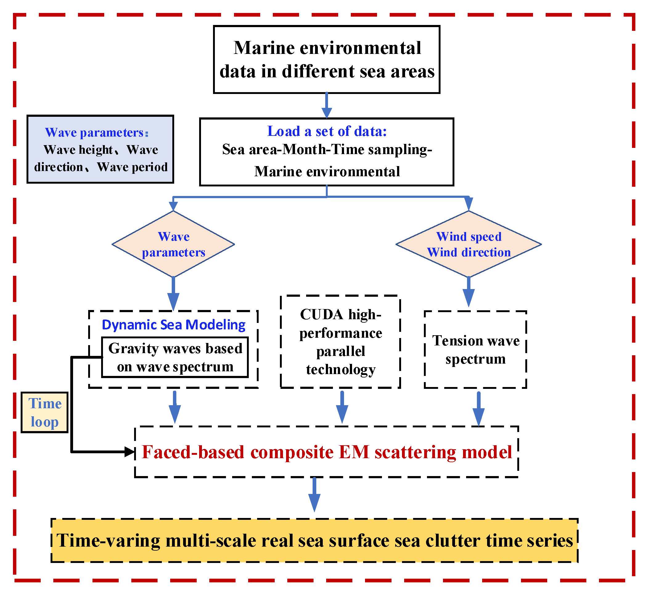
In this paper, based on the European Centre for Medium-Range Weather Forecasts (ECMWF) data set (ERA-Interim) [20] and ESA’s soil moisture and ocean salinity (SMOS) data set [21], the data sets of marine environmental factors in different sea areas of China are established. The gravity wave is generated according to the wave height, wave period and wave direction; the small-scale sea surface is superimposed according to the slope of large-scale gravity wave, so as to generate a real sea surface model, considering different marine environmental factors. Finally, combined with CUDA parallel technology, a high-performance sea clutter modeling algorithm is proposed to analyze the EM scattering characteristics of real sea surface in different sea areas.
The reminder of this paper is organized as follows: Section 2 simulates the real dynamic sea surface based on the mixed sea spectrum. Section 3 establishes the sea clutter time series by using the facet-based composite EM scattering parallel algorithm. Section 4 analyzes the amplitude and Doppler characteristics of sea clutter. Section 5 gives the conclusions and prospects.
2. Real Dynamic Sea Surface Simulation
Actual sea waves are complex and changeable. For the application of marine engineering, although the marine experiment is more intuitive, it is limited by geographical location, as well as being time consuming and laborious. The geometric modeling of sea surface based on wave spectrum is an important and basic method to study the interaction mechanism between EM waves and sea surface. In fact, to realize large-scale sea surface geometric modeling based on a wave spectrum model, it is important to consider the long wave component of the wave spectrum. For the problem of sea surface EM scattering, small-scale capillary ripples are more important characteristic information, so the modulation effect of gravity waves needs to be considered. Using the linear superposition method, the small-scale ripples are superimposed according to the slope distribution of large-scale gravity waves.
2.1. Factors of Marine Environment
The original meteorological satellite data cover the whole world. This paper selects the ECMWF data set (ERA-Interim) from January 2015 to December 2017. The longitude range is and . The resolution grid of satellite data is , the daily sampling interval of data is 6 h, and each marine environmental element constitutes a data matrix at each sampling time every day. The database can directly obtain the wind speed, wave height , average wave period , wave direction , temperature and other marine environmental parameters 10 m above the sea surface. In the directly obtained data, the wind speed is divided into two components: radial part and zonal part , which must be converted into the same wind speed and direction . In order to make the wind speed direction consistent with the wave direction, the wave direction needs to be converted.
Figure 1 compares the relationship between wave direction and wind direction before and after the conversion during the continuous sampling period in the Yellow Sea in October 2014. The sampling interval is 6 h. As Figure 1 shows, the converted wave direction has a high correlation with the wind direction, which is more in line with the actual situation.
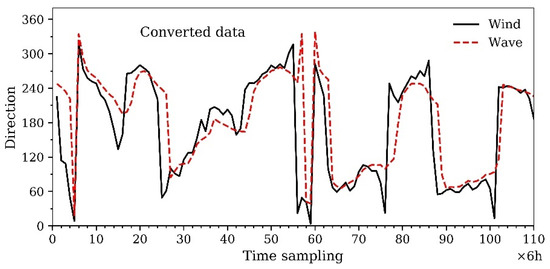
Figure 1.
Comparison between converted wave direction and wind direction in the Yellow Sea.
The ERA-Interim is utilized in this paper to establish the marine environment database, but the database does not include marine salinity data. In order to make up for this deficiency, the salinity data of different sea areas in China are obtained through ESA SMOS.
2.2. Hybrid Wave Spectrum Model of Real Sea Surface
The formation of actual sea surface waves is affected by the interaction of wind, gravity and surface tension. Generally, the energy distribution characteristics of real sea waves are represented by the wave energy spectrum distribution function . For the real sea surface, the energy spectrum is also related to the direction , so the actual sea surface energy spectrum is two-dimensional, which can be expressed as:
where, is the distribution characteristics of wave energy in different directions and refers to the direction of the wave relative to the radar.
The actual sea surface usually contains two peaks generated by wind waves and swells. In this paper, the one-dimensional hybrid wave spectral function proposed by Torsethaugen and Haver [22] is used:
where, subscript corresponds to the main wave and secondary wave, respectively and and represent the wave height and wave period, respectively; , , is the spatial frequency of sea waves; , .
The hybrid wave spectrum consists of two parts: wind wave and swell. The periodic condition of fully developed sea surface is introduced to distinguish the proportion of the superposition of two wave forms. Factor is a constant related to the range of wind area. When the wind area is equal to 370 square kilometers, . When , the hybrid wave is dominated by wind wave; when , the hybrid wave is dominated by swell. The detailed definition of relevant variables in Table 1 are as follows:
where, , , , , , , , , , , .

Table 1.
Parameter calculation formula under different waveforms.
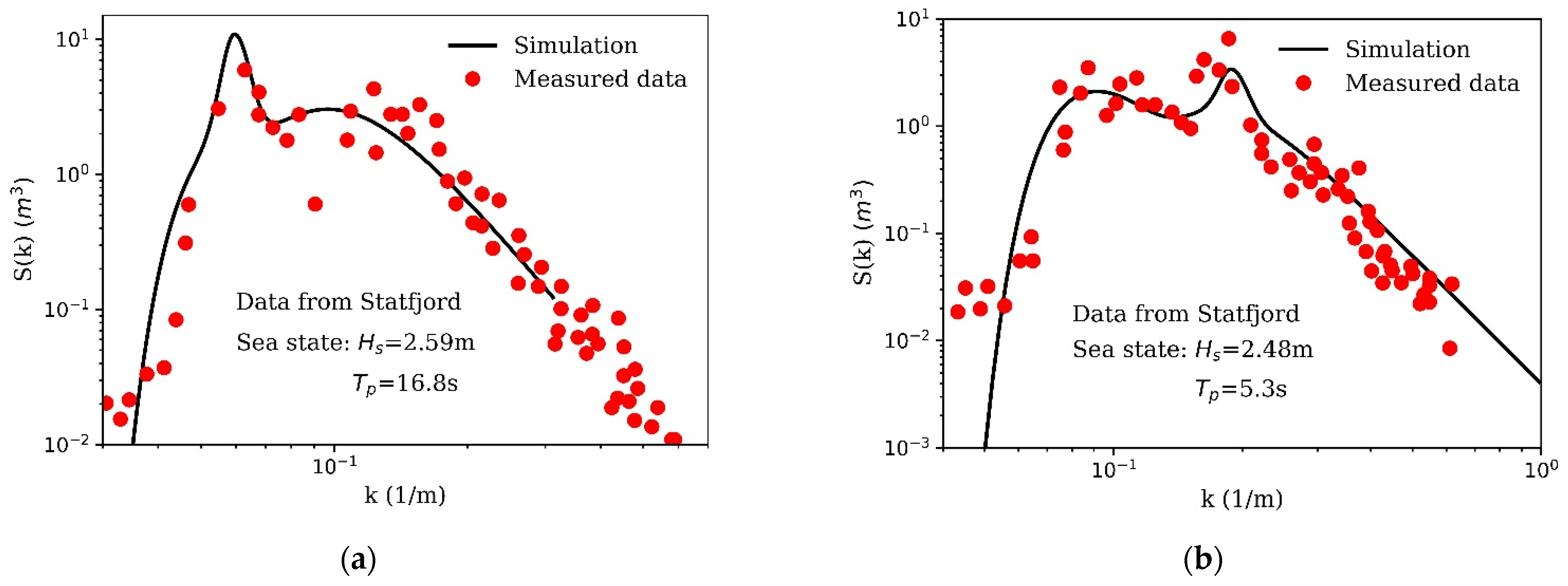
Figure 2 shows the variation law of hybrid wave energy spectrum with frequency under swell-dominated and wind-wave-dominated conditions, and compares it with the measured data [22]. It can be clearly seen in Figure 2 that both the hybrid sea spectrum model and the measured wave spectrum show a bimodal phenomenon, which is more in line with the actual sea surface characteristics.
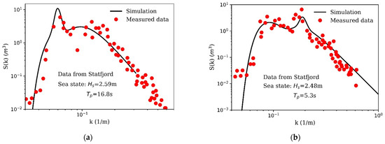
Figure 2.
Comparison of hybrid sea spectrum with measured data. (a) Dominated by swells. (b) Dominated by wind waves.
The directional spectrum in Equation (1) is cos-2s [23] direction spectrum:
where, is the wave direction, is the average wave direction, is the diffusion function, which is the empirical value controlling the wave propagation around the average wave direction, and is the gamma function. The parameters , , and are constants related to the characteristics of ocean waves. When the sea wave is dominated by wind waves, , , . When the sea wave is dominated by swells, , , . represents the corresponding frequency at the wave crest [23].
2.3. Real Dynamic Sea Surface Simulation
For the time-varying sea surface, the height at a certain time can be approximately the superposition of the cosine waves. According to the linear superposition method [24], the height of the sea surface can be expressed as:
where, is the hybrid spectrum model based on the marine environmental elements and the initial phase satisfies the uniform distribution between . , , and correspond to the wave number, circular frequency and direction angle. The constants M and N are the sampling points on the frequency and direction angle, respectively.
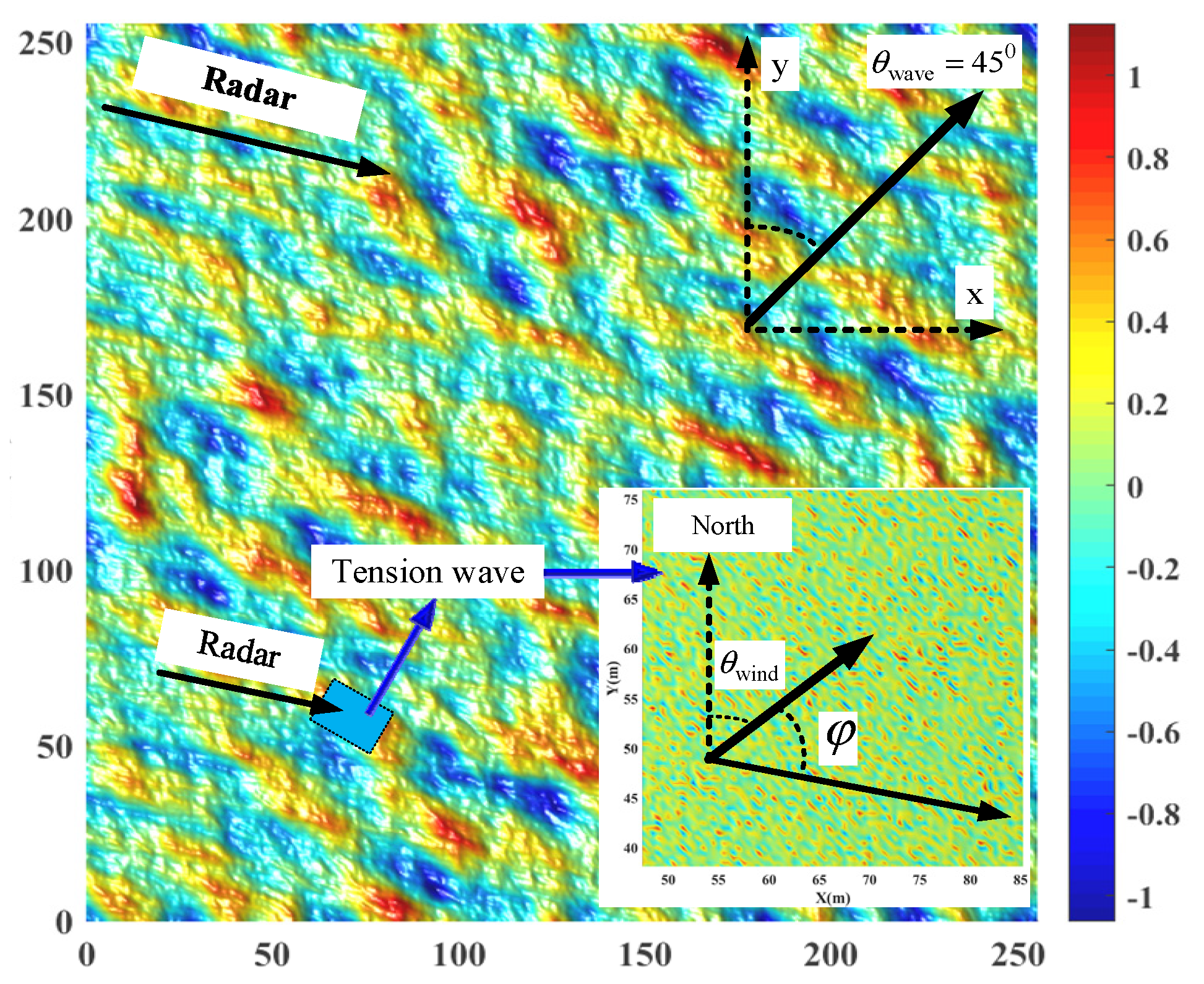
The gravity wave is directly reflected in wave height, wave period and wave direction, which can be simulated by using the marine environment elements according to the hybrid sea surface. The small-scale tension waves are superimposed according to the slope distribution of the large-scale gravity wave by linear superposition. The sea surface height can finally be expressed as:
where, is the position vector, represents the position vector of each facet on the gravity waves, represents the position vector corresponding to tensile waves. and are the slope of the gravity wave along the x and y directions, respectively. is gravity wave and is the tensile wave superimposed on it. In general, the resolution accuracy of the gravity wave is rough, while the tension wave needs high-precision segmentation. Therefore, when generating superimposed waves, the gravity wave needs to be further segmented according to the accuracy of the tension wave.
3. High-Performance Computing of Sea Clutter
The real ocean surface is divided into two parts by the linear superposition method: gravity wave and capillary tension wave. Figure 3 shows the EM scattering diagram of the sea surface illuminated by radar. When the incident angle is less than 20 degrees, the quasi-specular scattering mechanism caused by large-scale gravity waves plays a leading role; when the incident angle is 20~70 degrees, the Bragg scattering mechanism caused by the capillary tension wave plays a leading role. When the incident angle is greater than 70 degrees, the Bragg scattering mechanism still exists, but the wave breaking, foam coverage and multiple scattering effects will affect the EM scattering characteristic of the sea surface.
Figure 3.
EM scattering mechanism of radar-illuminated sea surface.
3.1. Sea Clutter Calculation of Large-Scale Gravity Waves
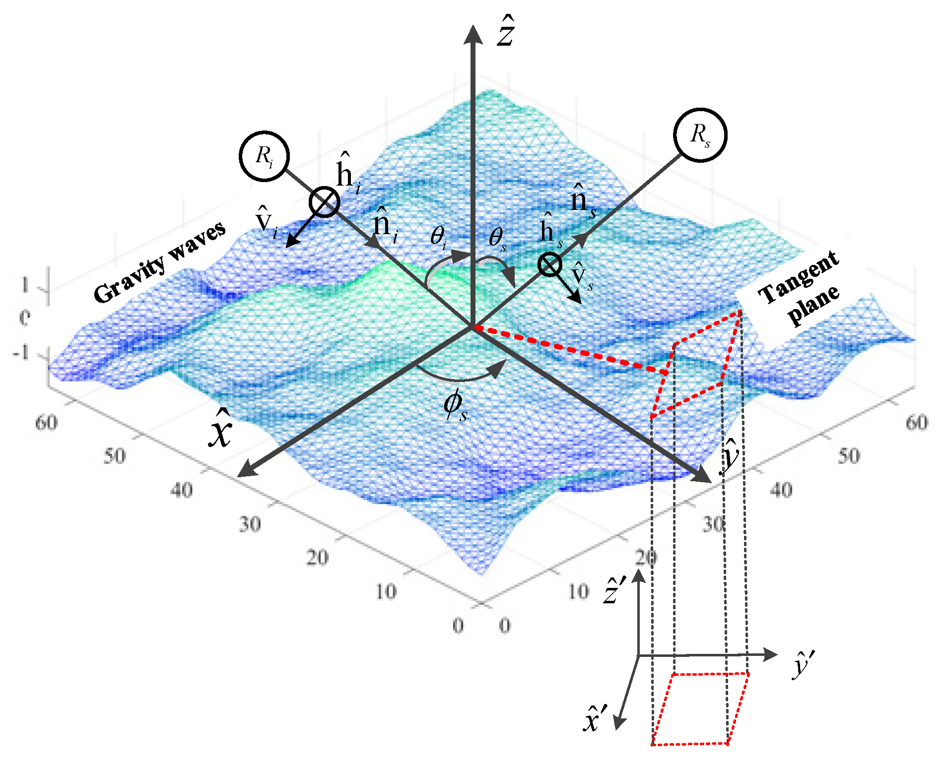
Large-scale gravity wave scattering is shown in Figure 4. When the local radius of the curvature is much larger than the incident wavelength, the Kichhoff approximation [25] method can solve the Stratton–Chu integral equation [26]. In this case, the sea surface facet can be approximated as a smooth facet.
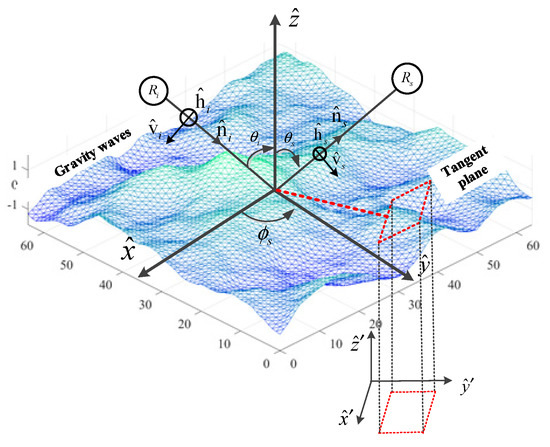
Figure 4.
Quasi-specular scattering mechanisms for large-scale gravity waves.
The incident field can be expressed as:
where, is the incident wave number, is the distance from the wave source to the center of the irradiation area, is the unit polarization vector and represents the unit vector in the incident direction.
The scattering field under Kirchhoff approximation [25] can be written as:
where,
where, represents the unit normal vector of local panel, is the scattering wave number, represents the distance from the observation point to the center of the irradiation area. For sea surface EM scattering, , and corresponds to radar wavelength and is the center coordinate of each calculation facet of the sea surface.
Substituting Equations (19) and (20) into Equation (18), we can obtain:
where, represents the polarization factor of different polarization, which is a function of incident angle, scattering angle and Fresnel reflection coefficient [25], , , and represent the sampling steps of gravity waves in the x and y directions.
3.2. Sea Clutter Calculation of Tension Waves
Different wind speeds and directions produce instantaneous capillary waves, which are superimposed on the sea surface of gravity waves. When the radar irradiates the capillary wave, only the capillary wave component meeting the resonance condition can cause Bragg scattering, which can be expressed as:
where, is the position coordinate vector of the capillary waves, is the wind direction. represents the amplitude of capillary wave, corresponds to the high wave vector in the sea wave spectrum, is the area of the facet, is the angular frequency, is the wave number of Bragg resonant capillary wave component, which can be expressed as:
where, , is the projection of in Equation (19) on the tension wave.
The small perturbation method (SPM) can well calculate the Bragg scattering field corresponding to capillary tension waves. According to the perturbation field expression [27] proposed by Fuks, the scattering field can be expressed as:
where, represents the incident wave and is the scattering amplitude matrix, expressed as:
where, is the electric constant, and is the polarization factor matrix of scattering amplitude, which is determined by incident angle, scattering angle, polarization and Fresnel reflection coefficient.
Small-scale tension waves are modulated by large-scale gravity waves. Considering the capillary wave is modulated by gravity wave, the polarization factor in the local coordinate system can be calculated as:
where, , , , and are the incident angle, incident azimuth and scattering azimuth in the local coordinate system. and are the Fresnel reflection coefficients of different polarizations, is the dielectric parameter of sea surface.
For a single facet, the integral term in Equation (26) can be written as:
According to the Euler formula and Bessel function, Equation (31) can be expressed as:
where, represents the first Bessel function of order n, represents the components of the normal vector along the z-axis,
By calculating the integral term in Equation (32), we can obtain:
3.3. Sea Clutter Simulation Based on Real Sea Surface
This paper comprehensively considers the quasi-specular scattering mechanism and Bragg scattering mechanism, and the scattering field corresponding to each scattering unit on the actual sea surface can be calculated. Assuming that each facet is statistically independent of one other, the calculation formula of the total electromagnetic scattering field of the actual sea surface is as follows:
where, is the quasi-specular scattering field, is the gravity-wave-modulated capillary wave scattering field. According to the cut off wave number , if , the scattering field can be calculated by ; on the contrary, the scattering field can be calculated by .
The core algorithm of this paper is based on the calculation of capillary wave sea clutter modulated by a gravity wave. Therefore, the sea surface subdivision accuracy is related to different frequency bands. Generally, the facet size is times of the Bragg wavelength. The real sea surface subdivision accuracy of different radar bands is shown in Table 2. Based on the real sea surface EM scattering field algorithm, combined with the time series sea surface considering the real marine environment elements, the sea clutter time series simulation results of given radar parameters under the corresponding marine environment parameters of different sea areas can be obtained.
Table 2.
Sea surface subdivision accuracy for different radar bands.
Figure 5 shows the modeling diagram of sea clutter time series considering the real marine environment elements. is the time and the time sampling interval is related to the radar frequency band. In Plant’s research [28], it is pointed out that the corresponding sampling interval for X and Ka bands should not be less than 0.01 s and 0.003 s, respectively. In this paper, the number of time series sampling n is 1024 times. Time sampling num is the number of effective marine environment sample groups in the selected sea area in the current month.
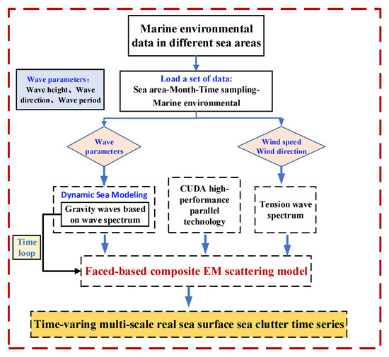
Figure 5.
Schematic diagram of sea clutter time series modeling of sea surface with marine environmental elements in different sea areas.
For each month, in any sea area, it is assumed that only 100 groups of marine environment samples are calculated. In fact, the number of sea surfaces to be calculated is 102,400. Considering the subdivision accuracy of each sea surface, taking Ku band as an example, the facet subdivision accuracy needs to be , so at least facets are required for calculation. It takes about 10 h to complete the sea clutter time series under a set of marine environmental elements. The simple application of traditional methods to calculate sea clutter time series is very time consuming and inefficient. It is difficult to simulate and model the sea surface on such a large number of marine environmental elements in different sea areas.
3.4. Parallel Computing of GPU-CPU Heterogeneous System Based on CUDA
CUDA is a general program language designed by NVIDIA. It can realize data transmission and operation between CPU and GPU through specific syntax and storage modes. A typical CUDA program generally consists of three parts: (1) copy the initial value from the host to the GPU device memory; (2) parallel execution of program functions on the device; (3) returns the calculation result to the host memory.
The time-varying sea clutter parallel modeling algorithm based on CUDA is adopted, and a large number of computing units are used to calculate the EM scattering of sea surface. The computing equipment is shown in Table 3.
Table 3.
Computing device platform configuration information.
Fine-grained data parallelism is the fundamental way for CUDA to realize parallel execution. A kernel function will create a grid. A grid is composed of three blocks of a three-dimensional array, and each thread block is a three-dimensional array composed of three-dimensional threads. The threads in each thread block will execute the kernel function in parallel. For parallel programs, data concurrency is very important. In this paper, the composition of thread blocks in each grid is , and the composition of threads in each thread block is . Finally, the kernel function is executed for calculation and the sea clutter time series is transmitted back to the CPU.
Figure 6 shows the results of CUDA-based parallel computing. For the marine environment is the South China Sea in September and October, the radar band is S-band, the sea surface range is , the subdivision accuracy is , the time interval is 0.005 s and the number of sea surfaces in the time series is 1024. As shown in the figure, it takes 661.76 s to process the sea clutter time series of 100 groups of sea clutter time series in September and 647.61 s for 100 groups in October, with a slight deviation. However, when the subdivision accuracy is selected as , it takes about 25 s to process a group of sea clutter time series, about four-times that of the former, indicating that the calculation time of the high-performance parallel computing algorithm is stable and makes full use of the computing potential of GPU. After adopting the high-performance algorithm, it can meet the requirements of large-scale operation, which makes it possible to establish the data set of sea clutter characteristics of marine environment elements in different sea areas.
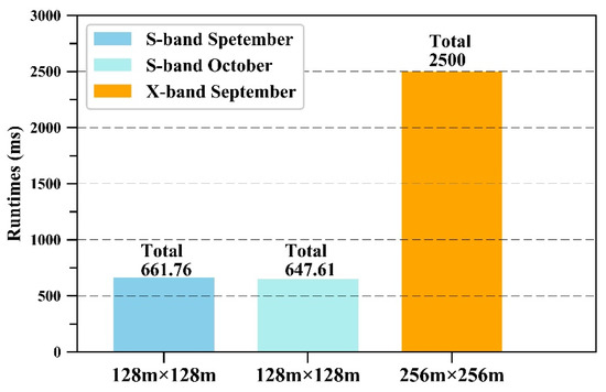
Figure 6.
Processing time (ms) of high-performance parallel programs on different sizes of sea surface.
4. Results
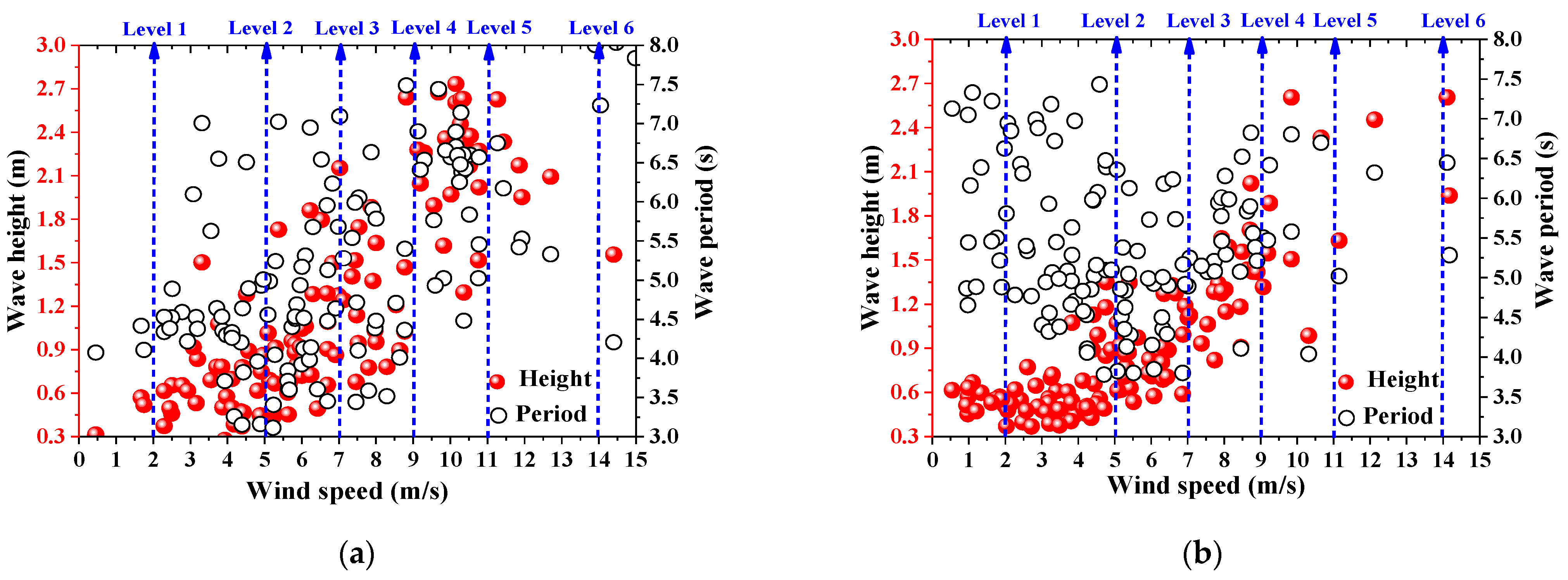
Real marine environment elements, such as wind speed, wind direction, wave height, wave direction and wave period, are not linear. Figure 7 shows the relationship between wind speed and wave period in winter (January) and summer (August) in the Yellow Sea. Referring to Douglas Sea state table, the wind speed corresponding to level 1–6 sea state is marked with a dotted line. As shown in Figure 7, the marine environmental elements of the Yellow Sea are basically below a level 5 sea state. For the same sea state, the distribution of wave height and wave period in January is discrete and the correlation between wave height and wind speed in August is strong, indicating the wave height, wave period and wind speed are not linear. Therefore, it is limited to simply use the traditional sea spectrum to describe the multi-scale sea surface and EM scattering characteristics.

Figure 7.
Relationship between wind speed, wave height and wave period in the Yellow Sea in January and August 2017. (a) January, (b) August.
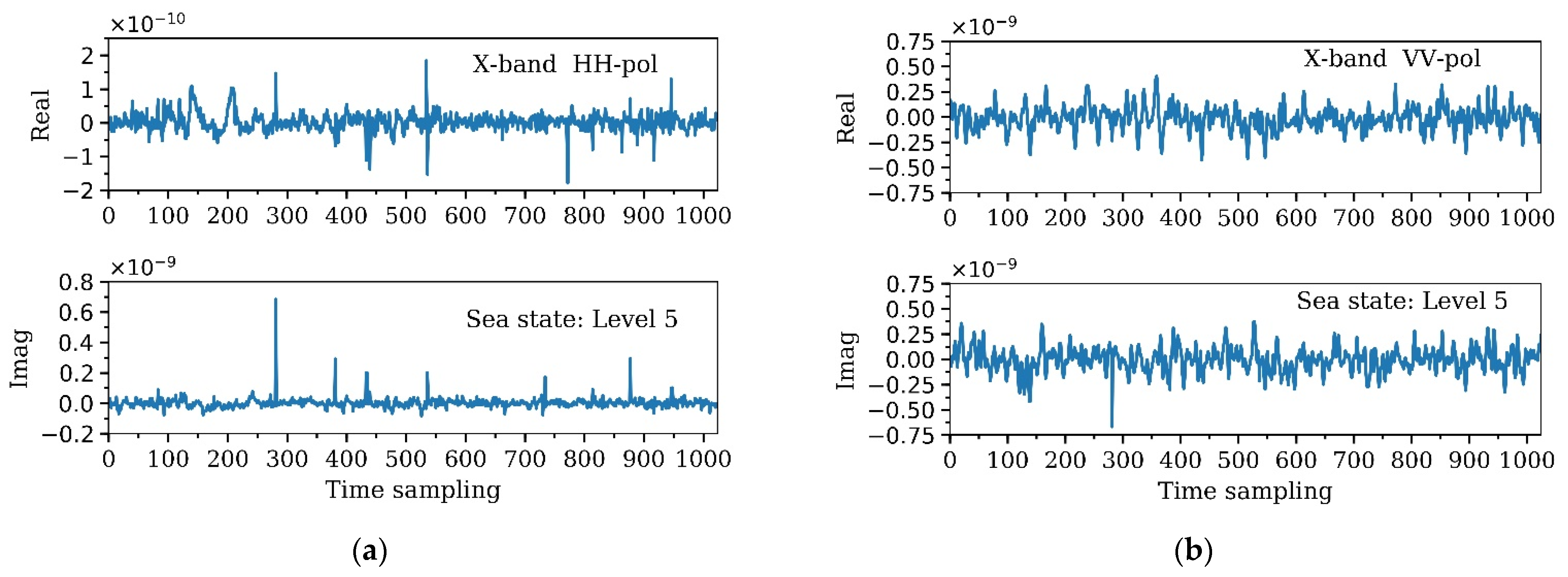
Figure 8 shows the calculation results of the corresponding mean values of the real and imaginary parts of the scattering fields of different polarizations in the Yellow Sea. The time sampling interval is set to 0.005 s, the sea surface size is set to and the subdivision accuracy is . The grazing angle is , wind speed is , wind direction is , wave height is , wave direction is and wave period is 5.02 s.
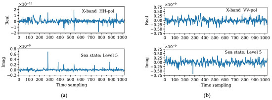
Figure 8.
Time series simulation results of sea clutter with different polarizations in X-band in the Yellow Sea. (a) HH polarization; (b) VV polarization.
4.1. Mean Amplitude Characteristics of Sea Clutter
According to the radar equation, the normalized radar cross section (NRCS) of multi-scale real sea surface can be expressed as:
where, is the sea surface scattering field calculated by Equation (37), represents the amplitude of the incident field and is the area of the sea surface.
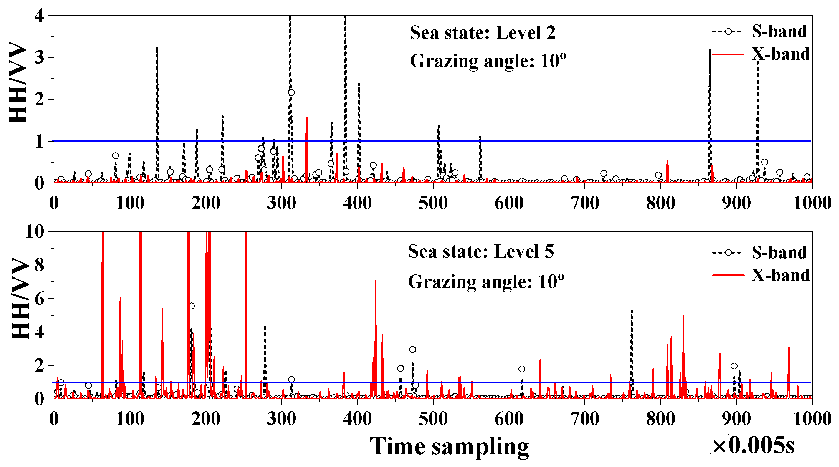
Figure 9 shows the amplitude mean polarization ratio of S-band and X-band scattering coefficients under different sea conditions. As shown in Figure 9, under level 2 sea state, in most cases, the amplitude mean polarization ratio of scattering coefficient is less than 1; that is, the scattering coefficient of HH polarization is less than that of VV polarization. With the increase in sea state and wave band, the situation of HH polarization being greater than VV polarization obviously increases. On the one hand, the mean value of VV polarization is smaller than that of the VV polarization. On the other hand, the change in rough sea surface can easily affect the scattering echo of HH polarization. According to the scattering mechanism of rough sea surface, the changes in sea surface and radar parameters have a stronger impact on HH polarization scattering echo. Therefore, under high sea states (level 5), the EM wave with shorter wavelength (X-band) is more likely to produce HH polarization echo larger than VV polarization echo.

Figure 9.
Amplitude mean polarization ratio of different bands under different sea conditions (HH/VV).
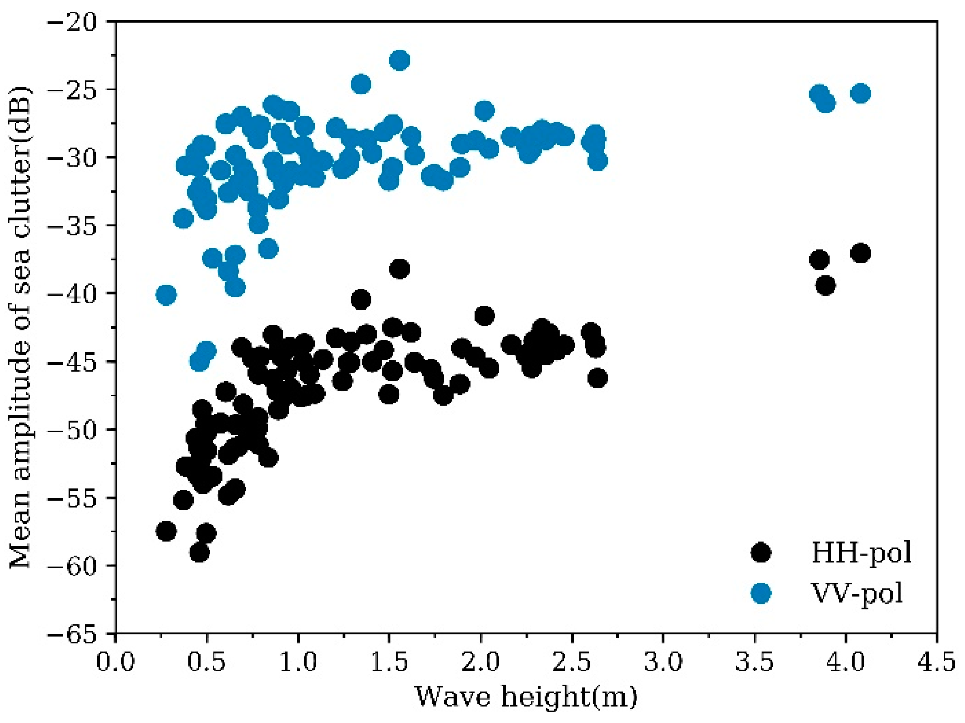
Figure 10 shows the variation in sea clutter amplitude with wave height. It can be seen that the mean amplitude increases with the increase in wave height and gradually reaches the saturation point. This is because the gravity wave generated in this paper is directly related to the wave height. With the increase in wave height, the wave fluctuation will reach saturation. However, with the increase in wind speed, the sea state rapidly increases, and the physical phenomena, such as wave curling, breaking and foam covering, will have a huge impact on the sea clutter, which requires further establishment of the foam scattering mechanism.

Figure 10.
The mean value of different polarized sea clutter amplitudes in the X-band of the Yellow Sea varies with wave height.
In order to further verify the rationality of the mean value of the simulated sea clutter amplitude in this paper, Figure 11 shows the comparison between the calculation results of the mean amplitude value and the actual sea surface measurement results. The measurement data come from the test results of the U.S. Naval Research Laboratory four-band radar in Bermuda, the North Atlantic and the Caribbean, where the X-band frequency is 9.81 GHz [29]. As shown in Figure 11, the comparison results between the simulated data and the X-band radar measured data are in good agreement, and the HH polarization simulation data are smaller than the radar-measured data, due to three reasons: (1) the difference in the marine environment in different sea areas at different times; (2) the multiple scattering mechanism of the small grazing angle is not considered; (3) there may be errors in the experimental data.
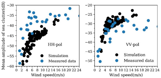
Figure 11.
Comparison of X-band-simulated data and radar-measured data in the Yellow Sea.
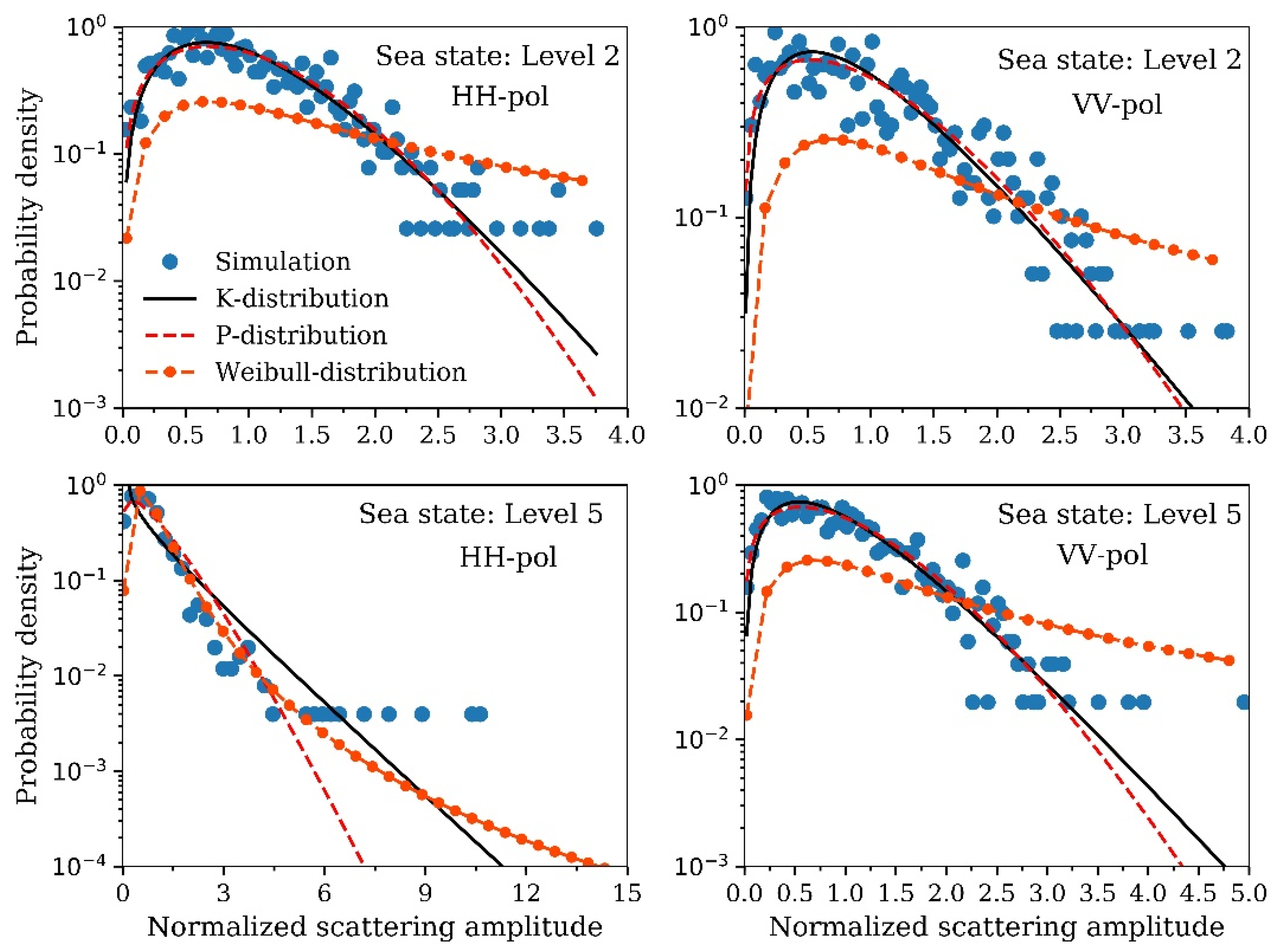
Figure 12 shows the estimated K distribution [30], Pareto distribution [31] and Weibull distribution [32] of the simulated data under different sea conditions and polarizations in the X-band. The normalized scattering coefficient amplitude is obtained by dividing by the data mean, and the number of samples in the amplitude mean data is 1024. It can be seen that both the K distribution and the P distribution can well estimate the distribution of the simulation data. The tailing phenomenon of sea clutter data is more serious under high-frequency and high-sea conditions, especially the HH polarization.

Figure 12.
Probability distribution of mean value of sea clutter amplitude in X-band with different polarization.
4.2. Doppler Spectrum Calculation
Based on the time series of the sea surface scattering field based on the real marine environmental elements, the Doppler spectrum characteristics can be obtained as [32]:
where, refers to the number of sampling samples in the sea surface time series and is the interval time of the time series; is the time-evolving scattering field from the dynamic sea surface.
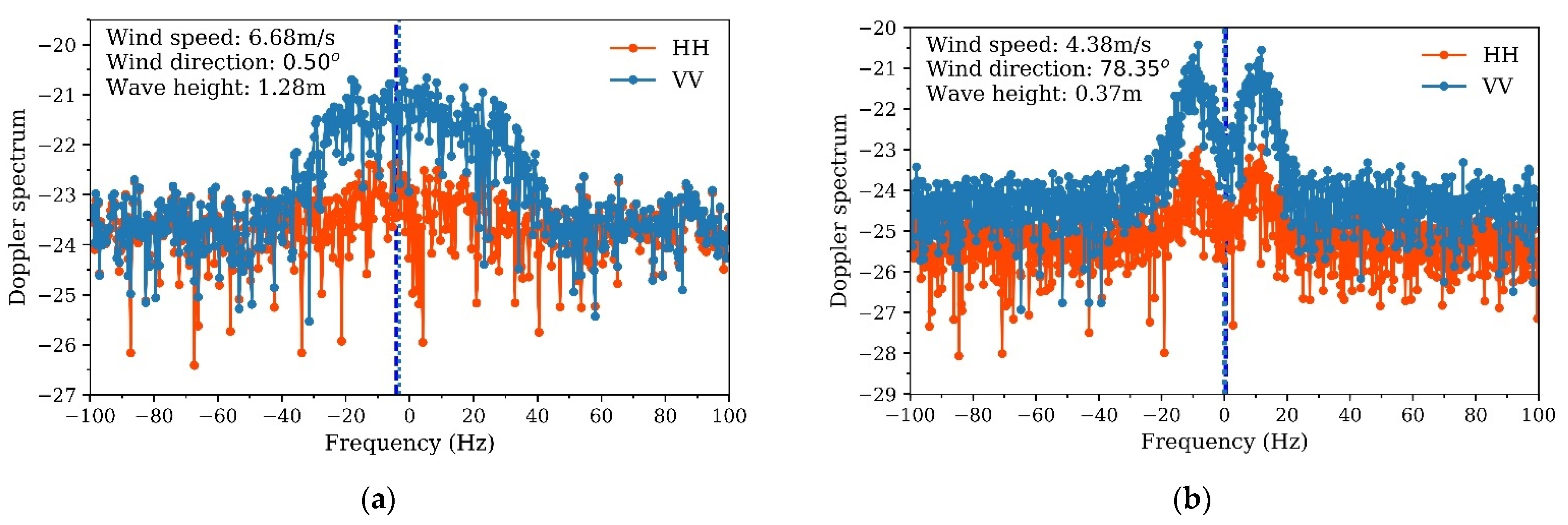
In order to study the influence of wind direction on Doppler spectral characteristics, two special wind direction examples were selected from marine environmental elements. The wind direction angles in Figure 13 correspond to 0.5 degrees and 78.35 degrees, respectively. The radar line-of-sight azimuth is 0 degrees by default. The angle for the calculation example is close to the downwind (0 degree) and the crosswind (90 degree), the value of the marine environment elements is also given in Figure 13 and the grazing angle is 10 degrees. Figure 13 illustrates the Doppler shift and Doppler energy distribution from the negative frequency domain to the positive frequency domain as the wind direction changes from downwind to upwind. In the same sea state, when the incident angle is small, EM scattering from the sea surface is dominated by a quasi-specular scattering mechanism caused by large-scale gravity waves. As the incident angle increases, the Bragg scattering mechanism corresponding to small-scale ripples plays a leading role and the number of facets with contribution to the sea clutter is significantly decreased, which leads to a gradual concentration of Doppler spectrum (dotted line in Figure 13) around the Bragg frequencies (dashed line in Figure 13). Near the crosswind direction, the Doppler frequency is near zero frequency, and two spectral peaks of the Doppler spectrum will be distributed in the positive frequency domain and the negative frequency domain. These distinctive features are consistent with the results in [9].

Figure 13.
Characteristics of Doppler spectrum distribution under different wind directions in X-band. (a) Wind direction: 0.5; (b) Wind direction: 78.35.
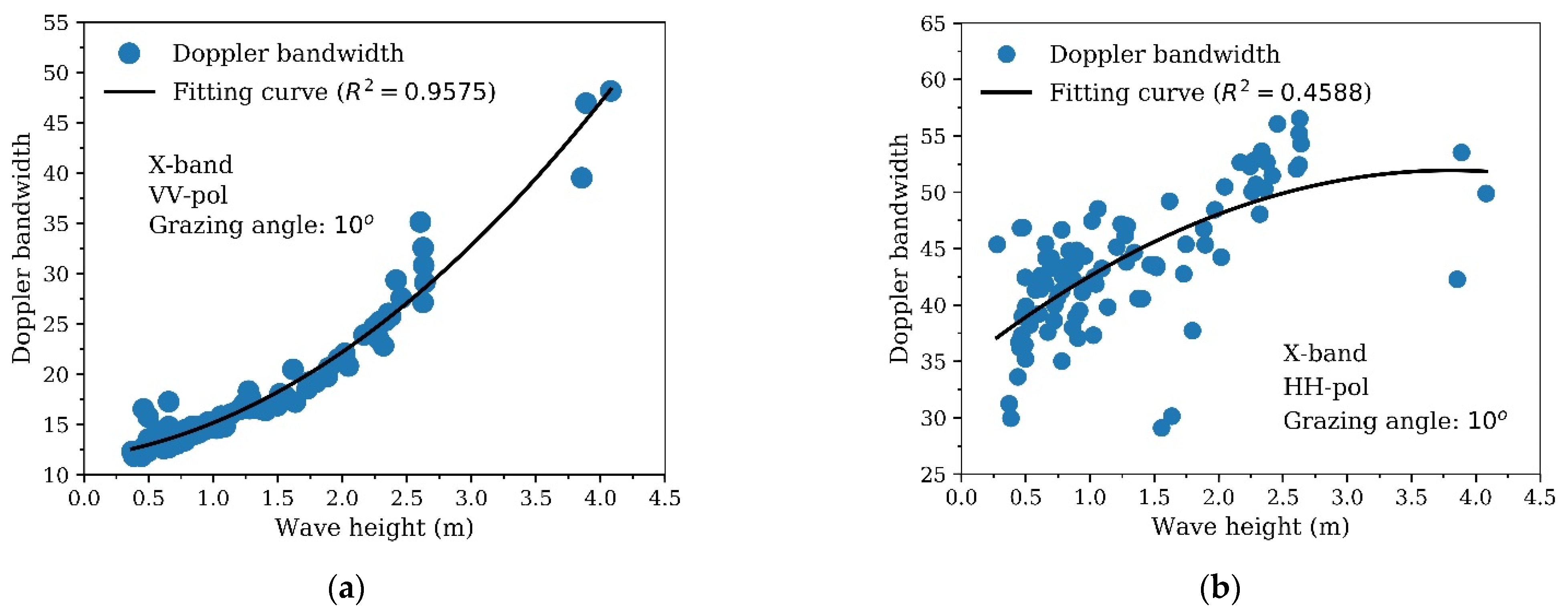
To further illustrate the relationship between sea clutter Doppler characteristics and ocean parameters, Figure 14 shows the variation in Doppler broadening with wave height for different polarizations. In order to quantitatively analyze this relationship, this paper introduces a polynomial to fit the data, and calculates the coefficient of determination of the fitting curve. The closer the coefficient of determination is to 1, the more obvious the positive correlation between the data. As shown in Figure 14, the correlation between spectrum bandwidth and wave height is significantly higher than that with wind speed, and the coefficient of determination of the fitting curve between VV Doppler bandwidth and wave height even reaches 0.9575. For the same set of data, the reason for this result is that the time series sea surface in this paper is established according to the wave height and wave period of the real ocean environment, and the Doppler bandwidth reflects the motion law of the sea surface, so the correlation with the sea surface state will be higher. In addition, the high correlation between Doppler spectrum bandwidth and wave height under VV polarization also brings convenience for wave height inversion based on simulation data results.

Figure 14.
Characteristics of different polarization Doppler spectra in X-band at different wave heights in the Yellow Sea. (a) VV polarization; (b) HH polarization.
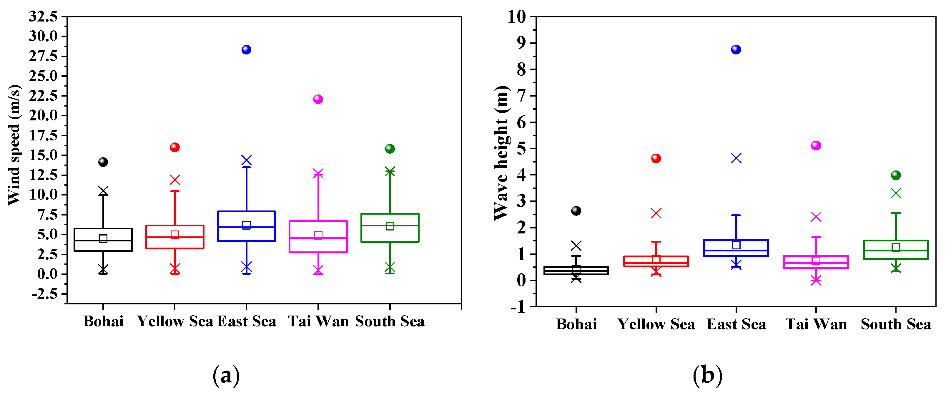
Figure 15 shows the horizontal comparison of the distribution characteristics of wind speed and wave height in different sea areas in summer 2015–2017. As shown in Figure 15, the complex and changeable marine environment in different sea areas will lead to significant differences in sea clutter.
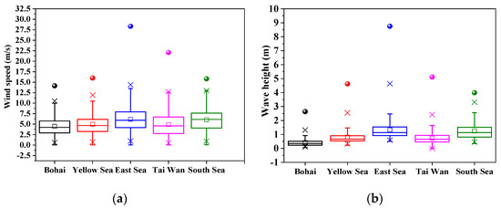
Figure 15.
Box chart statistics of wind speed and wave height in different sea areas in summer 2015–2017. (a) Wind speed; (b) wave height.
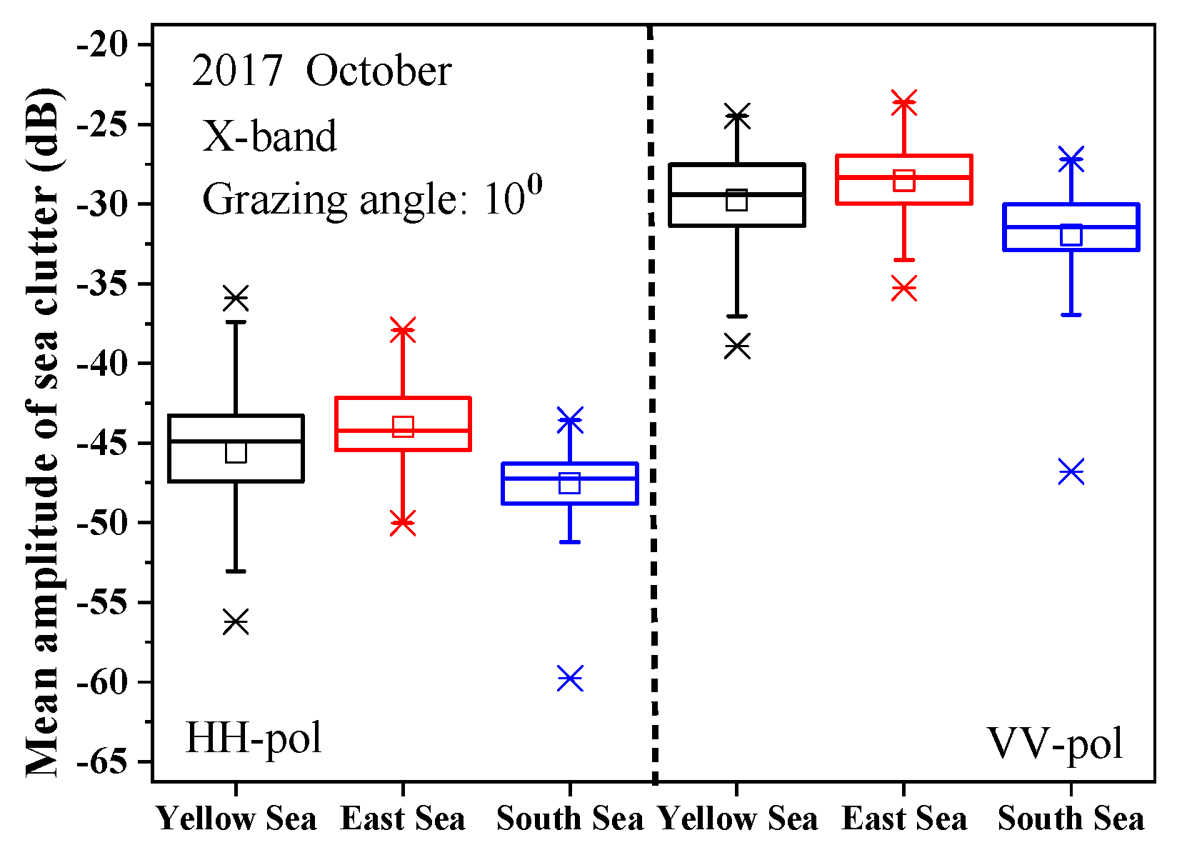
Figure 16 shows the statistical distribution of mean amplitude characteristics under different polarizations in different sea areas. It can be seen from the figure that the statistical characteristics of HH polarization and VV polarization are consistent. However, the mean amplitude of the South China Sea is less than that of the Yellow Sea and the East China Sea, which is due to the low marine environmental factors in the South China Sea. Therefore, the characteristics of sea clutter in different sea areas must be analyzed and studied in combination with specific marine environmental factors.

Figure 16.
Statistics of mean amplitude characteristics under different polarizations in different sea areas.
5. Conclusions
In this paper, a time-varying multi-scale sea surface EM backscattering algorithm and CUDA high-performance parallel computing technology are proposed to establish the sea clutter time series of the sea surface based on real marine environmental elements. Combined with the marine environmental elements of the Yellow Sea in January 2017, the time series of sea clutter under different frequency bands, different polarizations, different sea conditions and different sea areas were calculated. Theoretical analysis shows that the changes in different parameters have a greater impact on the HH-polarized scattering field, especially in the case of high frequency, high sea states and small grazing angles, making the HH polarization more prone to sea peaks in a high-sea state.
A data set of sea clutter characteristics under real marine environmental elements is established. The results not only conform to the laws of the actual sea surface measurement results, especially the phenomenon that the VV polarization scattering coefficient is gradually saturated with the change in wind speed, but also are consistent with the X-band radar measurement results of the US Naval Research Laboratory. The probability distribution of the simulated sea clutter scattering coefficient amplitudes conforms to the K distribution and the Pareto distribution, and with the increase in wind speed, the K distribution obtained from HH polarization scattering amplitude has an obvious downward trend, while the VV polarization scattering has no apparent correlation. There is a relatively obvious correlation between different polarization Doppler bandwidth and wind speed and wave height, especially VV polarization. The determination coefficient of the fitting curve between the VV polarization Doppler bandwidth and wave height obtained by simulation even reaches 0.9575, which has clear guiding significance for the inversion of sea wave information based on sea clutter characteristics.
Author Contributions
Conceptualization, Z.W., J.W. and G.J.; methodology, L.L.; software, L.L. and T.W.; validation, J.W. and Z.W.; formal analysis, L.L.; investigation, J.W.; resources, T.W.; data curation, L.L.; writing—original draft preparation, L.L.; writing—review and editing, J.W.; visualization, L.L.; supervision, Z.W.; project administration, J.W.; funding acquisition, L.L. and J.W. All authors have read and agreed to the published version of the manuscript.
Funding
This research was funded by the National Natural Science Foundation of China, numbers 61901335, Natural Science Basic Research Program of Shannxi, numbers 2020JQ-329.
Data Availability Statement
The data utilized in the analysis were kindly provided by the European Center for Medium-Range Weather Forecasts (ECMWF), (https://www.ecmwf.int, accessed on 20 December 2021).
Acknowledgments
We thank all the editors and reviewers for their valuable comments that greatly improved the presentation of this paper.
Conflicts of Interest
The authors declare no conflict of interest.
References
- Christophe, B. Propagation and Scattering in Ducting Maritime Environments from an Accelerated Boundary Integral Equation. IEEE Trans. Antennas Propagat. 2016, 13, 11–23. [Google Scholar]
- Ma, L.; Wu, J.; Zhang, J. Research on Sea Clutter Reflectivity Using Deep Learning Model in Industry 4.0. IEEE Trans. Ind. Inform. 2020, 16, 5929–5937. [Google Scholar] [CrossRef]
- Voronovich, A.G.; Zavorotny, V.U. Theoretical model for scattering of radar signals in Ku- and C-bands from a rough surface with breaking waves. Waves Random Media 2001, 11, 247–269. [Google Scholar] [CrossRef]
- Fuchs, J.; Regas, D.; Waseda, T.; Welch, S.; Tulin, M.P. Correlation of hydrodynamic features with LGA radar backscatter from breaking waves. IEEE Trans. Geosci. Remote Sens. 1999, 37, 2442–2460. [Google Scholar] [CrossRef]
- Linghu, L.; Wu, J.; Huang, B. GPU-accelerated massively parallel computation of electromagnetic scattering of a time-evolving oceanic surface model I: Time-evolving surface generation. IEEE J. Sel. Top. Appl. Earth Observ. Remote Sens. 2014, 7, 1372–1382. [Google Scholar] [CrossRef]
- Wu, Z.S.; Zhang, J.P.; Guo, L.X.; Zhou, P. An improved two-scale mode with volume scattering for the dynamic ocean surface. Prog. Electromagn. Res. 2009, 89, 39–46. [Google Scholar] [CrossRef] [Green Version]
- Toporkov, J.V.; Brown, G.S. Numerical study of the extended Kirchhoff approach and the lowest order small slope approximation for scattering from ocean-like surface: Doppler analysis. IEEE Trans. Antennas Propag. 2002, 50, 417–425. [Google Scholar] [CrossRef]
- Elfouhaily, T.; Joelson, M.; Guignard, S.; Thompson, D.R. Analytical comparison between the surface current integral equation and the second-order small-slope approximation. Waves Random Media 2003, 13, L711. [Google Scholar] [CrossRef]
- Li, X.; Xu, X. Scattering and Doppler spectral analysis for two-dimensional linear and nonlinear sea surface. IEEE Trans. Geosci. Remote Sen. 2011, 49, 603–611. [Google Scholar] [CrossRef]
- Drennan, W.M.; Graber, H.C.; Hauser, D. On the wave age dependence of wind stress over pure wind seas. J. Geophys. Res. Atmos. 2003, 108, 1–13. [Google Scholar] [CrossRef]
- Edson, J.B.; Crawford, T.; Crescenti, J. The coupled boundary layers and air sea transfer experiment in low winds. Bull. Am. Meteorol. Soc. 2007, 88, 341. [Google Scholar] [CrossRef]
- Li, J.; Zhang, M.; Fan, W.; Nie, D. Facet-based investigation on microwave backscattering from sea surface with breaking waves: Sea spikes and SAR imaging. IEEE Trans. Geosci. Remote Sens. 2017, 55, 2313–2325. [Google Scholar] [CrossRef]
- Chen, H.; Zhang, M.; Zhao, Y.; Luo, W. An efficient slope-deterministic facet model for SAR imagery simulation of marine scent. IEEE Trans. Antennas Propag. 2010, 58, 3751–3756. [Google Scholar] [CrossRef]
- Zhang, M.; Chen, H.; Yin, H.-C. Facet-based investigation on EM scattering from electrically large sea surface with two-scale profile: Theorical model. IEEE Trans. Geosci. Remote Sens. 2011, 49, 1967–1975. [Google Scholar] [CrossRef]
- Linghu, L.; Wu, J.; Wu, Z. GPU-accelerate computation of tiem-evolving electromagnetic backscattering field from large dynamic sea surface. IEEE Trans. Ind. Inform. 2020, 16, 3187–3197. [Google Scholar] [CrossRef]
- Wang, T.; Tong, C. An improved facet-based TSM for Electromagnetic scattering from ocean surface. IEEE Trans. Geosci. Remote Sens. 2018, 15, 644–648. [Google Scholar] [CrossRef]
- Clarizia, M.P.; Gommenginger, C.; Bisceglie, M.D. Simulation of L-band bistatic returns from the ocean surface: A facet approach with application to ocean GNSS reflectometry. IEEE Trans. Geosic. Remote Sens. 2012, 50, 960–971. [Google Scholar] [CrossRef]
- Su, X.; Wu, J.; Huang, B.; Wu, Z. GPU-accelerated computation for electromagnetic scattering of a double-layer vegetation model. IEEE J. Sel. Top. Appl. Earth Observ. Remote Sens. 2013, 6, 1799–1860. [Google Scholar] [CrossRef]
- Wu, J.; Deng, L.; Jeon, G. Image autoregressive interpolation model using GPU-parallel optimization. IEEE Trans. Ind. Inform. 2017, 14, 426–436. [Google Scholar] [CrossRef]
- Stopa, J.E.; Cheung, K.F. Intercomparison of wind and wave data from the ECMWF Reanalysis Interim and the NCEP Climate Forecast System Reanalysis. Ocean. Model. 2014, 75, 65–83. [Google Scholar] [CrossRef]
- Kerr, Y.H.; Waldteufel, P.; Wigneron, J.P. Soil moisture retrieval from space: The Soil Moisture and Ocean Salinity (SMOS) mission. IEEE Trans. Geosci. Remote Sens. 2002, 39, 1729–1735. [Google Scholar] [CrossRef]
- Torsethaugen, K.; Haver, S. Simplified double peak spectral model for ocean waves. In Proceedings of the The Fourteenth International Offshore and Polar Engineering Conference, Toulon, France, 23–28 May 2004; pp. 1–9. [Google Scholar]
- Panahi, R.; Ghasemi, A.K.; Shafieefar, M. Development of a bi-modal directional wave spectrum. Ocean. Eng. 2015, 105, 104–111. [Google Scholar] [CrossRef]
- Joung, S.J.; Shelton, J. 3 Dimensional ocean wave model using directional wave spectra for limited capacity computers. In Proceedings of the IEEE OCEANS 91 Ocean Technologies and Opportunities in the Pacific for the 90s, Honololu, HI, USA, 1–3 October 1991; p. 1. [Google Scholar]
- Chen, K.S.; Fung, A.K.; Weissman, D.E. A backscattering model for ocean surface. IEEE Trans. Geosci. Remote Sens. 1991, 30, 811–817. [Google Scholar] [CrossRef]
- Hsu, W.; Barakat, R. Stratton-Chu vectorial diffraction of electromagnetic fields by apertures with application to small-Fresnel-number system. J. Opt. Soc. Am. A 1994, 11, 623–629. [Google Scholar] [CrossRef]
- Fuks, I.M. Wave diffraction by a rough boundary of an arbitrary plane-layered medium. IEEE Trans. Antennas Propagat. 2001, 49, 630–639. [Google Scholar] [CrossRef]
- Keller, W.C.; Plant, W.J.; Petitt, R.A. Microwave backscatter from the sea: Modulation of received power and Doppler bandwidth by long waves. J. Geophys. Res. 1994, 99, 9751–9766. [Google Scholar] [CrossRef]
- Daley, J.C. Radar Sea Return-JOSS I; Naval Research Lab: Washington DC, USA, 1971. [Google Scholar]
- Watts, S.; Ward, K.; Tough, R. Modelling the shape parameter of sea clutter. In International Radar Conference-Surveillance for a Safer World; RADAR: Red Hook, NY, USA, 2009; pp. 1–6. [Google Scholar]
- Farshchian, M.; Posner, F.L. The Pareto distribution as a model for high grazing angle clutter. In Proceedings of the IEEE Radar Conference, Arlington, VA, USA, 10–14 May 2010; pp. 789–793. [Google Scholar]
- Toporkov, J.V.; Brown, G.S. Numerical simulation of scattering from time-varying, randomly rough surface. IEEE Trans. Geosci. Remote Sens. 2000, 38, 1616–1625. [Google Scholar] [CrossRef]


Publisher’s Note: MDPI stays neutral with regard to jurisdictional claims in published maps and institutional affiliations. |
© 2022 by the authors. Licensee MDPI, Basel, Switzerland. This article is an open access article distributed under the terms and conditions of the Creative Commons Attribution (CC BY) license (https://creativecommons.org/licenses/by/4.0/).