Inversion of Coniferous Forest Stock Volume Based on Backscatter and InSAR Coherence Factors of Sentinel-1 Hyper-Temporal Images and Spectral Variables of Landsat 8 OLI

Abstract

Forest stock volume (FSV) is a basic data source for estimating forest carbon sink. It is also a crucial parameter that reflects the quality of forest resources and forest management level. The use of remote sensing data combined with a support vector regression (SVR) algorithm has been widely used in FSV estimation. However, due to the complexity and spatial heterogeneity of the forest biological community, in the FSV high-value area with dense vegetation, the optical re-mote sensing variables tend to be saturated, and the sensitivity of synthetic aperture radar (SAR) backscattering features to the FSV is significantly reduced. These factors seriously affect the ac-curacy of the FSV estimation. In this study, Landsat 8 (L8) Operational Land Imager multispectral images and C-band Sentinel-1 (S1) hyper-temporal SAR images were used to extract three re-mote sensing feature datasets: spectral variables (L8), backscattering coefficients (S1), and inter-ferometric SAR factors (S1-InSAR). We proposed a feature selection method based on SVR (FS-SVR) and compared the FSV estimation performance of FS-SVR and stepwise regression analysis (SRA) on the aforementioned three remote sensing feature datasets. Finally, an estima-tion model of coniferous FSV was constructed using the SVR algorithm in Wangyedian Forest Farm, Inner Mongolia, China, and the spatial distribution map of coniferous FSV was predicted. The experimental results show the following: (1) The coherence amplitude and DSM data ob-tained based on S1 images contain information relat-ed to forest canopy height, and the hy-per-temporal S1 image data significantly enrich the diversity of S1-InSAR feature factors. There-fore, the S1-InSAR dataset has a better FSV response than remote sensing factors such as the S1 backscattering coefficient and L8 vegetation index, and the corresponding root mean square er-ror (RMSE) and relative RMSE (rRMSE) values reached 47.6 m³/ha and 20.9%, respectively. (2) The integrated dataset can provide full play to the synergy of the L8, S1, and S1-InSAR remote sensing data. Its RMSE and rRMSE values are 44.3 m³/ha and 19.4% respectively. (3) The proposed FS-SVR method can better select remote sensing variables suitable for FSV estimation than SRA. The average value of the rRMSE (23.17%) based on the three datasets was 13.8% lower than that of the SRA method (26.87%). This study provides new insights into forest FSV retrieval based on active and passive multisource remote sensing joint data.

1. Introduction

The carbon stored through forest ecosystems accounts for about 2/3 of the total carbon pool of the whole terrestrial ecosystems [1,2]. Forest stock volume (FSV) is a basic data source for estimating forest biomass and the carbon sink. It is also a crucial parameter that reflects the quality of forest resources and forest management level [3,4,5]. The dynamic estimation of the spatial distribution of FSV is not only the basis of scientific and accurate forest management, but also the prerequisite for maximizing the function and carbon se-questration potential of forest ecosystems [6,7,8].

Although many large-scale global products can easily obtain FSV information, the use of specific areas is easily limited by time-frequency, spatial resolution, or other un-known local errors [9,10,11,12,13,14,15]. Due to the strong spatial heterogeneity of forest ecosystems, the response relationship between remote sensing factors and FSV is usually complex [16,17]. Many problems remain in the research and application of FSV estimation based on remote sensing technology. Optical remote sensing is a passive remote sensing technology. In the densely vegetated high-value area of the FSV, optical remote sensing technology cannot obtain the spectral signal of the inner section of the forest and the vertical direction of the canopy; therefore, problems such as poor spectral sensitivity and low light saturation point are observed [18,19,20,21,22,23]. LiDAR is an emerging active remote sensing technology [24,25,26,27,28,29,30]. However, few spaceborne data are available, the cost of airborne data acquisition is high, which limits its widespread application in the field of FSV remote sensing estimation [20]. Microwave radar is an advanced active remote sensing technology not easily affected by climatic factors, such as clouds, fog, and solar radiation, and can realize all-weather earth observations [31,32,33]. Depending on the wavelength and frequency, microwave radar signals can penetrate the forest canopy to different degrees and obtain comprehensive in-formation on the forest structure at different levels and orientations [34,35,36,37,38,39]. The micro-wave radar remote sensing technologies commonly used in FSV estimation include syn-thetic aperture radar (SAR), interferometric radar (InSAR), and polarization interferomet-ric radar (PolInSAR) [40,41].

The microwave radar backscattering coefficient and its textural features have been widely used in research on FSV and forest aboveground biomass (AGB) [39,42]. Erkki et al. [43] used Sentinel-1 C-band SAR to conduct a forest snow damage mapping study in northern and southern Finland, with an overall accuracy of 90%. They also estimated the FSV in damaged forest areas, and the results suggested that multitemporal Sentinel-1 data have good potential for estimating the overall FSV. In research on FSV estimation based on C-band-and L-band SAR images, the findings of Tanase et al. [44] demonstrated that the FSV estimation performance of C-band and L-band SAR data is almost the same, and the synergy between the two data is limited. Purohit et al. [40] used Landsat 8 OLI and Senti-nel-1A images to accurately predict the spatial distribution of AGB of different forest types in the foothills of the Indian Himalayas, indicating that the coordination of optical remote sensing variables and radar backscatter data can effectively improve the accuracy of forest AGB estimation. Using InSAR technology to perform radar signal interferometric processing on two SAR complex images can generate an interferometric phase, interferometric coherence coefficient, digital surface model (DSM), and other feature factors that contain information on the horizontal and vertical structures of the forest, which are usually very beneficial for FSV estimation [42]. Borlafmena et al. [45] assessed the utility of Sentinel-1 coherence time series for temperate and tropical forest mapping. They found that for forest classification on rough terrain, the Sentinel-1 coherence amplitude can significantly reduce the error of forest missions. In addition, Sentinel-1 time series data based on InSAR technology have shown excellent performance in the research of land subsidence, surface deformation monitoring, and post-disaster assessment [41,46,47,48,49]. Sentinel-1 imagery has the advantages of global coverage, free access, and high spatial and temporal resolution [42,45]; however, the full potential of Sentinel-1 C-band interferometry SAR (S1-InSAR) coherent data for estimating boreal FSV has rarely been studied. In addition, the Sentinel-1 backscattering coefficient, InSAR coherence coefficient, and Landsat 8 OLI spectral feature variables were not used together to predict FSV.

The selection of remote sensing feature variables is a key factor in determining the accuracy of the FSV estimation model [20,50,51,52,53]. The random forest (RF) method can evaluate and rank the importance of remote sensing features by using the out-of-bag esti-mation error before and after adding noise to the feature variables; however, it does not consider the combination effect relationship between the feature variables [10,12,50]. Stepwise regression analysis (SRA) can dynamically eliminate redundant features through a variance homogeneity test; however, it can only select variables based on the linear relationship between remote sensing variables and FSV [10]. The support vector regression (SVR) algorithm is a classical small-sample learning method with a profound theoretical foundation. It has a satisfactory generalization performance, is resilient to overfit, and can achieve good estimation performance in the case of very few sample data. Therefore, this method has been widely used for remote sensing monitoring and modeling of forest resources [20,52,54]. However, few studies have used the SVR algorithm combined with the combination effect of remote sensing feature variables to select remote sensing variables.

Therefore, this study will build a coniferous plantation FSV remote sensing inversion experimental area in northern China. Based on sentinel-1 SAR backscattering coefficient, hyper temporal InSAR coherence factors and Landsat 8 spectral variables, SVR algorithm combined with the combination effect of remote sensing characteristic variables will be used to select remote sensing variables and build FSV estimation model, so as to effective-ly improve the estimation accuracy of coniferous forest volume through the combination of active and passive remote sensing data.

2. Study Area and Data

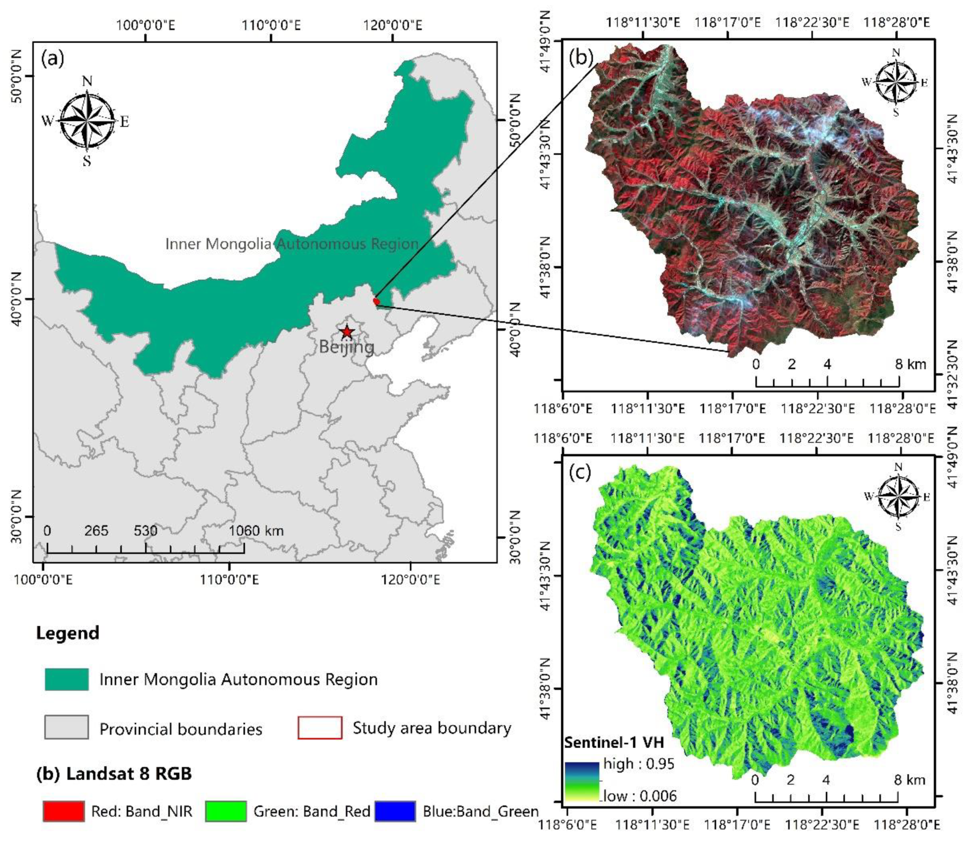
2.1. Study Area

The study area, the Wangyedian Forest Farm, with a forest area of 23,118 ha, is located in Harqin, Inner Mongolia Autonomous Region, Northeast China (118°09′ to 118°30′E, 41°21′ to 41°39′N) (Figure 1). This choice was influenced by the temperate monsoon climate as well as the annual precipitation, temperature, and the frost-free period of the study area, which are, approximately, 400 mm, 4.2 °C, and 117 d, respectively. There are many rolling mountains, with an altitude distribution of 800–1890 m, on the forest farm. The forest farm is rich in forest resources and beautiful scenery, with a total FSV of 1.5 million m³, of which the FSV of the plantation is approximately 0.8 million m³. It has a forest area of 350,000 mu, including 176,000 mu of planted forest, and the main tree species are larch (Larix gmelinii Kuzen.) and Chinese pine (Pinus tabuliformis Carrière). The natural forest area is 174,000 mu, and the main tree species are white birch (Betula platyphylla Suk.), aspen (Populus davidiana Dode) and oak (Xylosma racemosum Miq.) [12].

2.2. Sample Plot Design and FSV Data Collection

The setting of the FSV sample plot was selected according to many factors, including altitude, slope direction, slope, and stand age structure. Each sample plot had a size of 25 × 25 m, was required to contain only one main forest type, and was far from the stand boundary. For fulfilling the needs of high-precision positioning and measurement, the investigators used the RTK to collect the coordinate position and terrain information in the sample plot and measured the height of trees in the sample plot with a laser altimeter; the DBH of all living trees with a DBH greater than or equal to 5 cm in the sample plot was measured with a special DBH ruler (1.3 m from the ground). The collected data included information on tree species, DBH, tree height, crown width, and the height of trees under branches, as well as the geographical environment data of the sample plot, such as the coordinates of the central point of the sample plot, altitude, slope, and slope direction.

The fieldwork inventory was conducted in the autumn of 2017 and 2019, and there were 54 larch and 76 Chinese pine sample plots (Figure 2). Using the FSV calculation formula for larches and Chinese pines provided by the forest farm (

Table 1. Coniferous forest stock volume calculation formulas in the study area.

Tree Species	FSV Calculation Formula	Remarks
Larch	FSV= −0.001498 + 0.00007 × D2 + 0.000901 × H + 0.000032 × H × D2	D: DBH H: Tree height
Chinese pine	FSV= 0.013464 − 0.001967 × D + 0.000089 × D2 + 0.000628 × D × H + 0.000032 × H × D2 − 0.003173 × H

), the stock volume of each tree in the sample plot was calculated. According to the growth curves of tree height and the DBH of larches and Chinese pines at different age levels, the corresponding annual relative growth was calculated to convert the FSV in 2017 into the FSV in 2019. The final FSV data from the 130 sample plots were summarized and converted into hectares (m³/ha) (

Table 2. Statistical summary of forest stock volume (m³/ha) at field plots.

Tree Species	Numbers of Plots	Minimum	Maximum	Mean	Standard Deviation	Coefficient of Variation (%)
Chinese pine	76	105	519	230.8	83.2	36.1
Larch	54	76	360	223.4	63.5	28.4
All	130	76	519	227.7	75.5	33.2

).

2.3. Optical and SAR Remote Sensing Data Preprocessing

One Landsat 8 (L8) and thirty-nine Sentinel-1 (S1) hyper-temporal images (

Table A1. Landsat 8 and Sentinel-1 image information covering the Wangyedian research area used in this study.

Image Category	Image Identification	Acquisition Date
Landsat 8	LC08_L1TP_122031_20190927_20191017_01_T1	20190927
Sentinel-1B	S1B_IW_SLC__1SDV_20191230T221132_20191230T221159_019600_0250B0_2899	20191230
	S1B_IW_SLC__1SDV_20191218T221133_20191218T221200_019425_024B1B_4D83	20191218
	S1B_IW_SLC__1SDV_20191206T221133_20191206T221200_019250_024587_75B0	20191206
	S1B_IW_SLC__1SDV_20191124T221134_20191124T221201_019075_023FFC_F9D2	20191124
	S1B_IW_SLC__1SDV_20191112T221134_20191112T221201_018900_023A5C_5D48	20191112
	S1B_IW_SLC__1SDV_20191019T221134_20191019T221201_018550_022F3E_5B86	20191019
	S1B_IW_SLC__1SDV_20191007T221134_20191007T221201_018375_0229DE_E289	20191007
	S1B_IW_SLC__1SDV_20190925T221134_20190925T221201_018200_022459_AE9B	20190925
	S1B_IW_SLC__1SDV_20190901T221133_20190901T221200_017850_02197D_522E	20190901
	S1B_IW_SLC__1SDV_20190820T221132_20190820T221159_017675_02140F_526D	20190820
	S1B_IW_SLC__1SDV_20190810T095659_20190810T095725_017522_020F3E_BC60	20190810
	S1B_IW_SLC__1SDV_20190808T221132_20190808T221159_017500_020E97_6E25	20190808
	S1B_IW_SLC__1SDV_20190727T221131_20190727T221158_017325_02094E_08A7	20190727
	S1B_IW_SLC__1SDV_20190715T221130_20190715T221157_017150_020438_6966	20190715
	S1B_IW_SLC__1SDV_20190703T221129_20190703T221156_016975_01FF10_9955	20190703
	S1B_IW_SLC__1SDV_20190621T221129_20190621T221156_016800_01F9E2_C83C	20190621
	S1B_IW_SLC__1SDV_20190609T221128_20190609T221155_016625_01F4AC_6072	20190609
	S1B_IW_SLC__1SDV_20190528T221127_20190528T221154_016450_01EF78_A431	20190528
	S1B_IW_SLC__1SDV_20190516T221127_20190516T221154_016275_01EA17_1542	20190516
	S1B_IW_SLC__1SDV_20190504T221126_20190504T221153_016100_01E499_637A	20190504
	S1B_IW_SLC__1SDV_20190422T221126_20190422T221153_015925_01DEBD_37CA	20190422
	S1B_IW_SLC__1SDV_20190329T221125_20190329T221152_015575_01D321_91C4	20190329
	S1B_IW_SLC__1SDV_20190317T221124_20190317T221151_015400_01CD68_5402	20190317
Sentinel-1A	S1A_IW_SLC__1SDV_20191226T095744_20191226T095812_030518_037E99_1211	20191226
	S1A_IW_SLC__1SDV_20191214T095744_20191214T095812_030343_037891_1BF4	20191214
	S1A_IW_SLC__1SDV_20191202T095745_20191202T095813_030168_037286_5B2A	20191202
	S1A_IW_SLC__1SDV_20191120T095745_20191120T095813_029993_036C78_D64C	20191120
	S1A_IW_SLC__1SDV_20191108T095745_20191108T095813_029818_036669_AAD4	20191108
	S1A_IW_SLC__1SDV_20191015T095745_20191015T095813_029468_035A34_B673	20191015
	S1A_IW_SLC__1SDV_20190921T095745_20190921T095813_029118_034E23_9420	20190921
	S1A_IW_SLC__1SDV_20190909T095745_20190909T095812_028943_034826_7BA8	20190909
	S1A_IW_SLC__1SDV_20190828T095744_20190828T095812_028768_034210_B0B1	20190828
	S1A_IW_SLC__1SDV_20190816T095743_20190816T095811_028593_033BF0_21BC	20190816
	S1A_IW_SLC__1SDV_20190804T095743_20190804T095811_028418_033619_59BC	20190804
	S1A_IW_SLC__1SDV_20190723T095742_20190723T095810_028243_0330C2_ECFE	20190723
	S1A_IW_SLC__1SDV_20190711T095741_20190711T095809_028068_032B79_A792	20190711
	S1A_IW_SLC__1SDV_20190629T095740_20190629T095808_027893_03262C_B424	20190629
	S1A_IW_SLC__1SDV_20190617T095739_20190617T095807_027718_0320F1_5DB1	20190617
	S1A_IW_SLC__1SDV_20190605T095739_20190605T095807_027543_031BAA_448C	20190605

) were obtained from the United States Geological Survey (https://earthexplorer.usgs.gov/) (accessed on 9 May 2021) and the European Space Agency Copernicus data center (https://scihub.copernicus.eu/) (accessed on 11 July 2021), respectively. Digital elevation model (DEM) data covering the study area were downloaded from the geospatial data cloud (http://www.gscloud.cn/) (accessed on 8 May 2019). They were generated using ASTER GDEM data processing, with a spatial resolution of 30 m, a projection type of UTM/WGS84, and a data type of IMG. We also obtained the forest resource distribution map, administrative boundary vector map, and other relevant auxiliary information pro-vided by the forest farm.

The acquired Landsat 8 Operational Land Imager (OLI) images (level-1T) underwent systematic radiometric and geometric corrections. The spectral information of the forest vegetation can be obtained from OLI images. However, to quantitatively retrieve forest FSV data using image spectral variables, Landsat 8 level-1T products usually need preprocessing, such as radiation calibration and atmospheric correction [10]. Sentinel-1 was the first C-band dual-polarization SAR satellite developed by the Copernicus program of the European Space Agency. Sentinel-1 A and Sentinel-1 B were successfully launched in April 2014 and 2016, respectively. Sentinel-1 images have the advantages of ultrahigh radiation resolution (1 dB/3σ), global coverage, free download, and high spatial resolution. Therefore, Sentinel-1 is widely used in all-weather and all-time radar imaging Earth observation missions [42,47]. The flight orbit space of the Sentinel-1 interferometric wide amplitude mode (IW) is a pipe with a radius of approximately 50 m, and it generates three sub-band (IW1, IW2, IW3) data through progressive terrain scanning to ensure that the interferometric image data have good coherence; thus, it can be used to conduct effective radar interferometric analysis [42,55]. This study obtained 39 Sentinel-1 level-1 IW PolSAR images covering the Wangyedian Forest Farm from March to December 2019 (Table A1), which were single-view complex (SLC) products based on the raw data of the radar system after fast-focusing processing. Sentinel-1 SLC images require a series of processes, such as orbit correction, radiometric calibration, multi-looking, polarization filtering, terrain correction, and geocoding, to obtain a SAR backscattering coefficient. In addition, the 39 hyper-temporal SLC images can be used to form multiple image pairs, and canopy elevation data and coherent information can be obtained through InSAR technology.

3. Methods

3.1. Optical Remote Sensing Feature Variable Extraction

In research on forest FSV estimation based on optical images, the usually extracted optical remote sensing factors mainly include spectral band reflectance, a vegetation index, and texture feature factors extracted by image spatial texture analysis [10,21]. The vegetation index can realize the simple and effective measurement of surface vegetation growth trends, health status, and other information [12,20]. Through texture analysis, the periodic changes of the arrangement and combination attributes of texture primitives at the gray level of the image can be reflected macroscopically [56,57,58,59]. A gray level concurrency matrix (GLCM) is a typical statistical method for texture information analysis [52].

In total, 276 optical remote sensing feature variables were extracted from the L8 OLI images for forest FSV estimation (

Table 3. Optical remote sensing feature variables extracted from L8 OLI image.

Variable Type	Variable Name	Variable Description
Band reflectance	Band i, (i = 1, …, 7)	Band 1: Coastal, Band 2: Blue, Band 3: Green, Band 4: Red, Band 5: NIR, Band 6: SWIR 1, Band 7: SWIR 2
Vegetation indices	NDVI	(Nir − Red)/(Nir + Red)
	RVI_ij	Band i/Band j, i ≠ j
	DVI_ij	Band i/Band j, i ≠ j
	EVI	2.5 × (NIR − Red)/(NIR + 6 × Red − 7.5 × Blue + 1)
	SAVI	(Nir − Red)(1 + 0.5)/(Nir + Red + 0.5)
Texture (GLCM)	Mean (M)	${{\displaystyle \sum }}_{i,j=0}^{ n-1}i{P}_{i,j}$
	Variance (Var)	${{\displaystyle \sum }}_{i,j=0}^{ n-1}{P}_{i,j}\left(i,j-{\mu }_{i,j}\right)$
	Contrast (Con)	${{\displaystyle \sum }}_{i,j=0}^{ n-1}{P}_{i,j}{\left(i-j\right)}^2$
	Homogeneity (Hom)	${{\displaystyle \sum }}_{i,j=0}^{ n-1}{P}_{i,j}/\left(1+{\left(i-j\right)}^2\right)$
	Entropy (Ent)	${{\displaystyle \sum }}_{i,j=0}^{ n-1}{P}_{i,j}\left(-\ln P_{i,j}\right)$
	Dissimilarity (Dis)	${{\displaystyle \sum }}_{i,j=0}^{ n-1}{P}_{i,j}\left|i-j\right|$
	Second Moment (SM)	${{\displaystyle \sum }}_{i,j=0}^{ n-1}{\left(P_{i,j}\right)}^2$
	Correlation (Cor)	${{\displaystyle \sum }}_{i,j=0}^{ n-1}{P}_{i,j}\left(\left(i-{\mu }_i\right)\left(j-{\mu }_j\right)/\sqrt{{\sigma }_i^2{\sigma }_j^2}\right)$

Note: $P_{i,j}=V_{i,j}/{{\displaystyle \sum }}_{i,j=0}^{n-1}{V}_{i,j}$, is the normalized value of element $V_{i,j}$ in row i and column j of the GLCM, and N is the number of rows (columns) in the matrix.

); among them, there were 7 multispectral bands, 45 vegetation index feature variables, and 224 texture feature factors. GLCM was used to obtain image texture information, such as the mean, variance, and homogeneity [13]. As shown in Table 3, based on the GLCM method, texture feature data were extracted from seven multispectral bands of the L8 OLI image, with a sliding window of 3 × 3, 5 × 5, 7 × 7, 9 × 9, and step size of [1,1].

3.2. SAR Feature Variable Extraction

In the microwave radar remote sensing system, ground object types usually include discrete targets, distributed targets, and targets that combine discrete and distributed tar-gets, whereas forests usually belong to the third type of targets. For non-discrete targets, such as forests and farmland, the radar image unit pixel usually contains many scatterers; therefore, the radar echo signal is formed by the coherent superposition of all scatterer signals [39]. Such coherently superimposed scattered signals usually indicate the absence of dominant scatterers; therefore, the concept of the backscattering coefficient needs to be introduced to describe them [41]. The backscattering coefficient is the reflectivity of the radar electromagnetic wave signal per unit of the backscattering cross-sectional area. It describes the interaction between the incident radar electromagnetic waves and ground objects by using statistical methods to measure the scattering ability of ground objects [46]. As shown in Equation (1), the backscattering coefficient Sigma⁰ (σ⁰) can be expressed as the average scattering cross-section corresponding to the unit-effective scattering unit area, which is a dimensionless quantity [39,42,44].

$${\sigma }^0=\sigma /Are{a}_{\sigma }$$

(1)

where 〈σ〉 is the average scattering cross-section of the radar, and $Are{a}_{\sigma }$ is the effective scattering area in the ground distance direction. In a specific application, the unit-effective scattering unit area can also be expressed as the effective scattering unit area $Are{a}_{\gamma }$. perpendicular to the incident direction or the effective scattering unit area $Are{a}_{\beta }$ in the oblique distance direction.

$$Are{a}_{\beta }=Resolutio{n}_r\times Resolutio{n}_a=(c\times \tau /2)\times (D/2)$$

(2)

$$Are{a}_{\sigma }=Resolutio{n}_r\times Resolutio{n}_a/\sin \theta =c\times \tau \times D/4\sin {\theta }^{ }$$

(3)

$$Are{a}_{\gamma }=Resolutio{n}_r\times Resolutio{n}_a/\tan \theta =c\times \tau \times D/4\tan {\theta }^{ }$$

(4)

where $Resolutio{n}_r$ and $Resolutio{n}_a$ are the range and azimuth resolutions of the image, respectively, c is the speed of light, τ is the pulse duration of the radar system, D is the radar aperture size, and θ is the ground-incident angle corresponding to the image pixel. Therefore, the backscattering coefficient can be expressed in the form of Gamma⁰ (γ⁰) and Beta⁰ (β⁰). The radar feature variables extracted from Sentinel-1 SAR images in this paper are shown in

Table 4. Radar feature variables extracted from Sentinel-1 SAR image.

Variable Type	Variable Description
Backscattering coefficients	VV(Sigma0), VH(Sigma0), VV(Gamma0), VH(Gamma0), VV(Beta0), VH(Beta0)
Radar indices	(VH − VV)/(VH + VV), VV/VH
Texture features extracted from Backscattering coefficients	Mean (M), Variance (Var), Homogeneity (Hom), Contrast (Con), Dissimilarity (Dis), Entropy (Ent), Second moment (SM), Correlation (Cor)

Note: VV and VH are the backscattering coefficients corresponding to the polarization modes of VV and VH, respectively; the sliding window scale for extracting texture features based on the backscattering coefficients is (3 × 3, 5 × 5, 7 × 7, 9 × 9, 11 × 11, 13 × 13, 15 × 15).

.

$${\gamma }^0=\sigma /Are{a}_{\gamma }$$

(5)

$${\beta }^0=\sigma /Are{a}_{\beta }$$

(6)

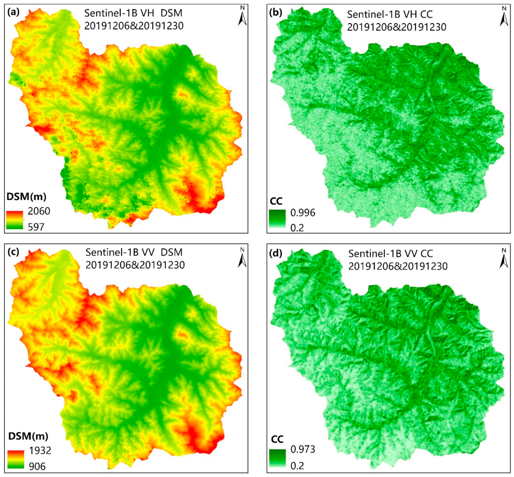
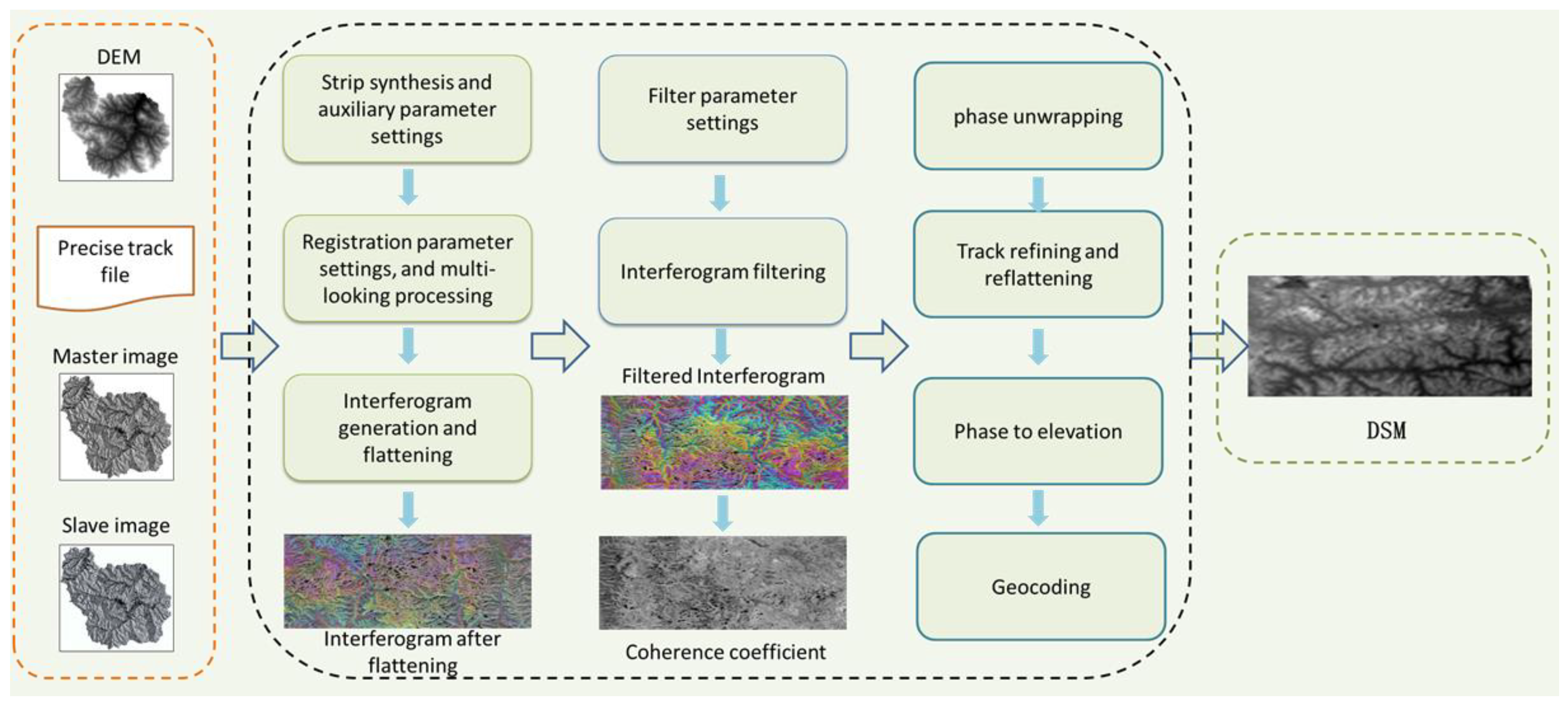
3.3. InSAR Feature Variable Extraction

InSAR is a space–Earth observation technology developed from traditional microwave radar remote sensing technology combined with radio astronomical interferometry [45,46]. Based on the microwave signals transmitted and received by the InSAR system from the target area, SAR complex image pairs containing intensity and the phase information of ground objects in the same area can be generated. If there are coherence conditions between the complex image pairs, an interferogram can be generated using conjugate multiplication. The distance difference between the microwaves can be calculated according to the phase value of the interferogram. The distance information between the ground object target and the sensor can be obtained using parameters such as the flight altitude information of the satellite sensor, the frequency of the microwave radar, and the beam direction; consequently, elevation information corresponding to each pixel target in the SAR image can be measured accurately [48,49].

In this study, the VV and VH polarization data of Sentinel-1 SLC images were used for interference processing. As shown in Figure 3, in the process of interference processing using SNAP software, the downloaded DEM and the boundary shape file of the study area must be used to register and cut the Sentinel-1 image pair. The ratio of the distance view to the azimuth view was set to 5:1, and the mapping resolution was approximately 30 m. The Goldstein algorithm was selected as the filtering method of the interferogram, which not only improved the definition of the interference fringe but also effectively reduced the incoherent noise caused by errors. The phase unwrapping method uses the minimum cost flow method to mask pixels whose coherence is less than the threshold. A polynomial optimization method was used for orbit refining and phase offset correction. Based on the selected control points, re-flattening processing was conducted. Finally, geographic coding was conducted while referring to the DEM image coordinate system to obtain the DSM and the coherence coefficient map.

As shown in

Table A2. Pairing of 39 Sentinel-1 IW SLC images covering Wangyedian study area in 2019.

Number	Paired Image	Satellite and Track	Vertical Baseline Length (m)	Time Baseline Interval (Days)	Interference Processing
1	20190317 and 20190329	S1B-Descending	12.462	12	No
2	20190317 and 20190422	S1B-Descending	46.479	36	Yes
3	20190329 and 20190422	S1B-Descending	58.387	24	Yes
4	20190422 and 20190504	S1B-Descending	81.720	12	Yes
5	20190422 and 20190516	S1B-Descending	35.526	24	Yes
6	20190504 and 20190516	S1B-Descending	48.376	12	Yes
7	20190504 and 20190528	S1B-Descending	74.800	24	Yes
8	20190516 and 20190528	S1B-Descending	26.943	12	Yes
9	20190605 and 20190617	S1A-Ascending	46.979	12	Yes
10	20190609 and 20190621	S1B-Descending	55.835	12	Yes
11	20190617 and 20190629	S1A-Ascending	74.956	12	Yes
12	20190621 and 20190703	S1B-Descending	91.912	12	Yes
13	20190629 and 20190711	S1A-Ascending	11.979	12	No
14	20190703 and 20190715	S1B-Descending	31.498	12	Yes
15	20190711 and 20190723	S1A-Ascending	58.018	12	Yes
16	20190715 and 20190727	S1B-Descending	69.089	12	Yes
17	20190723 and 20190804	S1A-Ascending	70.665	12	Yes
18	20190727 and 20190808	S1B-Descending	3.070	12	No
19	20190804 and 20190816	S1A-Ascending	12.535	12	No
20	20190808 and 20190820	S1B-Descending	34.460	12	Yes
21	20190816 and 20190828	S1A-Ascending	12.676	12	No
22	20190820 and 20190901	S1B-Descending	10.237	12	No
23	20190828 and 20190909	S1A-Ascending	65.810	12	Yes
24	20190901 and 20190925	S1B-Descending	42.950	24	Yes
25	20190909 and 20190921	S1A-Ascending	17.108	12	Yes
26	20190921 and 20191015	S1A-Ascending	149.681	24	Yes
27	20190925 and 20191007	S1B-Descending	85.305	12	Yes
28	20191007 and 20191019	S1B-Descending	46.193	12	Yes
29	20191015 and 20191108	S1A-Ascending	111.245	24	Yes
30	20191019 and 20191112	S1B-Descending	68.399	24	Yes
31	20191108 and 20191120	S1A-Ascending	30.156	12	Yes
32	20191112 and 20191124	S1B-Descending	8.064	12	No
33	20191112 and 20191206	S1B-Descending	82.270	24	Yes
34	20191120 and 20191202	S1A-Ascending	57.503	12	Yes
35	20191124 and 20191206	S1B-Descending	74.109	12	Yes
36	20191202 and 20191214	S1A-Ascending	49.938	12	Yes
37	20191206 and 20191230	S1B-Descending	60.980	24	Yes
38	20191214 and 20191226	S1A-Ascending	44.198	12	Yes
39	20191218 and 20191230	S1B-Descending	55.525	12	Yes

, 39 pairs of Sentinel-1 IW SLC images were sorted according to the imaging time interval, of which 29 pairs, 9 pairs, and 1 pair were separated by 12, 24, and 36 d, respectively. Because the spatial baseline length of some image pairs is too short (<15 m), the vertical distance is too small; the influence of the terrain is too large, which can easily lead to large interferometric errors, and interference processing cannot be performed. Some intermediate results obtained by the InSAR processing are shown in Figure 4.

3.4. Feature Variable Selection Method Based on SVR

The SVR algorithm is a commonly used statistical learning method. For dataset D = {(x₁,y₁),(x₂,y₂),…,(x_n,y_n)}, with n training samples, x_i is the independent variable with a p-dimensional feature space, and y_i is the dependent variable. A regression function (Equation (7)) can be obtained using SVR learning such that f(x) is as close to y as possible, where ω and b are the parameters to be solved. For all samples, the estimated loss was calculated if and only if the absolute value of the deviation between f(x) and y was greater than ε. At this point, it is equivalent to building an interval pipeline with a deviation range of ε, using f(x) as the center [54,60]. Therefore, the optimization problem of SVR can be expressed using the following formula:

$$f\left(x\right)={\omega }^{T}x+b$$

(7)

$$\underset{\omega ,b}{\min }\frac{1}{2}{\Vert \mathsf{\omega }\Vert }^2+C{{\displaystyle \sum }}_{i=1}^m{l}_{\epsilon }\left(f\left(x_i\right)-y_i\right)$$

(8)

where C is the regularization constant and $l_{\epsilon }$ is the loss function.

Based on the estimation error of the SVR model, this study explored the combinatorial optimization effect between feature variables and used the forward heuristic increment method to gradually select the appropriate feature variables from the set of candidate feature variables (FC).

First, the distance correlation measurement method was used to select a feature variable with the greatest correlation to the FSV, add it to the selected feature variable subset (FS), and delete it from the FC.

Subsequently, a single feature variable was gradually selected from the FC set to join the FS subset. The SVR algorithm was used to establish the estimation model based on the FS subset, and the root mean square error (RMSE) of the estimation result of the model was calculated using leave-one-out cross-validation (LOOCV).

After traversing all candidate feature variables from the FC set, the feature variable subset with the smallest RMSE in this round was determined as the “optimal” feature variable subset, and the corresponding feature variables were added to the FS subset. The iteration was continued until the specified number of iterations was reached or the RMSE of the FS subset was no longer reduced.

To compare with the proposed SVR-based feature variable selection method (FS-SVR), we used the SRA and FS-SVR methods to select feature variables for FSV estimation modeling. SRA is a feature selection method that constructs a multiple linear regression relationship between independent and dependent variables, gradually introducing new feature variables and eliminating feature variables that are not significant in the variance homogeneity test. In this study, the selection of feature variables based on the SRA method was completed using SPSS 23 software. The stepwise method was used to input the independent variable of SRA, and the significance level values of independent variable introduction and independent variable elimination were set to 0.05 and 0.1, respectively.

3.5. FSV Modeling and Accuracy Evaluation

The SVR algorithm was used to predict FSV values in the study area. In specific ap-plications, there remained some parameters to be adjusted, such as the kernel function and cost parameter (C). In the modeling process of the FSV estimation based on the SVR algorithm, the dependent variable was the observed value vector of the sample plot FSV, the independent variables were the selected remote sensing feature factor vectors, and the kernel functions used were the radial basis function (RBF) and linear kernel function (linear). Hyperparameter C indicates the tolerance of the estimation error. When using RBF, there is also a hyperparameter “gamma” that must be set. The larger the gamma, the fewer the support vectors. In the FSV estimation model based on SVR in this study, the value range of C was (1500), and the value range of gamma was (0.1, 5). By using cross-validation, the most suitable value for the training sample dataset was searched iteratively.

In this study, the LOOCV method was used to assess the accuracy of the predicted FSV and optimize the model [10,53]. In each iteration, one sample was selected as a test sample, and all remaining samples were used as a sample dataset for training the model parameters or hyperparameters. The LOOCV method can make full use of each FSV sample datum and can also greatly reduce the random error caused by the division of the training set and the validation set of the sample data. By comparing the predicted and observed values of the FSV, we obtained the coefficient of determination (R²), RMSE, and relative root mean square error (rRMSE).

$${\mathrm{R}}^2=1-\frac{{{\displaystyle \sum }}_{i=1}^n{\left(y_i-{\widehat{y}}_i\right)}^2}{{{\displaystyle \sum }}_{i=1}^n{\left(y_i-\overline{y}\right)}^2}$$

(9)

$$\mathrm{RMSE}=\sqrt{\frac{{{\displaystyle \sum }}_{i=1}^n{\left(y_i-{\widehat{y}}_i\right)}^2}{n}}$$

(10)

$$\mathrm{rRMSE}=\frac{\mathrm{RMSE}}{\overline{y}}$$

(11)

where n is the sample size, $y_i$ is the measured FSV value of sample plot i, $\overline{y}$ is the mean value of the observed FSV of all sample plots, and ${\widehat{y}}_i$ is the estimated FSV value of sample plot i. Generally, the higher the estimation accuracy of the model and the stronger the prediction ability, the greater the R² value and the smaller the RMSE and rRMSE values. Finally, the best feature variables and model were used to map the FSV of the coniferous plantations in the study area. In this study, The Sklearn machine learning model library were used to perform feature selection based on the FS-SVR method and the training and prediction of the FSV model.

4. Results

4.1. Feature Variables Extracted and Selected by Different Methods

In this study, optical remote sensing feature variables, such as the vegetation index and texture factors, were extracted based on the L8 OLI image. The 39 S1 images were preprocessed, and the backscatter coefficients were extracted. Three S1 images with similar field investigation times and high correlations between the backscatter coefficient and FSV were selected: 20,190,711, 20,190,921, and 20,191,019. The corresponding texture feature factors were then extracted based on the backscattering coefficients of the three images. For the 32 pairs of S1 SLC im-ages that fulfilled the requirements of the spatial vertical baseline, a series of radar signal interference processing was conducted. Finally, 32 DSM and coherence coefficient images were generated. The InSAR coherence coefficient, and DSM images extracted from the Sentinel-1 SAR data are shown in Figure A1. For comparing and analyzing the estimation potential of the coniferous FSV of the L8, S1, and S1-InSAR remote sensing feature datasets, the feature variables were selected by SRA and FS-SVR based on the three datasets. As shown in

Table 5. Statistical results using the SRA feature selection method based on the L8 OLI dataset.

Variables	Coefficient	t	Sig.	95% Confidence Interval		Collinearity Statistics		Correlation with FSV
				Lower	Upper	Tolerance	VIF
Constant	66.627	1.654	0.101	−13.129	146.383
b3-W5-T7	164.945	5.189	0.000	102.017	227.874	0.601	1.665	0.531
b6-W9-T1	−6.315	−3.632	0.000	−9.757	−2.873	0.546	1.832	−0.428
RVI24	−81.817	−5.116	0.000	−113.481	−50.154	0.296	3.382	−0.400
RVI47	266.994	5.144	0.000	164.239	369.750	0.281	3.564	−0.184
b4-W5-T4	4.610	3.874	0.000	2.255	6.966	0.297	3.369	−0.129
b2-W7-T5	−50.827	−2.646	0.009	−88.858	−12.796	0.223	4.493	−0.357
b4-W5-T8	50.507	3.033	0.003	17.539	83.475	0.755	1.325	−0.032
b5-W9-T5	12.153	2.310	0.023	1.736	22.570	0.640	1.561	−0.124

Note: b, band serial number of L8 image; W, size of texture analysis sliding window; T, serial number of texture factor (for example, b3-W5-T7 represents the seventh texture feature factor “Second Moment” extracted by band3 of the L8 image, and the sliding window size is 5 × 5); Correlation with FSV, the Pearson correlation between FSV observations and the feature variables.

,

Table 6. Statistical results using the SRA feature selection method based on the S1 SAR dataset.

Variables	Coefficient	t	Sig.	95% Confidence Interval		Collinearity Statistics		Correlation with FSV
				Lower	Upper	Tolerance	VIF
Constant	108.650	4.181	0.000	57.212	160.087
0921VH-B-W13-T1	196.682	7.254	0.000	143.009	250.354	0.070	14.193	0.142
0921VH-G-W9-T1	−95.474	−4.152	0.000	−140.989	−49.959	0.062	16.029	0.014
0711VV-S-W9-T1	−49.330	−4.976	0.000	−68.956	−29.705	0.159	6.290	−0.095
0711VH-B-W15-T8	129.218	2.976	0.004	43.268	215.168	0.695	1.438	0.146
0828VH-S-W9-T8	−102.517	−3.402	0.001	−162.157	−42.876	0.697	1.435	−0.091
0921VV-B-W13-T5	518.921	2.270	0.025	66.369	971.473	0.516	1.937	−0.010

Note: S, Sigma⁰; G, Gamma⁰; B, Beta⁰; W, size of texture analysis sliding window; T, serial number of the texture factor. For example, 0921VH-B-W13-T1 represents the first texture feature factor “mean” extracted by the backscattering coefficient, Beta⁰, of the S1–20190921 VH polarization image, and the sliding window size was 13 × 13.

,

Table 7. Statistical results using the SRA feature selection method based on the S1-InSAR dataset.

Variables	Coefficient	t	Sig.	95% Confidence Interval		Collinearity Statistics		Correlation with FSV
				Lower	Upper	Tolerance	VIF
Constant	447.447	5.463	0.000	285.288	609.606
1206VV-CC	−200.281	−3.052	0.003	−330.227	−70.335	0.570	1.755	−0.600
1124VV-CC	−186.394	−3.564	0.001	−289.943	−82.846	0.559	1.789	−0.564
0711VV-DSM	0.309	4.680	0.000	0.178	0.439	0.405	2.470	0.451
0703VV-CC	−72.551	−2.813	0.006	−123.617	−21.485	0.947	1.056	−0.061
0723VH-CC	−117.975	−2.622	0.010	−207.063	−28.886	0.859	1.164	−0.295
0621VV-CC	94.824	2.640	0.009	23.710	165.939	0.835	1.197	−0.122
1019VV-CC	−350.079	−4.001	0.000	−523.304	−176.855	0.539	1.857	−0.576
1108VV-CC	−159.089	−2.811	0.006	−271.156	−47.021	0.498	2.008	−0.567
1019VV-DSM	−0.147	−2.287	0.024	−0.275	−0.020	0.293	3.408	0.491

Note: 1206, corresponding S1 image pair (20,191,206 and 20,191,230) in Table A2. For example, 1206VV-CC represents the coherence coefficient obtained by interference processing based on the S1 image pair “20,191,206 and 20,191,230” VV polarization.

and

Table 8. Statistical results using the FS-SVR feature selection method based on three datasets.

Datasets	Variables	DC	PC	MIC	Importance
L8 OLI	b4-W9-T1	0.365	−0.363	0.266	0.248
	b1-W9-T7	0.363	0.294	0.356	0.148
	b5-W3-T7	0.292	0.300	0.291	0.029
	NDVI37	0.254	−0.221	0.299	0.155
	b6-W9-T7	0.365	0.338	0.298	0.148
	b5-W9-T7	0.272	0.339	0.240	0.055
	b4-W9-T7	0.388	0.392	0.295	0.095
	b1-W7-T4	0.363	−0.251	0.335	0.150
S1	0711VV-B-W7-T1	0.184	−0.146	0.272	0.370
	0921VH-B-W13-T1	0.183	0.142	0.239	0.488
	0711VH-G-W3-T7	0.164	0.067	0.213	0.067
	0711VH-B-W13-T4	0.163	−0.031	0.296	0.115
	0921VH-S-W9-T3	0.160	0.109	0.230	0.071
	0711VV-B	0.220	−0.203	0.257	0.190
	0711VV-B-W13-T7	0.156	0.033	0.210	0.078
	0828VH-S-W9-T3	0.162	0.056	0.291	0.089
S1-InSAR	1206VV-CC	0.590	−0.600	0.415	0.194
	1124VV-CC	0.544	−0.564	0.401	0.126
	0617VV-CC	0.280	−0.059	0.301	0.034
	0703VV-CC	0.261	−0.061	0.358	0.075
	0921VV-CC	0.273	−0.080	0.310	0.034
	1108VV-CC	0.581	−0.567	0.439	0.130
	1019VV-CC	0.581	−0.576	0.508	0.160
	1214VV-CC	0.361	−0.340	0.314	0.034
	0317VH-CC	0.269	−0.132	0.264	0.042
	0422VH-DSM	0.315	−0.238	0.308	0.152

Note: DC, PC, and MIC are the distance correlation coefficient, Pearson correlation coefficient, and maximum information coefficient between feature variables and FSV observations, respectively. Importance: The importance of the feature variables measured by the random forest mean decreases in accuracy.

, for L8, S1, and S1-InSAR, the SRA method selects eight, six, and nine feature variables, respectively, and the FS-SVR method selects eight, eight, and ten feature factors, respectively.

The collinearity statistics results (Table 5, Table 6 and Table 7) demonstrate that the feature variables of L8 and S1-InSAR have a smaller variance inflation factor (VIF) value and a higher tolerance value than the S1 backscatter and its texture factor as a whole. The texture features and vegetation index of L8, the coherence coefficient, and the DSM data of S1-InSAR had a good linear correlation with the FSV of the northern coniferous forest. Particularly notable was that the FSV correlation of 1206VV-CC and 1019VV-DSM reached 0.6 and 0.491, respectively, which were 311.0% and 236.3% higher than that of S1 (0711VH-b-W15-T8). In addition, for the PC values between the FSV observations and the feature variables, the feature variables of L8 and S1-InSAR were significantly higher than those of S1.

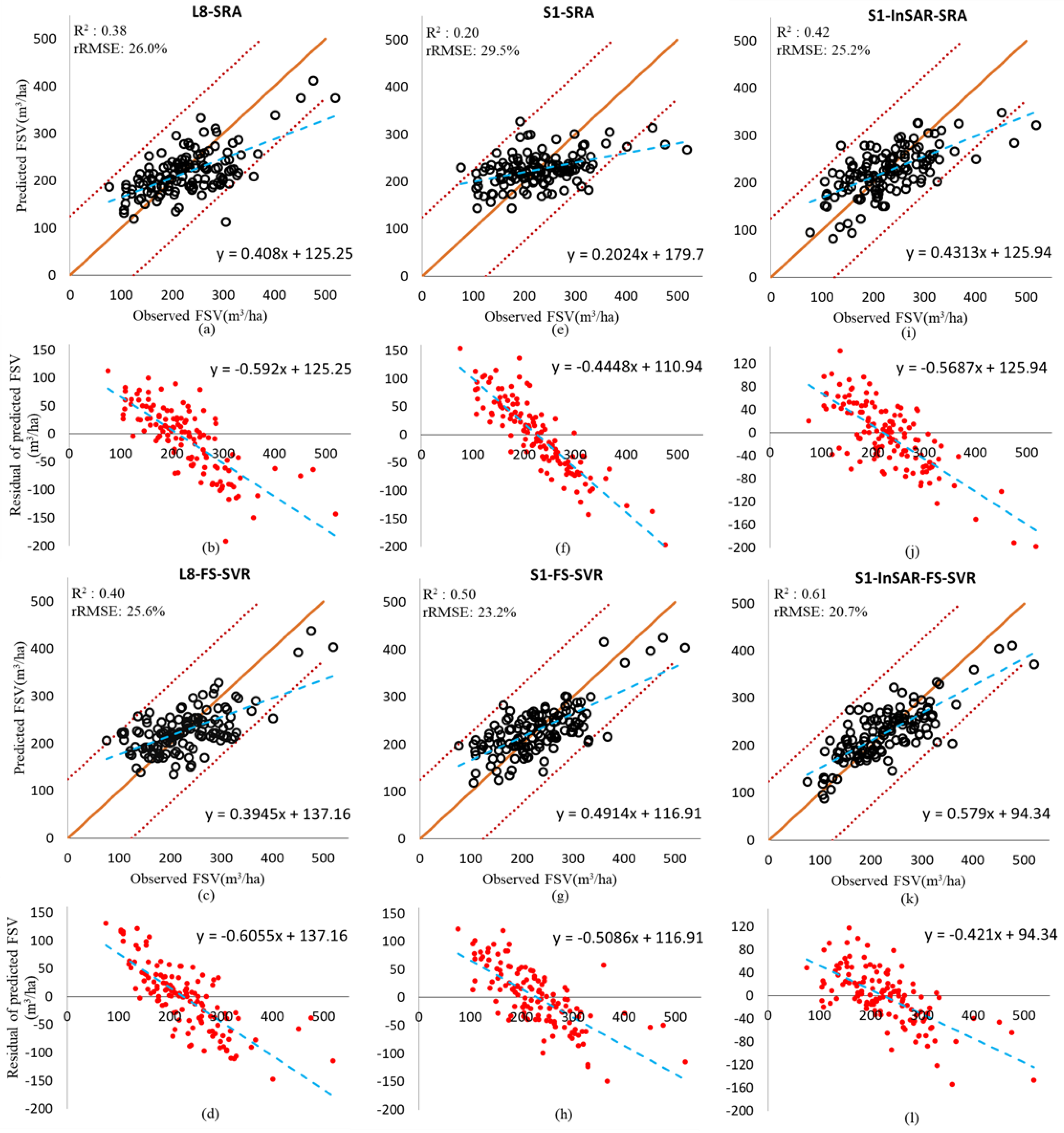
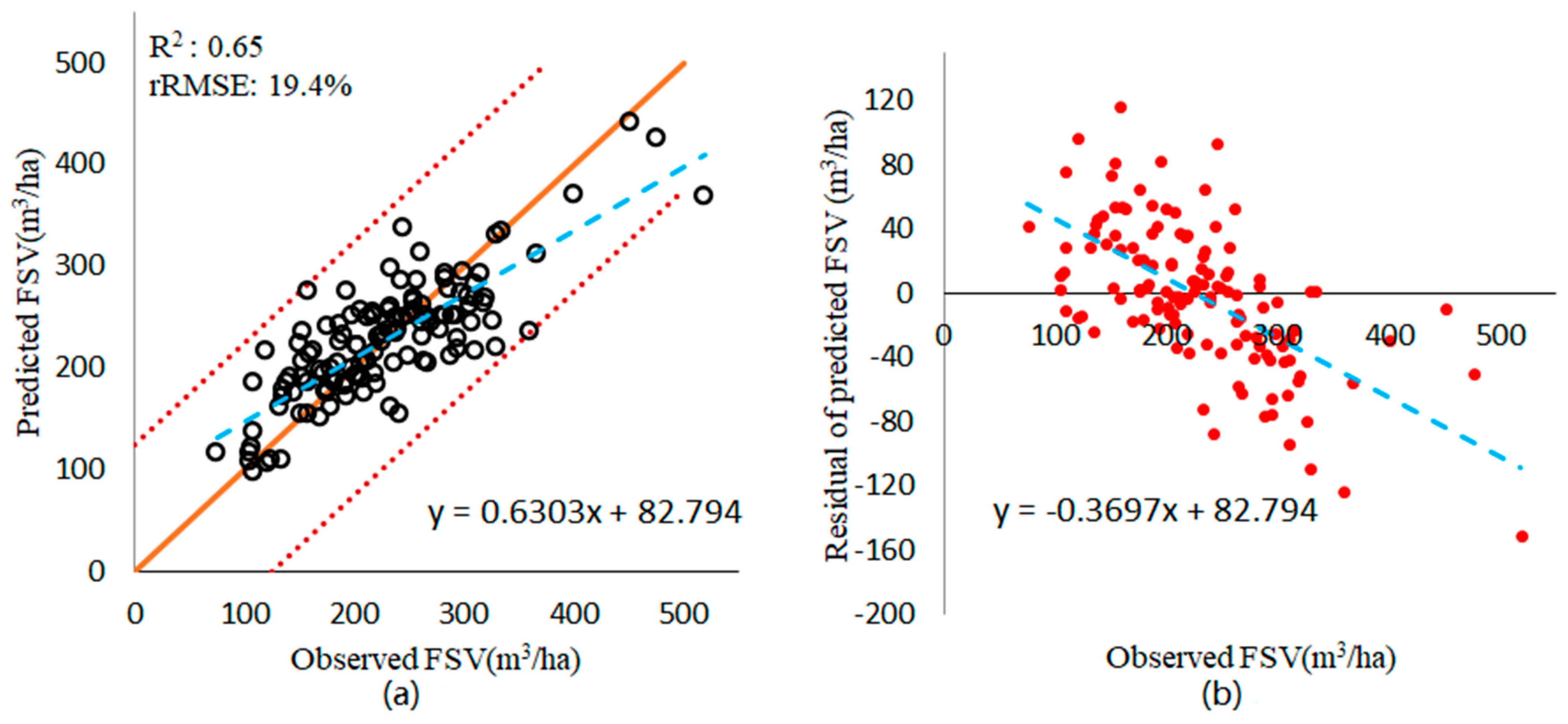
4.2. FSV Prediction Result

Using the SVR linear kernel function and RBF kernel function algorithm, the coniferous forest stock volume estimation model of the Wangyedian Forest Farm was constructed based on the subset of feature variables selected by the SRA and FS-SVR methods (Figure 5). The prediction accuracies corresponding to the three datasets, L8, S1, and S1-InSAR, are listed in

Table 9. Hyperparameter sets and prediction accuracies of support vector regression constructed by the SRA and FS-SVR methods.

Datasets	Methods	C	Gamma	R2	RMSE (m3/ha)	rRMSE (%)	r
L8	SRA	100		0.38	59.0	25.9	0.63
	FS-SVR	150	2.8	0.40	58.4	25.6	0.63
S1	SRA	200		0.20	67.3	29.5	0.45
	FS-SVR	350	1.4	0.50	52.9	23.2	0.71
S1-InSAR	SRA	51		0.42	57.3	25.2	0.65
	FS-SVR	150	4.8	0.61	47.2	20.7	0.78
The integrated dataset	FS-SVR	270	2.4	0.65	44.3	19.4	0.81

Note: The integrated dataset, the combination of L8, S1, and S1-InSAR datasets; r, Pearson correlation between FSV estimates and observations.

. In general, the S1-InSAR dataset had a better estimation performance for coniferous forest stock volume than that of S1 and L8. The combination of feature variables selected by the FS-SVR method is more suitable for coniferous FSV estimation than those selected by the SRA method. The average value of rRMSE obtained by FSV estimation based on the three datasets using the FS-SVR method was 23.17%, which was 13.8% lower than the average value of rRMSE corresponding to the SRA method (26.87%). When the SRA method was used, the FSV estimation performance of S1-InSAR and L8 was significantly higher than that of the S1 dataset, and the corresponding rRMSE values were 14.6% and 12.2% lower than that of S1, respectively, which also verified the correlation analysis results in Table 5, Table 6 and Table 7. For the FS-SVR method, the S1-InSAR feature factor set obtained by interferometry yielded good FSV estimation performance. The R², RMSE, and rRMSE values were 0.61, 47.2 m³/ha, and 20.7%, respectively. To explore the synergistic potential of active and passive remote sensing combined data in northern coniferous forest stock volume estimation, we integrated the L8, S1, and S1-InSAR datasets and conducted FSV estimation experiments based on the FS-SVR method. The results show that the integrated dataset can provide full play to the synergy of the three remote sensing datasets (Figure 6). There was a strong correlation between the forest stock volume predicted values and observed values; the PC coefficient (r) value reached 0.81, and the RMSE and rRMSE values were 44.3 m³/ha and 19.4%, respectively.

By using the FS-SVR method, the subset of feature variables selected based on the integrated dataset of L8, S1, and S1-InSAR and its estimation performance change trends are shown in Figure 7. The feature variables that contribute the most to the estimation accuracy of forest stock volume were InSAR coherence factors, followed by S1 backscattering texture factors and L8 OLI vegetation indices. With an increase in the number of feature variables, the estimation accuracy of the forest stock volume exhibits an obvious upward trend. Particularly notable is that, when the interference coherence factors 1202VV-CC and 0617VV-CC were added to the set of feature variables, the estimation accuracies (1-rRMSE) were 8.8% and 5.7% higher than those before the addition, respectively. The contribution of backscattering coefficient texture factor 0921VH-S-W9T3 to the improvement of forest stock volume estimation accuracy was relatively smaller than that of the feature factor related to VV polarization, which further verified the conclusion in Section 4.1; that is, the forest stock volume correlation of S1 VV polarization is higher than that of VH polarization.

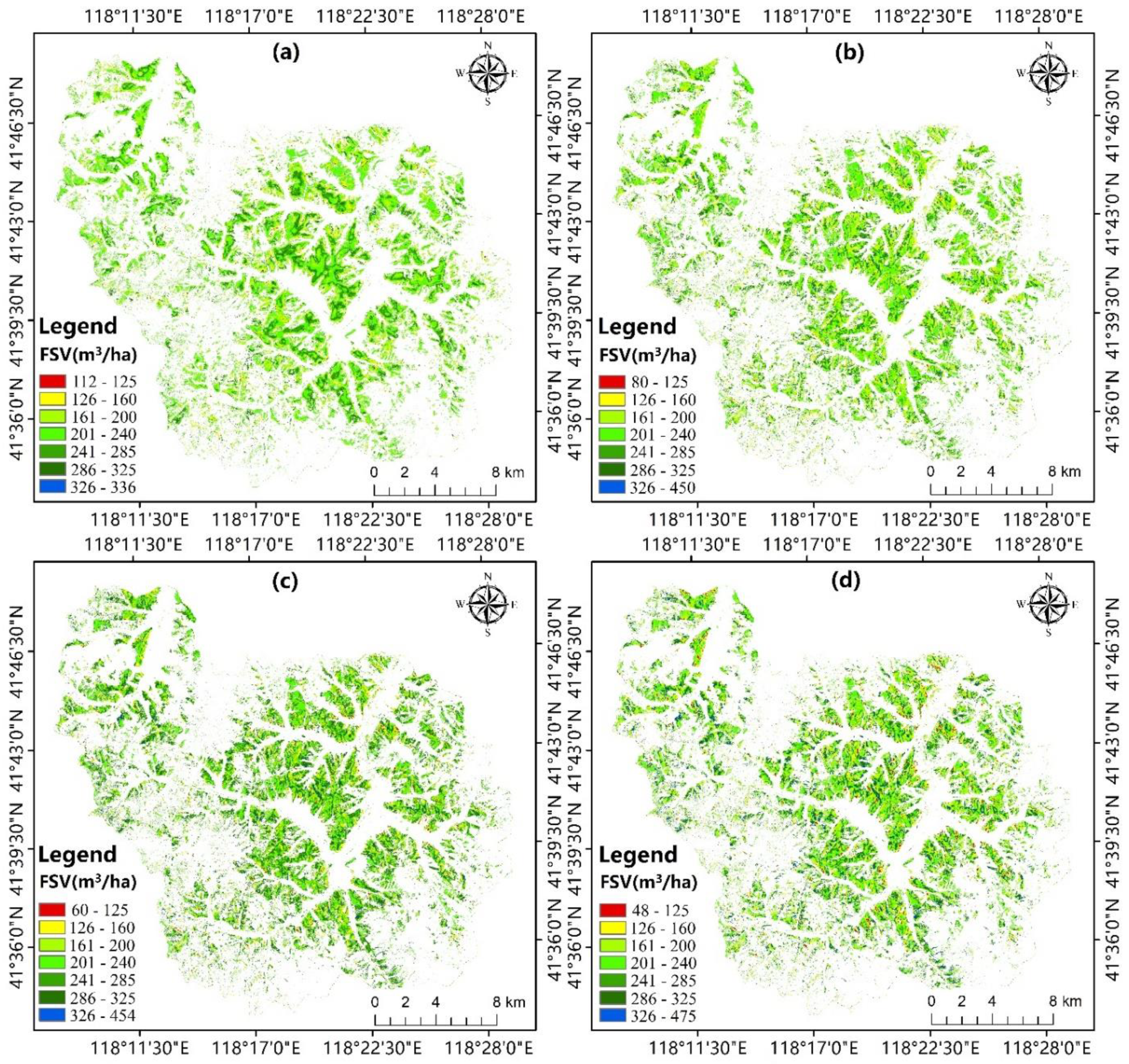
4.3. Predicting and Mapping the Stock Volume of Coniferous Plantation

To compare and analyze the stock volume estimation performance of different remote sensing datasets in the Wangyedian coniferous forest, we performed forest stock volume prediction and spatial distribution mapping based on the L8, S1, and S1-InSAR datasets (Figure 8a–c). The distribution range of the FSV estimates in Figure 8a was 112–336 m³/ha, the low value of FSV was concentrated around 130 m³/ha, and the high value was mainly concentrated around 300 m³/ha, indicating that there were serious problems due to low-value overestimation and high-value underestimation, which also verified that the L8 image dataset suffers from a low saturation point in regions with high FSV values, resulting in very limited estimation capabilities. Figure 8b,c have larger FSV distribution ranges than Figure 8a, and their estimation results are also more accurate than those in Figure 8a. Especially in Figure 8c, the prediction effect in the low- and high-value areas of the FSV was significantly improved, and it was more in line with the actual FSV distribution than Figure 8a,b. The aforementioned results show that the S1-InSAR dataset can effectively improve the estimation accuracy and saturation of the FSV in the Wangyedian coniferous forest.

This study, using the integrated dataset of L8, S1, and S1-InSAR, combined with the sample data of the coniferous FSV in the study area, constructed an FSV estimation model using the FS-SVR method and an SVR algorithm. The coniferous FSV in the Wangyedian study area was predicted, and an FSV spatial distribution inversion map with 30 m resolution was generated (Figure 8d). The coniferous FSVs of the Wangyedian research area in 2019 ranged from 48 to 475 m³/ha, most of which were below 325 m³/ha, and the average value and standard deviation were 201 m³/ha and 62 m³/ha, respectively, which is consistent with the statistical results of our sampling survey. The low-value areas of coniferous FSV were concentrated in the central and northern low-altitude areas with many of human activities, and the high-value areas of the coniferous FSV were located in the relatively high-altitude or sparsely populated remote forest areas in the east and west, away from cities and towns.

5. Discussion

5.1. Feature Variables Selection in FSV Estimation

Unlike the SRA method, which focuses on selecting characteristic variables with good linear correlation, the FS-SVR method can measure the nonlinear relationship between feature variables, and FSV and considers the combination optimization effect between features. Therefore, the PC values of the feature variables in Table 8 were generally lower than those in Table 5, Table 6 and Table 7. However, the statistics of the FSV estimation results in Table 9 and Figure 5 demonstrate that the FS-SVR method proposed in this study has better FSV estimation accuracy than the SRA method does. Especially with respect to the FSV estimation based on the S1 dataset, the R² and fitting trendline slope corresponding to the FS-SVR method were 150.0% and 142.8% higher than those of the SRA method, respectively. These results also show that the combination effect between the feature variables is a crucial factor that cannot be ignored in the process of feature variable selection [12,50]. In addition, the correlation and importance statistics results in Table 7 and Table 8 demonstrate that the VV polarization of the S1 image is significantly better than that of the VH polarization. In a study of forest AGB estimation based on optical and SAR remote sensing data in Dunhua City, Jilin Province, China, Chen [61] found that Sentinel-1 was more sensitive to forest AGB under VV polarization data than HH polarization was. This finding is consistent with the results of this study.

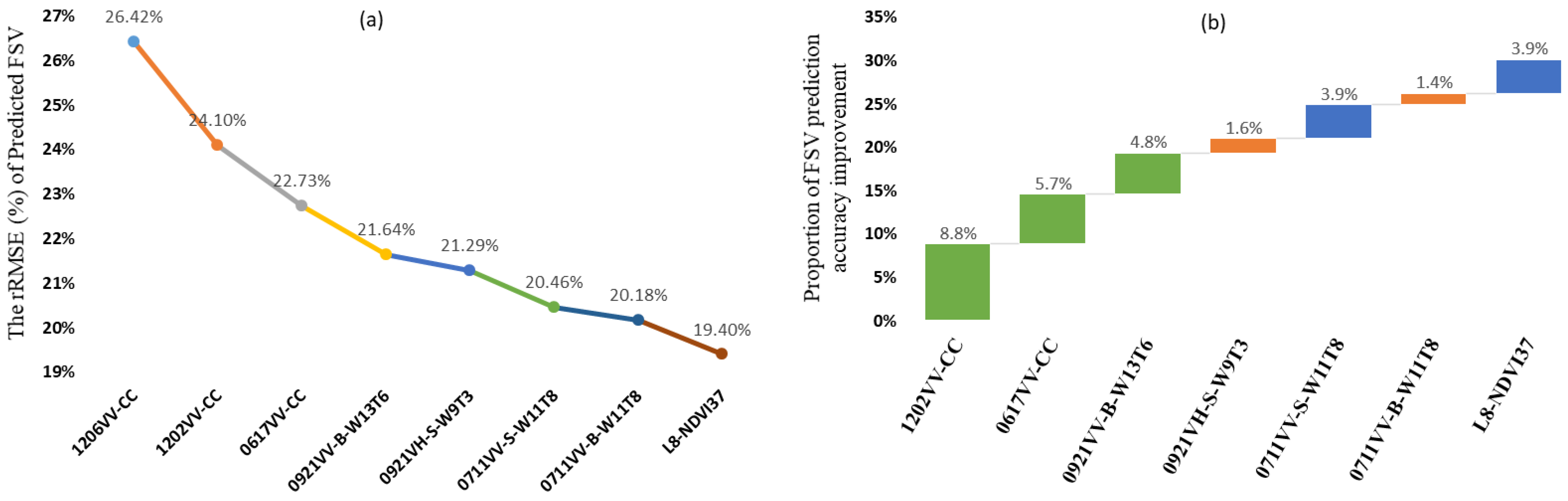
5.2. Analysis of FSV Estimation Performance

We compared the estimation results of the FSV model in Figure 5 and Figure 6 and found that the fitting effect of the model corresponding to the integrated dataset was the best, the slope of the fitting trendline (0.63) was the highest, and the fitting trendline of the FSV estimation residual value was the flattest. This finding shows that the synergy of the three remote sensing datasets can effectively suppress the problems of high-value underestimation and low-value overestimation in FSV estimation. The statistical results in Figure 7 demonstrate that the feature variable with the greatest improvement in the estimation accuracy of FSV in the three datasets is the S1-InSAR coherence coefficient, which may be because the coherent amplitude data contain the vertical structure information related to the forest canopy height. Therefore, the S1-InSAR dataset has a better FSV response and higher saturation point than the S1 backscattering coefficient and optical remote sensing factors do. Borlafmena et al. [45] tested the ability of the Sentinel-1 C-band image to distinguish forests from other land-use types and found that InSAR coherence feature factors can improve overall classification accuracy. Robert et al. [55] systematically evaluated the potential of Sentinel-1, Sentinel-2, and Landsat 8 for use in permanent grassland moving event detection. The results showed that comprehensive prediction accuracy based on the combined data of NDVI, the backscattering coefficient, and InSAR coherence was the highest. The findings of the aforementioned research are very similar to the conclusions of this study, which prove the great potential of the Sentinel-1 C-band and its InSAR coherence feature factors with respect to remote sensing classification and quantitative estimation.

Tomáš et al. [62] extracted radar polarization coherent amplitude data and optical remote sensing variables based on Sentinel-1 and Sentinel-2 data, supplemented by a sample survey and airborne laser scanning data, and established an AGB prediction model that used multiple regression. The best model RMSE was 41.2 t/ha, and the rRMSE was 35.1%. Long et al. [39] estimated the FSV of the Chinese fir plantation in South China by using Alos-2 PALSAR L-band full polarimetric SAR data. They found that the fused polarimetric features based on a timeseries of SAR images can improve the estimation accuracy of FSV, and the minimum rRMSE was 24.42%. In the aforementioned two studies, the difficulty of performing remote sensing prediction on forest AGB in reference [62] is essentially equivalent to that of the FSV estimation in this study. The Chinese fir forest studied in reference [39] is a coniferous plantation that contains larches and Chinese pines, similar to this study, but the FSV estimation accuracy (1-rRMSE) obtained in our study is 24.2% and 6.6% higher than those of the other two studies, respectively. The main reason for the above results is that we extracted many InSAR coherent amplitude factors based on hyper-temporal Sentinel-1 images, which improved the diversity of the remote sensing feature variables. In addition, we used the FS-SVR method to optimize the selection process of the feature variables.

5.3. Limitations and Prospects

There are many uncertain factors in the process of FSV remote sensing estimation that affect estimation accuracy, such as ground sample data, satellite sensor images, and feature variables for modeling [10,52]. The ground sample plots selected by sampling are representative. Too few sample plots cannot fully and accurately describe the actual distribution and law of the FSV [20]. Therefore, to minimize the errors caused by sampling, this study integrated field sample plot survey data from 2017 and 2019. There are some differences in the FSV saturation and estimation performance of different satellite sensor data. This study found that the estimated saturation point of L8 was approximately 300 m³/ha, and the estimated maximum FSV value in the study area was 336 m³/hal; whereas the saturation point of the S1-InSAR dataset was approximately 390 m³/ha, the estimated maximum FSV value in the study area was 454 m³/ha, and the best RMSE was 47.6 m³/ha. The aforementioned results are mainly because the optical sensor signal cannot penetrate the dense forest canopy, resulting in the spectral signal tending to be saturated [18,20]. After interference processing of the S1 image results, the coherence coefficient and DSM data containing canopy height information can be obtained [42]. These S1-InSAR feature factors significantly improved the saturation and accuracy of FSV estimation. Because the interferometric coherence effect of the S1 images in the same period as the field survey is often not guaranteed, it is necessary to perform interferometric processing based on S1 hyper-temporal images to improve the diversity and effectiveness of coherent amplitude data. Such processing requires considerable time, and relying solely on InSAR technology cannot directly obtain tree height information in mountain forests [61]. ICESat-2 (Ice, Cloud, and Land Elevation Satellite-2) is a spaceborne LiDAR satellite that was launched in September 2018 [25]. Research [25,26] shows that ICESat-2 can obtain a large-scale forest vegetation canopy height. Therefore, for exploring effective solutions to further improve the accuracy of FSV remote sensing estimation, follow-up research can use ICESat2 data, combined with S1-InSAR and other optical remote sensing data, to synergistically retrieve the FSV. In addition, related research has used environmental factors, such as land surface temperature and soil moisture retrieved from Landsat 8 thermal infrared sensor images, to conduct remote sensing estimation and the modeling of parameters such as forest AGB and leaf area index [20,53,63]. However, the validity of environmental factors such as land surface temperature, soil moisture, and topographic moisture for estimating coniferous FSV has not been verified.

The set of remote sensing feature variables used to construct the FSV estimation model can significantly affect the final prediction results [10]. Pearson, SRA, and other linear relationship measurement methods can simply and quickly select feature variables linearly related to FSV. However, forests are characterized by spatial heterogeneity and dynamic changes. This method, based on linear correlation, cannot comprehensively and accurately describe the real relationship between the FSV and remote sensing variables in a complex forest environment [12]. In addition, the RF feature selection method can only screen the relatively crucial feature factors based on specific evaluation criteria, without considering the combination effect relationship between feature factors, which may be able to be coupled with other factors to some extent; thus, it has the potential to improve the accuracy of FSV estimation [50]. Compared with the SRA method, the FS-SVR method proposed in this paper has significant advantages in the FSV estimation of Wangyedian coniferous forests but needs to be verified in FSV research on other forest types in other research areas, and the operation efficiency of the algorithm needs to be improved. Nonparametric models represented by machine learning algorithms usually have better FSV estimation performance than parametric models do in a complex forest environment [10,50]. In this study, the estimation accuracy of the SVR model based on the RBF kernel function was higher than that based on the linear kernel function. However, due to the spatial heterogeneity of forest ecosystems, there remains a certain estimation error in the FSV estimated by the SVR model (rRMSE, 19.4%). The hybrid model, combining the parametric or nonparametric model and the residual Kriging interpolation model, showed excellent performance in forest AGB estimation [61], and the RMSE reached 29.72 Mg/ha. In further research, a Kriging interpolation model based on geostatistics can be considered for FSV prediction research.

6. Conclusions

In this study, L8 OLI multispectral images, C-band S1, and interferometric radar data were used to extract various remote sensing feature factors, and an improved method for the selection of remote sensing feature variables (FS-SVR) was explored. On the basis of three datasets and the SVR model, a FSV remote sensing estimation experiment on coniferous forest was conducted, and an FSV estimation scheme, combined with active and passive multisource remote sensing data, was proposed. Finally, spatial distribution inversion mapping of the coniferous FSV in the Wangyedian Forest Farm was conducted.

The conclusions of this study are as follows: (1) The S1-InSAR dataset generated based on S1 hyper-temporal image interferometry had good FSV estimation accuracy. The R² reached 0.6, the RMSE value was 47.6 m³/ha, and the rRMSE value was 20.9%. Because the coherent amplitude and DSM data contain the vertical structure information related to the forest canopy height, and the hyper-temporal S1 image data greatly enriches the diversity of S1-InSAR feature factors, they have a better FSV response and a higher saturation point than remote sensing factors do, such as the S1 backscattering coefficient and the L8 vegetation index. (2) The integrated dataset of L8, S1, and S1-InSAR can fully play the synergy of the three remote sensing datasets. The RMSE and rRMSE values are 44.3 m³/ha and 19.4%, respectively. There is a strong correlation between the FSV predicted value and observed value, and r reaches 0.81, which is 28.6%, 14.1%, and 3.8% higher than those of L8, S1, and S1-InSAR, respectively. The feature variables that contribute the most to the accuracy of FSV estimation in the integrated dataset are InSAR coherence factors, followed by S1 backscattering coefficient texture factors and L8 vegetation indices. The backscattering coefficient and the InSAR feature factor of the VV polarization in the S1 image provide better FSV estimation performance than the VH polarization. (3) The proposed FS-SVR method is very suitable for the selection of remote sensing features in FSV estimation. The average value of rRMSE (23.17%) obtained using the FS-SVR method for FSV estimation based on the three datasets was 13.8% lower than that of the SRA method (26.87%). This study helps realize the high-precision estimation and mapping of regional forest volumes by collecting a small amount of measured forest plot data combined with global coverage, free-download multispectral images (Landsat 8), and C-band SAR data (Sentinel-1), which have practical theoretical guidance and practical demonstration significance for the development of remote sensing estimation technology for regional forest volumes, and will promote the further improvement of modern forestry resources management.

References

1. Sun, W.; Liu, X. Review on carbon storage estimation of forest ecosystem and applications in China. For. Ecosyst. 2020, 7, 37–50. [Google Scholar] [CrossRef] [Green Version]
2. Ali, F.; Khan, N.; Abd_Allah, E.; Ahmad, A. Species Diversity, Growing Stock Variables and Carbon Mitigation Potential in the Phytocoenosis of Monotheca buxifolia Forests along Altitudinal Gradient across Pakistan. Appl. Sci. 2022, 12, 1292. [Google Scholar] [CrossRef]
3. Yan, W.; Wang, W.; Peng, Y.; Chen, X. Evaluation of Biomass and Carbon Stocks in Three Pine Forest Types in Karst Area of Southwestern China. J. Sustain. For. 2022, 41, 18–32. [Google Scholar] [CrossRef]
4. Sasaki, N.; Myint, Y.; Abe, I.; Venkatappa, M. Predicting carbon emissions, emissions reductions, and carbon removal due to deforestation and plantation forests in Southeast Asia. J. Clean. Prod. 2021, 312, 127728. [Google Scholar] [CrossRef]
5. Zhao, J.; Zhao, L.; Chen, E.; Li, Z.; Xu, K.; Ding, X. An Improved Generalized Hierarchical Estimation Framework with Geostatistics for Mapping Forest Parameters and Its Uncertainty: A Case Study of Forest Canopy Height. Remote Sens. 2022, 14, 568. [Google Scholar] [CrossRef]
6. Gschwantner, T.; Alberdi, I.; Bauwens, S.; Bender, S.; Borota, D.; Bosela, M.; Bouriaud, O.; Breidenbach, J.; Donis, J.; Fischer, C.; et al. Growing stock monitoring by European National Forest Inventories: Historical origins, current methods and harmonisation. For. Ecol. Manag. 2022, 505, 119868. [Google Scholar] [CrossRef]
7. Rees, W.G.; Tomaney, J.; Tutubalina, O.; Zharko, V.; Bartalev, S. Estimation of Boreal Forest Growing Stock Volume in Russia from Sentinel-2 MSI and Land Cover Classification. Remote Sens. 2021, 13, 4483. [Google Scholar] [CrossRef]
8. Persson, H.J. Estimation of Boreal Forest Attributes from Very High Resolution Pléiades Data. Remote Sens. 2016, 8, 736. [Google Scholar] [CrossRef] [Green Version]
9. Astola, H.; Hame, T.; Sirro, L.; Molinier, M.; Kilpi, J. Comparison of Sentinel-2 and Landsat 8 imagery for forest variable prediction in boreal region. Remote Sens. Environ. 2019, 223, 257–273. [Google Scholar] [CrossRef]
10. Li, X.; Liu, Z.; Lin, H.; Wang, G.; Sun, H.; Long, J.; Zhang, M. Estimating the growing stem volume of Chinese Pine and Larch Plantations based on fused optical data using an improved variable screening method and stacking algorithm. Remote Sens. 2020, 12, 871. [Google Scholar] [CrossRef] [Green Version]
11. Fassnacht, F.E.; Hartig, F.; Latifi, H.; Berger, C.; Hernández, J.; Corvalán, P.; Koch, B. Importance of sample size, data type and prediction method for remote sensing-based estimations of aboveground forest biomass. Remote Sens. Environ. 2014, 154, 102–114. [Google Scholar] [CrossRef]
12. Li, X.; Lin, H.; Long, J.; Xu, X. Mapping the Growing Stem Volume of the Coniferous Plantations in North China Using Multispectral Data from Integrated GF-2 and Sentinel-2 Images and an Optimized Feature Variable Selection Method. Remote Sens. 2021, 13, 2740. [Google Scholar] [CrossRef]
13. Rutishauser, E.; Wrigh, S.; Condit, R.; Hubbell, S.; Davies, S.; Muller-Landau, H.C. Testing for changes in biomass dynamics in large-scale forest datasets. Glob. Change Biol. 2020, 26, 1485–1498. [Google Scholar] [CrossRef] [PubMed]
14. Sebastian, W.; Christian, H.; Mikhail, K.; Christiane, S. Large Area Mapping of Boreal Growing Stock Volume on an Annual and Multi-Temporal Level Using PALSAR L-Band Backscatter Mosaics. Forests 2014, 5, 1999–2015. [Google Scholar] [CrossRef] [Green Version]
15. Zhang, Y.; Liang, S. Fusion of Multiple Gridded Biomass Datasets for Generating a Global Forest Aboveground Biomass Map. Remote Sens. 2020, 12, 2559. [Google Scholar] [CrossRef]
16. Lindberg, E.; Hollaus, M. Comparison of methods for estimation of stem volume, stem number and basal area from airborne laser scanning data in a hemi-boreal forest. Remote Sens. 2012, 4, 1004–1023. [Google Scholar] [CrossRef] [Green Version]
17. Wijaya, A.; Kusnadi, S.; Gloaguen, R.; Heilmeier, H. Improved strategy for estimating stem volume and forest biomass using moderate resolution remote sensing data and GIS. J. For. Res. Jpn. 2010, 21, 1–12. [Google Scholar] [CrossRef]
18. Zhao, P.; Lu, D.; Wang, G.; Wu, C.; Huang, Y.; Yu, S. Examining spectral reflectance saturation in Landsat imagery and corresponding solutions to improve forest aboveground biomass estimation. Remote Sens. 2016, 8, 469. [Google Scholar] [CrossRef] [Green Version]
19. Bogan, S.A.; Antonarakis, A.S.; Moorcroft, P.R. Imaging spectrometry-derived estimates of regional ecosystem composition for the Sierra Nevada, California. Remote Sens. Environ. 2019, 228, 14–30. [Google Scholar] [CrossRef]
20. Lu, D.; Chen, Q.; Wang, G.; Li, G.; Moran, E. A survey of remote sensing-basedd aboveground biomass estimation methods in forest ecosystems. Int. J. Digit. Earth 2016, 9, 63–105. [Google Scholar] [CrossRef]
21. Puliti, S.; Saarela, S.; Gobakken, T.; Stahl, G.; Naesset, E. Combining UAV and Sentinel-2 auxiliary data for forest growing stock volume estimation through hierarchical model-based inference. Remote Sens. Environ. 2018, 204, 485–497. [Google Scholar] [CrossRef]
22. Bilous, A.; Myroniuk, V.; Holiaka, D.; Bilous, S.; See, L.; Schepaschenko, D. Mapping growing stock volume and forest live biomass: A case study of the Polissya region of Ukraine. Environ. Res. Lett. 2017, 12, 105001. [Google Scholar] [CrossRef] [Green Version]
23. Chrysafis, I.; Mallinis, G.; Gitas, I.; Tsakiri-Strati, M. Estimating Mediterranean forest parameters using multi seasonal Landsat 8 OLI imagery and an ensemble learning method. Remote Sens. Environ. 2017, 199, 154–166. [Google Scholar] [CrossRef]
24. García-Gutiérrez, J.; Martínez-álvarez, F.; Troncoso, A.; Riquelme, J.C. A comparison of machine learning regression techniques for lidar-derived estimation of forest variables. Neurocomputing 2015, 167, 24–31. [Google Scholar] [CrossRef]
25. Neuenschwander, A.L.; Magruder, L.A. Canopy and terrain height retrievals with ICESat-2: A first look. Remote Sens. 2019, 11, 1721. [Google Scholar] [CrossRef] [Green Version]
26. Narine, L.L.; Popescu, S.; Neuenschwander, A.; Zhou, T.; Srinivasan, S. Estimating aboveground biomass and forest canopy cover with simulated ICESat-2 data. Remote Sens. Environ. 2019, 224, 1–11. [Google Scholar] [CrossRef]
27. Fu, L.; Liu, Q.; Sun, H.; Wang, S.; Li, Z.; Chen, E.; Pang, Y.; Song, X.; Wang, G. Development of a system of compatible individual tree diameter and aboveground biomass prediction models using error-in-variable regression and airborne LiDAR data. Remote Sens. 2018, 10, 325. [Google Scholar] [CrossRef] [Green Version]
28. Chen, Q.; Laurin, G.V.; Battles, J.J.; Saah, D. Integration of airborne LiDAR and vegetation types derived from aerial photography for mapping aboveground live biomass. Remote Sens. Environ. 2012, 121, 108–117. [Google Scholar] [CrossRef]
29. Zhang, Y.; Shao, Z.F. Assessing of urban vegetation biomass in combination with LiDAR and high-resolution remote sensing images. Int. J. Remote Sens. 2021, 42, 964–985. [Google Scholar] [CrossRef]
30. Cao, L.; Coops, N.C.; Innes, J.L.; Sheppard, S.R.J.; Fu, L.; Ruan, H.; She, G. Estimation of forest biomass dynamics in subtropical forests using multi-temporal airborne LiDAR data. Remote Sens. Environ. 2016, 178, 158–171. [Google Scholar] [CrossRef]
31. Sinha, S.; Jeganathan, C.; Sharma, L.K.; Nathawat, M.S. A review of radar remote sensing for biomass estimation. Int. J. Environ. Sci. Technol. 2015, 12, 1779–1792. [Google Scholar] [CrossRef] [Green Version]
32. Soja, M.J.; Quegan, S.; D’Alessandro, M.M.; Banda, F.; Scipal, K.; Tebaldini, S.; Ulander, L.M.H. Mapping above-ground biomass in tropical forests with ground-cancelled P-band SAR and limited reference data. Remote Sens. Environ. 2021, 253, 112153. [Google Scholar] [CrossRef]
33. Vafaei, S.; Soosani, J.; Adeli, K.; Fadaei, H.; Naghavi, H.; Pham, T.D.; Bui, D.T. Improving accuracy estimation of forest aboveground biomass based on incorporation of ALOS-2 PALSAR-2 and Sentinel-2A imagery and machine learning: A case study of the Hyrcanian Forest area (Iran). Remote Sens. 2018, 10, 172. [Google Scholar] [CrossRef] [Green Version]
34. Kumar, L.; Mutanga, O. Remote sensing of above-ground biomass. Remote Sens. 2017, 9, 935. [Google Scholar] [CrossRef] [Green Version]
35. Cai, Y.; Li, X.; Zhang, M.; Lin, H. Mapping wetland using the object-based stacked generalization method based on multi-temporal optical and SAR data. Int. J. Appl. Earth Obs. Geoinf. 2020, 92, 102164. [Google Scholar] [CrossRef]
36. Santoro, M.; Beaudoin, A.; Beer, C.; Cartus, O.; Fransson, J.E.S.; Hall, R.J.; Pathe, C.; Schmullius, C.; Schepaschenko, D.; Shvidenko, A. Forest growing stock volume of the northern hemisphere: Spatially explicit estimates for 2010 derived from Envisat ASAR. Remote Sens. Environ. 2015, 168, 316–334. [Google Scholar] [CrossRef]
37. Zhu, Y.; Liu, K.; Myint, S.W.; Du, Z.; Wu, Z. Integration of GF2 Optical, GF3 SAR, and UAV Data for Estimating Aboveground Biomass of China’s Largest Artificially Planted Mangroves. Remote Sens. 2020, 12, 2039. [Google Scholar] [CrossRef]
38. Zhao, Q.; Yu, S.; Zhao, F.; Tian, L.; Zhao, Z. Comparison of machine learning algorithms for forest parameter estimations and application for forest quality assessments. For. Ecol. Manag. 2019, 434, 224–234. [Google Scholar] [CrossRef]
39. Long, J.; Lin, H.; Wang, G.; Sun, H.; Yan, E. Estimating the growing stem volume of the planted forest using the general linear model and time series quad-polarimetric sar images. Sensors 2020, 20, 3957. [Google Scholar] [CrossRef]
40. Purohit, S.; Aggarwal, S.P.; Patel, N.R. Estimation of forest aboveground biomass using combination of Landsat 8 and Sentinel-1A data with random forest regression algorithm in Himalayan Foothills. Trop. Ecol. 2021, 62, 288–300. [Google Scholar] [CrossRef]
41. Liu, G.; Zbigniew, P.; Stefano, S.; Benni, T.; Wu, L.; Fan, J.; Bai, S.; Wei, L.; Yan, S.; Song, R.; et al. Land Surface Displacement Geohazards Monitoring Using Multi-temporal InSAR Techniques. J. Geod. Geoinf. Sci. 2021, 4, 77–87. [Google Scholar] [CrossRef]
42. Chen, L.; Wang, Y.; Ren, C.; Zhang, B.; Wang, Z. Assessment of multi-wavelength SAR and multispectral instrument data for forest aboveground biomass mapping using random forest kriging. For. Ecol. Manag. 2019, 447, 12–25. [Google Scholar] [CrossRef]
43. Tomppo, E.; Antropov, O.; Praks, J. Boreal Forest Snow Damage Mapping Using Multi-Temporal Sentinel-1 Data. Remote Sens. 2019, 11, 384. [Google Scholar] [CrossRef] [Green Version]
44. Tanase, M.A.; BorlafMena, I.; Santoro, M.; Aponte, C.; Marin, G.; Apostol, B.; Badea, O. Growing Stock Volume Retrieval from Single and Multi-Frequency Radar Backscatter. Forests 2021, 12, 944. [Google Scholar] [CrossRef]
45. BorlafMena, I.; Badea, O.; Tanase, M.A. Assessing the Utility of Sentinel-1 Coherence Time Series for Temperate and Tropical Forest Mapping. Remote Sens. 2021, 13, 4814. [Google Scholar] [CrossRef]
46. Zhang, R.; Xiang, W.; Liu, G.; Wang, X.; Mao, W.; Fu, Y.; Cai, J.; Zhang, B. Interferometric coherence and seasonal deformation characteristics analysis of saline soil based on Sentinel-1A time series imagery. J. Syst. Eng. Electron. 2021, 32, 1270–1283. [Google Scholar] [CrossRef]
47. Jänichen, J.; Schmullius, C.; Baade, J.; Last, K.; Bettzieche, V.; Dubois, C. Monitoring of Radial Deformations of a Gravity Dam Using Sentinel-1 Persistent Scatterer Interferometry. Remote Sens. 2022, 14, 1112. [Google Scholar] [CrossRef]
48. Tong, X.; Xu, X.; Chen, S. Coseismic Slip Model of the 2021 Maduo Earthquake, China from Sentinel-1 InSAR Observation. Remote Sens. 2022, 14, 436. [Google Scholar] [CrossRef]
49. Dai, K.; Xu, Q.; Li, Z.; Tomás, R.; Fan, X.; Dong, X.; Li, W.; Zhou, Z.; Gou, J.; Ran, P. Post-disaster assessment of 2017 catastrophic Xinmo landslide (China) by spaceborne SAR interferometry. Landslides 2019, 16, 1189–1199. [Google Scholar] [CrossRef] [Green Version]
50. Li, X.; Long, J.; Zhang, M.; Liu, Z.; Lin, H. Coniferous Plantations Growing Stock Volume Estimation Using Advanced Remote Sensing Algorithms and Various Fused Data. Remote Sens. 2021, 13, 3468. [Google Scholar] [CrossRef]
51. Luo, M.; Wang, Y.; Xie, Y.; Zhou, L.; Qiao, J.; Qiu, S.; Sun, Y. Combination of feature selection and catboost for prediction: The first application to the estimation of aboveground biomass. Forests 2021, 12, 216. [Google Scholar] [CrossRef]
52. Li, X.; Zhang, M.; Long, J.; Lin, H. A Novel Method for Estimating Spatial Distribution of Forest Above-Ground Biomass Based on Multispectral Fusion Data and Ensemble Learning Algorithm. Remote Sens. 2021, 13, 3910. [Google Scholar] [CrossRef]
53. Jiang, F.; Kutia, M.; Ma, K.; Chen, S.; Long, J.; Sun, H. Estimating the aboveground biomass of coniferous forest in Northeast China using spectral variables, land surface temperature and soil moisture. Sci. Total Environ. 2021, 785, 147335. [Google Scholar] [CrossRef] [PubMed]
54. Zhang, Y.; Ma, J.; Liang, S.; Li, X.; Li, M. An evaluation of eight machine learning regression algorithms for forest aboveground biomass estimation from multiple satellite data products. Remote Sens. 2020, 12, 4015. [Google Scholar] [CrossRef]
55. Lobert, F.; Holtgrave, A.-K.; Schwieder, M.; Pause, M.; Vogt, J.; Gocht, A.; Erasmi, S. Mowing event detection in permanent grasslands: Systematic evaluation of input features from Sentinel-1, Sentinel-2, and Landsat 8 time series. Remote Sens. Environ. 2021, 267, 112751. [Google Scholar] [CrossRef]
56. Doyog, N.D.; Lin, C.; Lee, Y.J.; Lumbres, R.I.C.; Daipan, B.P.O.; Bayer, D.C.; Parian, C.P. Diagnosing pristine pine forest development through pansharpened-surface-reflectance Landsat image derived aboveground biomass productivity. For. Ecol. Manag. 2021, 487, 119011. [Google Scholar] [CrossRef]
57. Chrysafis, I.; Mallinis, G.; Siachalou, S.; Patias, P. Assessing the relationships between growing stock volume and Sentinel-2 imagery in a Mediterranean forest ecosystem. Remote Sens. Lett. 2017, 8, 508–517. [Google Scholar] [CrossRef]
58. Granero-Belinchon, C.; Adeline, K.; Briottet, X. Impact of the number of dates and their sampling on a NDVI time series reconstruction methodology to monitor urban trees with Venμs satellite. Int. J. Appl. Earth Obs. Geoinf. 2021, 95, 102257. [Google Scholar] [CrossRef]
59. Sarker, M.; Nichol, J.; Iz, H.B.; Ahmad, B.B. Forest biomass estimation using texture measurements of high-resolution dual-polarization C-band SAR data. IEEE Trans. Geosci. Remote Sens. 2013, 51, 3371–3384. [Google Scholar] [CrossRef]
60. Wang, J.; Wu, F.; Shang, J.; Zhou, Q.; Ahmad, I.; Zhou, G. Saline soil moisture mapping using Sentinel-1A synthetic aperture radar data and machine learning algorithms in humid region of China’s east coast. Catena 2022, 213, 106189. [Google Scholar] [CrossRef]
61. Chen, L. Modeling of Forest Aboveground Biomass Based on Optical and Interferometric Synthetic Aperture Radar. Ph.D Thesis, University of Chinese Academy of Sciences, Beijing, China, 2020. [Google Scholar] [CrossRef]
62. Bucha, T.; Papčo, J.; Sačkov, I.; Pajtík, J.; Sedliak, M.; Barka, I.; Feranec, J. Woody Above-Ground Biomass Estimation on Abandoned Agriculture Land Using Sentinel-1 and Sentinel-2 Data. Remote Sens. 2021, 13, 2488. [Google Scholar] [CrossRef]
63. Dube, T.; Mutanga, O. The impact of integrating WorldView-2 sensor and environmental variables in estimating plantation forest species aboveground biomass and carbon stocks in uMgeni Catchment, South Africa. ISPRS J. Photogramm. Remote Sens. 2016, 119, 415–425. [Google Scholar] [CrossRef]
Figure 1. (a) Study area location; (b) Landsat 8 image of the study area; (c) Sentinel-1 C-band SAR image of the study area.
Remotesensing 14 02754 g001
Figure 2. (a) Plot distribution map and digital elevation model (DEM) of the study area; (b) distribution of coniferous forest, other forest types, and non-forest land in the study area; (ce) images of larches and Chinese pines at the field survey sites, respectively.
Remotesensing 14 02754 g002
Figure 3. Flow chart of interference processing based on Sentinel-1 IW SLC images.
Remotesensing 14 02754 g003
Figure 4. Some intermediate results obtained by radar interferometry based on Sentinel-1 images.
Remotesensing 14 02754 g004
Figure 5. Scatterplots of FSV prediction results using L8 (ad), S1 (eh), and S1-InSAR (il) datasets, respectively. (a,b,e,f,i,j) SRA variable selection method. (c,d,g,h,k,l) FS-SVR variable selection method. The red dotted line is the 50% error bar, used to judge whether the error of the FSV estimated value exceeds 50% of the sample mean; the orange solid line is the 1:1 diagonal line; and the blue dotted line is the linear fitting trendline. The formula is the linear equation fitted by the scatterplot.
Remotesensing 14 02754 g005
Figure 6. (a) Scatterplots of FSV prediction results based on integrated dataset of L8, S1, and S1-InSAR using the FS-SVR feature variable selection method and support vector regression model. (b) Residual distribution of FSV predicted value. The formula is the linear equation fitted by the scatterplot.
Remotesensing 14 02754 g006
Figure 7. (a) FSV prediction rRMSE change trend with the increase in feature variables; (b) improvement trend of FSV prediction accuracy (1-rRMSE).
Remotesensing 14 02754 g007
Figure 8. FSV distribution maps of coniferous plantations in the study area based on the FS-SVR method, using four remote sensing datasets. (a) L8, (b) S1, (c) S1-InSAR, (d) the integrated of three datasets.
Remotesensing 14 02754 g008