Article

Hyperspectral Reflectance Proxies to Diagnose In-Field Fusarium Head Blight in Wheat with Machine Learning

1
National Engineering and Technology Center for Information Agriculture, Key Laboratory for Crop System Analysis and Decision Making, Ministry of Agriculture, Jiangsu Key Laboratory for Information Agriculture, Jiangsu Collaborative Innovation Center for Modern Crop Production, Nanjing Agricultural University, Nanjing 210095, China
2
National Key Laboratory of Crop Genetics and Germplasm Enhancement, Cytogenetics Institute, Nanjing Agricultural University, Nanjing 210095, China
*
Authors to whom correspondence should be addressed.
Remote Sens. 2022, 14(12), 2784; https://doi.org/10.3390/rs14122784
Submission received: 3 May 2022 / Revised: 3 June 2022 / Accepted: 6 June 2022 / Published: 10 June 2022
(This article belongs to the Special Issue Crop Biophysical Parameters Retrieval Using Remote Sensing Data)

Abstract

:
Hyperspectral reflectance (HR) technology as proxy approach to diagnose fusarium head blight (FHB) in wheat crop could be a real-time and non-invasive approach for its in-field management to reduce grain damage. In-field canopy’s non-imaging HR (400–2400 nm using ground-based spectrometer system), photosynthesis rate (Pn) and disease severity (DS) data were simultaneously acquired from artificially inoculated wheat plots over a period of two years (2020 and 2021) in the field. Subsequently, continuous wavelet transform (CWT) was employed to select the consistent spectral bands (CSBs) and to develop the canopy-based difference indices with criterion of variable importance score using random forest—recursive feature elimination. Thereby, different machine learning algorithms were employed for FHB classification and multivariate estimation, and linear regression models to evaluate the newly developed indices against conventional vegetation indices. The results showed that inoculation reduced the Pn rate of spikes, elevated reflectance in visible and short-wave infrared regions and decreased in near infrared region at different days after inoculation (DAI). CWT analysis selected five CSBs (401, 460, 570, 786 and 840 nm) employing datasets from 2020 and 2021. These spectral bands were employed to develop wheat fusarium canopy indices (WFCI1 and WFCI2). Considering the average classification accuracy (ACA) in both years of experiments, WFCI1 manifested a maximum ACA of 75% at 5 DAI with DS of 9.73% which raised to 100% at 10 DAI with a DS of 18%. ACA mentions the averaged results of all machine learning classifiers (MLC). While in the perspective of MLC, random forest (RF) outperformed the rest of the MLC, individually, it revealed 100% classification accuracy through WFCI1 at DS 10.78% on the eight DAI. The univariate estimation of disease based on WFCI1 and WFCI2 with independent data produced R2 and root mean square error (RMSE) values of 0.80 and 14.7, and 0.81 and13.50, respectively. However, Knn regression analysis with both canopy indices (WFCI1 and WFCI2) manifested the maximum accuracy for disease estimation with RMSE of 11.61 and R2 = 0.83. Conclusively, the newly proposed HR indices show great potential as proxy approach for detecting FHB at early stage and understanding the physical state of crops in field conditions for the better management and control of plant diseases.

1. Introduction

Fusarium head blight (FHB), caused by Fusarium graminearum Schwabe, is one of the main diseases that negatively impact wheat production [1]. The Yangtze River and Huai River basin in China is a hotbed of FHB, and there have been reports of the disease in the Yellow River basin and it is slowly making its way north [2]. Resultantly, toxins—deoxynivalenol and zearalenone—can be produced, which can be harmful to animals and humans and lead to food safety issues when FHB-infected wheat is harvested [3]. For this reason, it is critical to accurately identify FHB in order to prevent and control the disease.
Wheat FHB has been identified using a variety of methods. Visual monitoring has traditionally been used to determine the prevalence of wheat FHB in the field. However, this approach requires a significant investment of time and effort. Furthermore, it is susceptible to the influence of one’s own subjective consciousness. It is possible to see changes in wheat’s spectral reflectance caused by fungus infection in the morphology and internal physiological structure of infected plant tissues [3,4,5]. Given these, hyperspectral imaging (HSI) has been used by many researchers to identify FHB in wheat ears. According to Zhang et al. [6], the HSI of wheat ears was used to develop a special FHB classification index that could be successfully used to classify wheat HSI data. The successful classification of healthy and infected wheat spikes was achieved using the convolutional neural network classification algorithm applied to HSI pixels. Using HSI to detect wheat ears has made significant progress [7,8,9]. HSI, on the other hand, requires a substantial increase in computing resources (memory and bandwidth) [10]. Alternatively, non-imaging spectrometers can detect crop spectral information at a lower cost and faster speed than HSI, reducing data processing time. However, it does not contain spatial information [11].
Non-imaging or hyperspectral (HR) instruments have been used by several researchers to detect wheat FHB. In order to establish a wheat FHB identification model with an overall accuracy of more than 88%, a ground surface spectrometer to measure the spectra from the wheat ears [11]. Huang et al. [12] used a spectrometer to measure wheat ears and extracted derivative and absorption features and vegetation indices (VIs). Afterward, they used these features to build effective disease severity (DS) identification models under the combination of Fisher’s linear discriminant analysis and support vector machine (SVM). For the identification of FHB in wheat ears, HR technology has great potential. However, a limited number of studies have studied FHB at spike scale and canopy scale. HR sensing has not yet been practiced in a time series manner to the best of our knowledge.
Plant diseases can be monitored at different scales, from individual leaf to fields and regional scales, using hyperspectral remote sensing (RS) [4]. Certain disease symptoms can complicate canopy-scale hyperspectral signatures based on canopy structure and crop morphology [13,14]. Using hyperspectral RS for crop disease monitoring requires the selection of spectral features that can measure disease in terms of both quantity and quality, regardless of the canopy structures. Plant’s water deficiency and chlorophyll loss can be caused by various plant diseases [15]. It is possible that a diseased plant’s spectral reflectance may have different characteristics at the water and/or chlorophyll absorption bands than healthy plants [14]. The ability of canopy-scale spectral features and sensing methods to detect these different signatures of infection in the field should be evaluated. To better understand how different spectral features can detect disease at an early infection level and quantify crop DS, this study will be particularly useful. Accordingly, the identification of sensitive bands or spectral features susceptible to crop disease classification and detection using hyperspectral data is critical.
Several scientists have demonstrated that RS is a reliable alternative for the noninvasive monitoring of plant stress conditions and growth parameters with VIs [16,17,18]. These can be used as a proxy approach to quantify crop DS and physiological changes under disease stress. Disease-specific hyperspectral VIs improve the ability to diagnose plant diseases by utilizing hyperspectral observations that enable the characterization of subtle differences in plants and crop canopies in comparison to conventional VIs [15,19]. For example, hyperspectral DS indices have been developed specifically for the purpose of monitoring wheat leaf rust [20]. Different plant diseases can also produce disease-specific spectral signatures, which can be used to distinguish between them in the field [19]. As a result, it is critical to understand which spectral vegetation index (VI) has the greatest ability to provide an accurate measure of crop DS.
Thus, an FHB disease-specific approach is needed for its diagnosis. Hence, the primary goal of this study was to develop a spectroscopic approach that could be used to distinguish between healthy and FHB-infected wheat canopies at various days after inoculation (DAI) and disease severities (DS). Specifically, we sought to perform the following: (1) monitor canopy’s photosynthetic response to FHB infection; (2) to determine the sets of consistent spectral features using appropriate wavelet-based selected bands; (3) to develop normalized difference FHB spectral indices and compare them with conventional vegetation indices; (4) canopy scale disease estimation through univariate and multivariate regression modeling; and, finally, (5) to evaluate the comparative classification performance of different machine learning algorithms.

2. Materials and Methods

2.1. Experiment Detail

2.1.1. Study Site and Plant Material

Two consecutive field experiments were conducted on winter wheat in Jiangsu province, China. The first experiment (2020) was conducted from 2 November 2019 to 18 June 2020 and the second (2021) from 14 November 2020 to 16 June 2021 in Qinhuai District, Nanjing (32°1′N, 118°15′E), at the Pailou experimental base of Nanjing Agricultural University.
The wheat cultivars, Aikang-58 as susceptible and Sumai-3 as resistant, were grown to measure the dynamic spectral response of the wheat canopy under the infection of the FHB. The experiments were repeated in the same field by using a randomized complete block design with six replications (Figure 1A) for each treatment (healthy and diseased) and cultivar. The dimension of each plot was 6 m2 (3 m × 2 m), growing wheat seeds with a line-to-line distance of 25 cm. The wheat plots were tap watered if needed and fertilized at the recommended dose, using urea CO(NH2)2 for Nitrogen (N)—225 kg/ha; calcium superphosphate Ca (H2PO4)2 for phosphorus (P2O5)—125 kg/ha; and potassium chloride (KCL) for potassium—120 kg/ha. All fertilizers were applied as basal dose except N, which was split into two doses and half as a basal dose, and the remaining was applied at the jointing stage through top-dressing. A continuous wheat crop monitoring was established for crop health (weeding, irrigation, fungicide and insecticide application) until the start of the emergence of the wheat spikes. To be noted, there were no applications of fungicide and insecticide after the start of the emergence of wheat ears.

2.1.2. Disease Inoculation and Description of Disease Severity Scaling

For canopy scale disease inoculation, half of the plots (Figure 1A-top) were inoculated with prepared spores’ suspension of 50 mL for each plot. The inoculum was sprayed very carefully on spikes at the flowering stage or Zadok’s growth stage 61–66; after spraying, almost 200 spikes were covered with zipper bags for 12 h to retain high humidity for the successful inoculation of FHB. The inoculation was made in the afternoon and to make sure successful inoculation was obtained, we inoculated around 100 spikes by using injection methods, which were feasible for inoculation by standing at the border of the plot without damaging wheat plants or disturbing canopy’s stand. All inoculation operations were completed at the same day. For the first experiment (2020), inoculation was made on 16 April 2020 and for the second experiment (2021), inoculation was made on 11 April 2021.
The DS of the canopy was observed by counting the number of infected spikelets to the total number of spikelets by visual observation. We measured the canopy’s DS using the methodology of Luedeling et al. [21,22]. Ten locations were selected (Ten-points sampling) on a permanent basis in each plot, and from each location, ten spikes were marked with the color marker at the stem (below three leaves). The samples (spikes) percentage was calculated by counting the number of spikelets [22]. Around 100 spikes were examined by abandoning the border area of each plot from where spectral measurements were supposed to be performed. For each plot, the DS was calculated by employing Equation (1):
DS % = 3 %   × n 1 + 5 % × n 2 + 10 %   × n 3 100 %   × n 9 n 0 + n 1 + n 3 + n 9 × 100
where DS is the scale of the disease severity, n1, n2, ……, n9 are the number of spikes at different disease severities and n0 denotes the number of healthy spikes.

2.2. Data Acquisition

2.2.1. Field Reflectance Data Acquisition

The canopy scale reflectance was measured using Analytical Spectral Devices (ASD) that was operated by holding its probe optical fiber in a handheld pistol (an accessory) to measure canopy reflectance at a sampling interval of 1.4 nm in the 350–1000 nm region and 1.1 nm in the 1001–2500 nm span. A fiber-optic contact cable (1.5 m) paired with FieldSpec 4 array detector was used to catch the light reflected from the target. In both years of the experiments, canopy reflectance was measured from two points in each plot, which were marked and consistently measured throughout the experiment. On the other hand, the measured point and DS reading points were kept common. The data were always acquired from 10:00 h to 14:00 h (Beijing time) at noon with clear sunshine and low airwaves. The distance between the pistol and canopy was kept at almost 1 m height with 25° field of view and uniform for all plots, while a white reflectance panel (Standard) was also fixed at the level of canopy height using an adjustable tripod (Figure 1B). ASD was optimized after the measurement of each three plots. After the average of acquired 30 spectral signatures on each measurement day from each plot was obtained, a total of 3 spectra were retained and used for subsequent analysis for both years of experiments (2020 and 2021).

2.2.2. Photosynthesis Rate (Pn)

The canopy’s photosynthesis (Pn) was measured using a newly developed P-Chamber (Figure 1C) integrated with LI-6400XT (LI-6400, Lincoln, NE, USA), a portable photosynthesis gadget. The P-Chamber of size 30 cm × 5 cm × 5 cm (L × W × H) is equipped with double-sided red and blue LED light source and operates in a wide range of temperature (0–50 °C) and humidity (0–95%) without condensation. The CO2 flow rate was maintained at 800 due to the large size of the P-chamber. Further in-depth detail can be found at [email protected] and Chang et al. [23]. For canopy, 25 labeled spikes from each plot were measured.

2.3. Data Analysis Interpretation

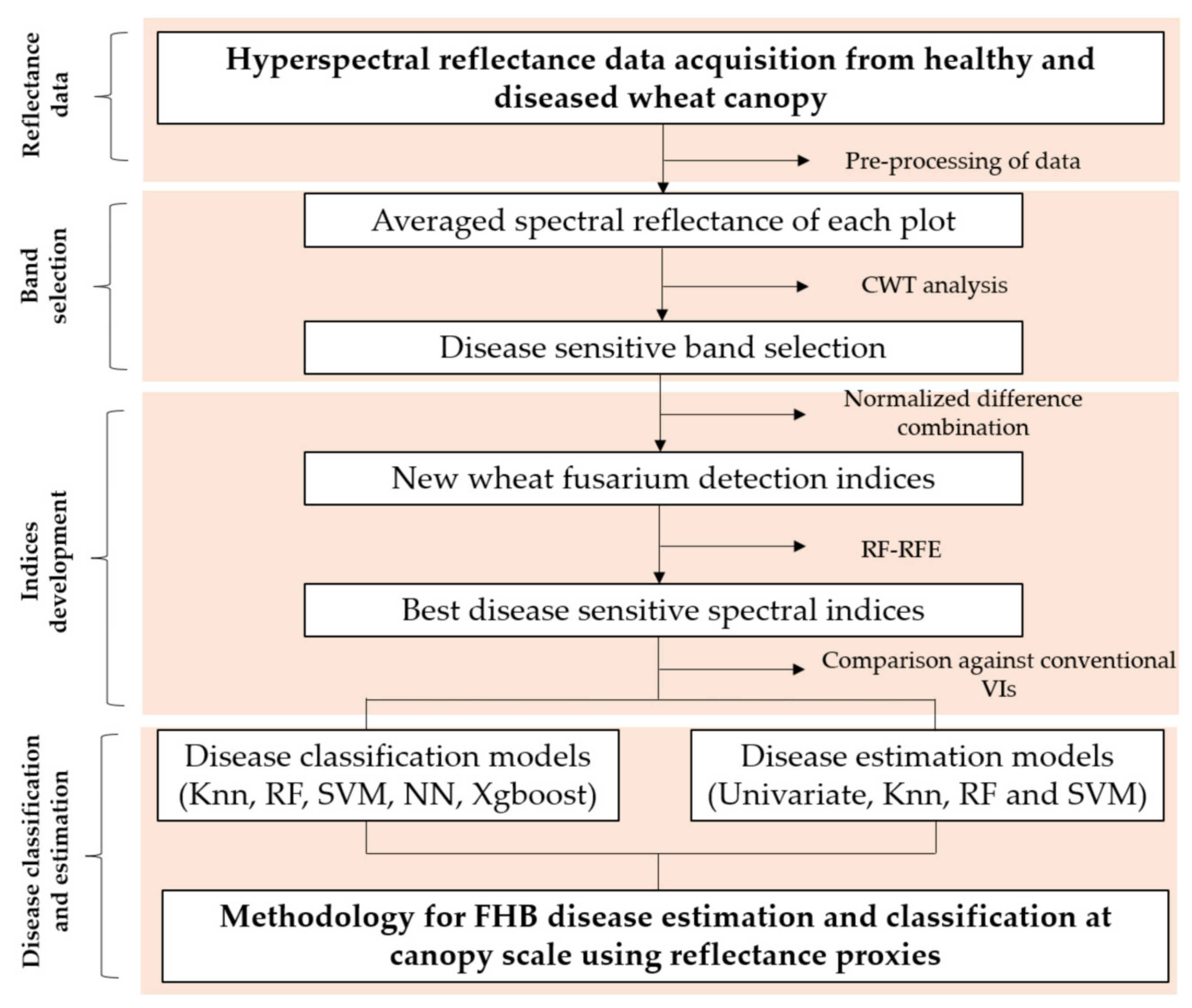
The FHB detection and estimation study with consistent features are divided into six segments: (1) selection of spectral features by continuous wavelet transform (CWT); (2) development of normalized spectral indices imputing CSBs; (3) selection of best canopy indices using random forest—recursive feature elimination (RF-RFE); (4) selection of consistent conventional vegetation indices; (5) classification through machine learning classifiers (MLC) such as i. K nearest neighbors (Knn), ii. support vector machine (SVM), random forest (RF), neural net (NN) and extreme gradient boost (Xgboost); (6) univariate disease estimation modeling; and (7) multivariate disease estimation, such as i. RF regression (RFR), ii. SVM regression (SVMR) and iii. Knn regression (KnnR). Figure 2 illustrates the flow of the study and data analysis methodology.

2.3.1. Methodology to Feature Selection and Indices Development

Hyperspectral datasets are commonly used, and they encompass a bunch of variables. This large volume of data can limit software’s handling ability. This increase in information may be useful for the classification process but it increases the number of variables that can cause a “dimensionality curse” [24]. RS studies use feature selection (FS), which is a representative subset of variables. The most sensitive features are selected according to the objected problem. Numerous studies have practiced similar approaches, but most of them fed the pooled dataset to select features instead of considering the severity proportion or period of the problem and were classified between treated and controlled [4,20]. However, very few studies [25,26] explored the consistent behavior of the consistent sensitive features based on severity proportion. We selected the consistent spectral bands (CSBs) to develop indices. For CSBs, datasets of 2020 (9 and 16 DAI) and 2021 (10 and 19 DAI) were used because minimum and moderate DS (11 to 30%) are currently considered to be alike, and also a study have used 30% DS for plant disease indices development [19].

Selection of Consistent Spectral Features by Continuous Wavelet Transform (CWT)

Wavelets analyses have shown vigorous potential for hyperspectral signal processing in reducing the dimensionality curse by performing discrete wavelet transform (DWT) and CWT [27]. Regarding plant studies, CWT is commonly used due to its comparable output coefficients with original reflectance signal [26]. On the contrary, DWT results output coefficients that are not interpretable with the face of original spectra; hence, it causes interpretation difficulty. Many recent plant stress studies [25,26] successfully applied CWT and selected the spectral features on the basis of wavelet scales, which showed very high classification accuracy (CA). Therefore, we imputed CWT in our study for reflectance band selection from non-imaging spectrometer data. The following steps explain the CWT-based bands selection.
(a) Continuous wavelets transformation: This is the basic process of the CWT, which permutes original spectrum signals into coefficient sets through mother wavelet-based function at different scales and wavelengths. The scaling and shifting of mother wavelets ψ(λ) produces wavelets ψa,b(λ) in transformation [28]:
ψ a , b λ = 1 a ψ λ b a
where a is scaling factor and it represents wavelet width, and b as shifting factor represents the position.
(b) Wavelet power scalogram: The output power coefficients from original spectrum are explained by following equation.
w f a , b = f , ψ a , b = + f λ ψ a , b λ d λ
Given any fixed scale ai (i = 1,2, …, m, m is fully available scale), any waveband can shift continuous wavelets and the CWT of a spectrum generates vector (1 × n) of wavelet coefficients. In Equation (3), f(λ) is number of wavebands (λ = 1, 2, …n); for this study, the reflectance spectrum consists of n = 236 (nm). The coefficient sets (Wf (ai,bj), i = 1, 2, …, m, j = 1, 2, …, n), shape two dimensional scalogram: One shows scale and the other represents waveband (m × n matrix). It is the wavelet power that is represented by each individual element of a scalogram, and it measures the correlation between a segment of the reflectance spectrum. Moreover, it measures the scaled and shifted mother wavelet, as well as the similarity of specific spectral shape to a certain wavelet basis. Low-scale portions of the scalogram contain absorption features with precise spectral details, while high-scale components replicate the general continuum of the reflectance spectrum, and both types of components are used in conjunction with each other. Since the canopy’s spectra (400–2400 nm) absorption features are identical in shape with Gaussian or quasi-Gaussian functions, therefore, Gaussian’s second derivative—named as Mexican Hat—was selected as basis for mother wavelet. The possible continuum scales (i = 1, 2, …, m) of wavelet incur time and storage. Therefore, the dimensions of scalogram can be reduced by decomposing the spectra into dyadic scales (21, 22, 23, …, and 210 labeled in this study as scale 1, scale 2 and so on), which are in relation to the length of the wavelet compressed or stretched at that scale [29]. We engaged scales 0 to 8 for feature extraction.
(c) Disease correlation scalogram: After basic CWT and considering 2–8 scales, the coefficient of determinant (R2) analysis between disease severities and wavelet coefficients for different disease scales provides a correlation scalogram in the form of matrix (m × n). We can identify highly disease sensitive wavelet features from this scalogram.
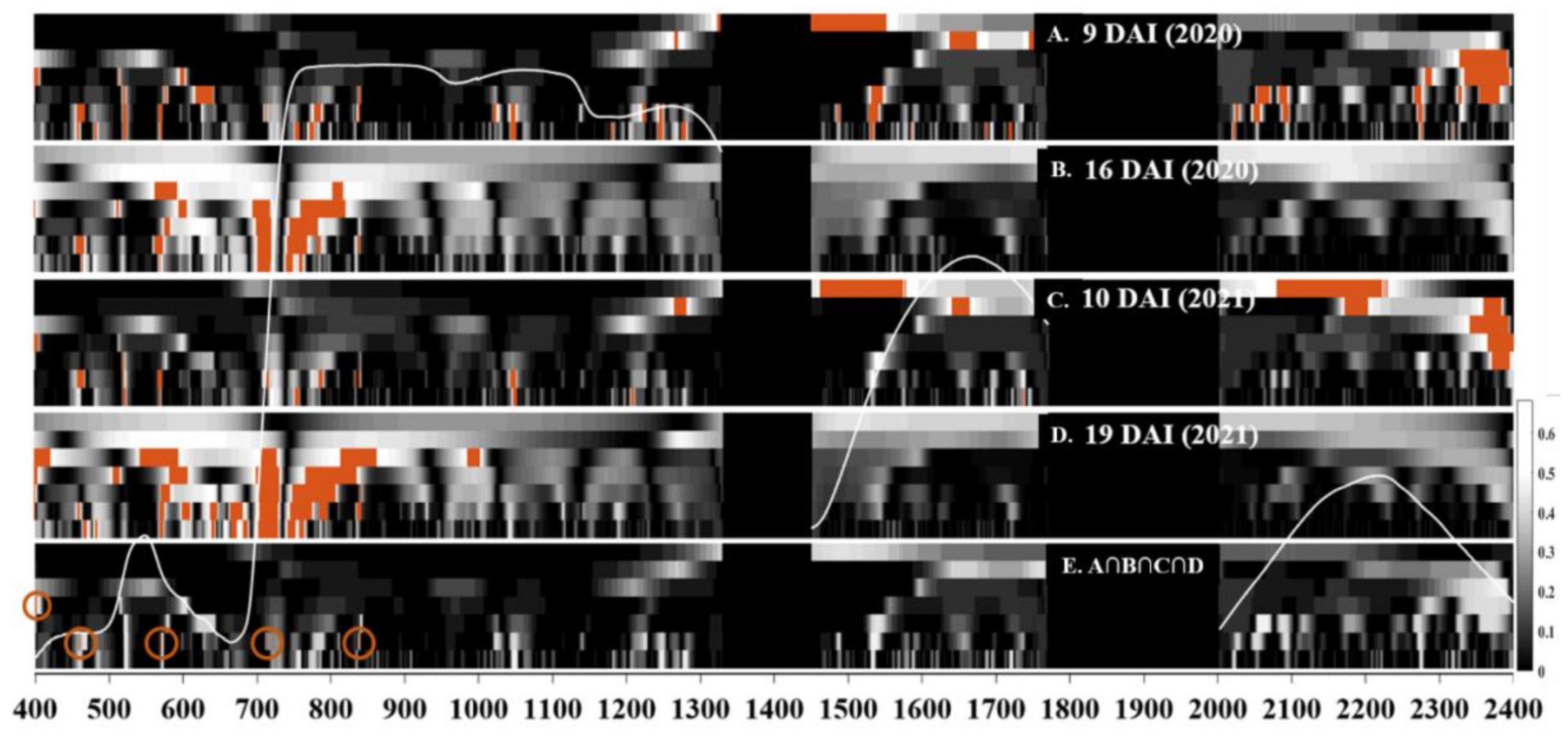
(d) Thresholding and intersection to identify wavelet features: The highly sensitive wavelet features were extracted through thresholding from aforementioned scalogram. For this study, at each DAI, we highlighted uppermost 5% elements showing R2 values; thereafter, intersection was taken among individual years’ correlation scalogram, highlighting red regions. At last, the intersection was taken to select consistent wavelet features for all correlation scalograms. Selected CSBs were consistent for both years but from lower DS which in combination represents total 28% DS.

Development of Spectral Indices

The disease-specific wheat fusarium canopy indices (WFCI) were developed independently in accordance with previous studies [4,13]. For spectral indices development, we computed normalized difference indices, including five CSBs. Each CSB was named as F1 or F2, and was calculated using following expression.
WFCI = F 1 F 2 F 1 + F 2
The computed difference indices were screened out on the basis of variable importance score (VIP) score by RF-RFE. The spectral features and texture features were calculated independently.
RF is an embedded algorithm, and it entails the qualities of both the filter and wrapper methods. On the other hand, RFE is a wrapper method. RF-RFE is combination of both, and further details can be found in study Gregorutti et al. [30]. RF-RFE works on recursive phenomenon, which grades the features according to their importance. Firstly, the dataset was divided into train and test sets. Secondly, RF classifier ranks each feature on the basis of its importance and eliminates unnecessary features in each iteration. Thus, a subset of features was obtained. Lastly, RFE tests the subset of variables in stepwise recursive manner and reordered the features on the basis of their classification performance.

2.3.2. Selection of Consistent Vegetation Indices

We also evaluated the consistent behavior of 92 conventional VIs of eight categories (Table S3) of all datasets to figure out which indices are more sensitive to FHB and compared them against newly developed indices [19]. Instead of using categorized disease scales, we computed a pooled dataset of each year (2019–2020 and 2020–2021) individually for all indices. The statistical filter method was used for variable selection, and correlation (R) was applied to calculate the degree of correlation. Subsequently, among top 8 VIs of each year, common indices were selected as consistent indices [25] for FHB investigation and comparison against newly developed indices.

2.3.3. Machine Learning Algorithms

Machine learning classifiers (MLC) are inevitable for hyperspectral datasets and have showed remarkable performance in several studies. However, occasionally, their performance fluctuates due to uncertain explanations relevant to data issue (e.g., unbalance, missing, size and type of data). MLC’s basic functions include sensor type, scale or location and computing efficiency [31]. Therefore, to overcome all possibilities and validating selected features’ performance, we proposed and developed five MLC to make intra-comparisons and quantitively discriminate healthy against diseased spikes. Among them, four (Knn, RF, SVM and NN) are widely used but the fifth one, Xgboost, has yet to be practiced for plant diseases. All MLC were computed using different packages in “R environment” where the seed (1234) and data partitions (Train—70%—and test—30%) were kept the same for all classifiers and disease scale datasets. On the other hand, performance was measured through the attributes of the confusion matrix, and the results are presented as Accuracy Equation (5) [32]. It is noted that we practiced supervised binary classification:
Accuracy = TP + TN TP + TN + FP + FN
where TP is actually infected and the model also predicted this state, TN is predicted to be the same in an actual healthy model, FP is actually healthy but the model predicted it as infected and FN is actually infected but the model predicted it to be healthy.
K Nearest Neighbor (Knn) is a straightforward non-parametric classifier in machine learning (ML). It works on nearest neighbor phenomenon and affiliates the test sample to specific category depending on the k value. On the other hand, the k value is calculated by different distance functions, such as Hamming, Minkowski, Manhattan and Euclidean. We used Minkowski distances due to the continuous nature of variables [33]. Support vector machine (SVM) is a linear function, and it is highly tested and an efficient non-parametric ML algorithm for high dimensional and small dataset problems. Generically, SVM was developed for two-class classification. We applied radial basis function using the LibSVM library [34]. Random forest (RF) is a decision trees-based ensembled ML classifier that randomly selects the training (n) samples by replacement to construct each decision tree. A detailed description can be observed in Belgiu and Drăguţ [35]. A neural network (NN) is a non-linear black box of interconnected neurons that is used as a ML classifier. Following the activation of the function, each input gains a weighting value, which is then used at the summation junction to produce an output signal on the basis of the acquired value. Further details can be found in [36]. In this study, we developed the NN model with one hidden layer and 300 epochs and validated using the repeated cross-validation approach. Xgboost (Extreme Gradient Boost): In 2016, Chen and Guestrin [37] proposed this machine learning decision tree ensembled method based on a gradient boost algorithm. A new tree is trained in each iteration to enhance the performance of pre-existing tree to improve classification.
The separability efficiencies of all MLCs were measured by a confusion matrix—Equation (5). We performed all MLC in an R environment (Version 4.0.1) using “Knn” [38], “randomforest” [39], “e1071” [40], “nnet” [41] and “Xgboost” [42] packages for Knn, RF, SVM, NN and Xgboost, respectively.

2.3.4. Statistical Analysis of Canopy Photosynthesis and Disease Estimation

The linear correlation of all biochemical parameters was performed against the DS of pooled dataset. Afterward, a Student’s t-test was performed at each DS to elaborate comparison and the statistical difference (p < 0.05) between healthy and diseased samples.
The univariate regression to derive empirical, linear and multivariate regression (RFR, SVMR and KnnR). Herein, the coefficient of determination (R2) and the root mean square error (RMSE) were used to assess their predictive performance:
y * = β 0 x 0 , i * + β 1 x 1 , i * + β 2 x 2 , i * + + β k x k , i * + ε g , i *
where y represents the dependent variable, β is coefficient of independent variable and ε mentions the error:
RMSE = 1 n i = 1 n P i O i 2
where Pi and Oi symbolize the predicted and measured values, respectively, and n denotes the number of samples.

3. Results

3.1. Disease Severity Variation in Wheat Canopy

Figure 3 depicts the development trends of average DS of FHB that are visually observed in wheat canopy plots after inoculation during the growing seasons of 2020 and 2021. The disease development in both years progressed in a varied manner regarding the number of days. However, the 2020 growing season showed accelerated disease propagation in comparison to 2021. In 2020, at 4 DAI, the average DS of 2.14% was observed, which led to a DS of 11% until 9 DAI and finally reached a DS of 100% at 29 DAI. In 2021, the first symptom appeared at 3 DAI with a DS of 0.6%, which led to a DS of 9% until 9 DAI and eventually reached a DS of 100% at 30 DAI. Since field inoculation is highly dependent on weather fluctuations, therefore, the first clearly observed symptoms appeared at the fourth DAI. Likewise, disease progression was also at a moderate rate until 9 DAI. Notably, during both years of experiments, FHB infection symptoms appeared merely at wheat spikes and the rest of the vegetative parts (stem and leaves particularly until the complete invasion of disease or the death of spike) have not shown any symptom.

3.2. Photosynthetic Response of Wheat Canopy under Disease Invasion

At canopy scale in the field environment, the FHB damaged the photosynthetic activities of wheat spikes, as shown in Figure 4. The Pn of wheat spikes severely decreased with the aggravation of DS. In average, around 20 Pn was noted at first DAI when there was no disease, but at 5% of DS, there was a significant (ANOVA, p < 0.05) difference between a healthy and diseased sample, which continued for all onward measurements or DS. Moreover, in Figure 4, it can be observed that along with diseased samples’ observations, healthy samples also have shown decreased Pn, which might be due to the development of spikes toward senescence or maturity stage. Notably, Pn measurements were conducted with favorable weather conditions, which suit photosynthetic activities in plants.

3.3. Indices Development through Consistent Feature Selection

The consistent features or spectral wavelengths at the canopy scale were selected by feeding an independent dataset of two years of different DAI in CWT analysis. From 2020, two datasets with 9 and 16 DAI and, from 2021, 10 and 19 DAI were used because at these days, the minimum and moderate DS (11 to 30%) were considered alike, and [19] used 30% DS for plant disease indices development. Resultantly, consistent wavelengths were selected for subsequent analysis. As observed in Figure 5, the most sensitive characteristics to FHB are highlighted in the correlation scalogram (Figure 5A–E). Each year, correlation scalograms for 2020 and 2021 were generated from the dataset of 9 and 16 DAI and 10 and 19 DAI, respectively. On the basis of Figure 5A, the most significant features in wavelet scales of two to four were found in almost all regions of the spectrum. Both Figure 5A,B show similar wavelet scales but only at visible (VIS) and near-infrared (NIR) regions. Figure 5C shows strong features in the shortwave infrared region (SWIR) at wavelet scales seven and eight, which is in contrast to the other highlights shown in Figure 5A,B. With regards to 2020, Figure 5A shows that the most sensitive wavelet features are found in patches around wavelengths of about 401 and 540 nm in VIS; 730, 840 and 1030 in NIR; and 1300, 1520, 2050, 2080, 2280 and 2375 nm in SWIR. Figure 5B highlights the sensitive features near 401, 455 and 570 nm in VIS and 688 and 760 nm in NIR. In terms of the year 2021, Figure 5C projects the disease-sensitive wavelet features around 401, 430, 560 and 660 nm in VIS and 720, 786 and 990 nm in NIR region. Figure 5D highlights regions near 401 and 510 nm in the VIS region and 720, 800 and 1000 nm in the NIR region as disease sensitive features. Lastly, the intersection (Figure 5E) of all correlation scalograms from Figure 5A–C mentions the most sensitive and consistent spectral bands (401, 460, 570, 786 and 841 nm) at a wavelet scale of three. These selected five spectral wavelengths were employed for wheat FHB canopy spectral indices development.
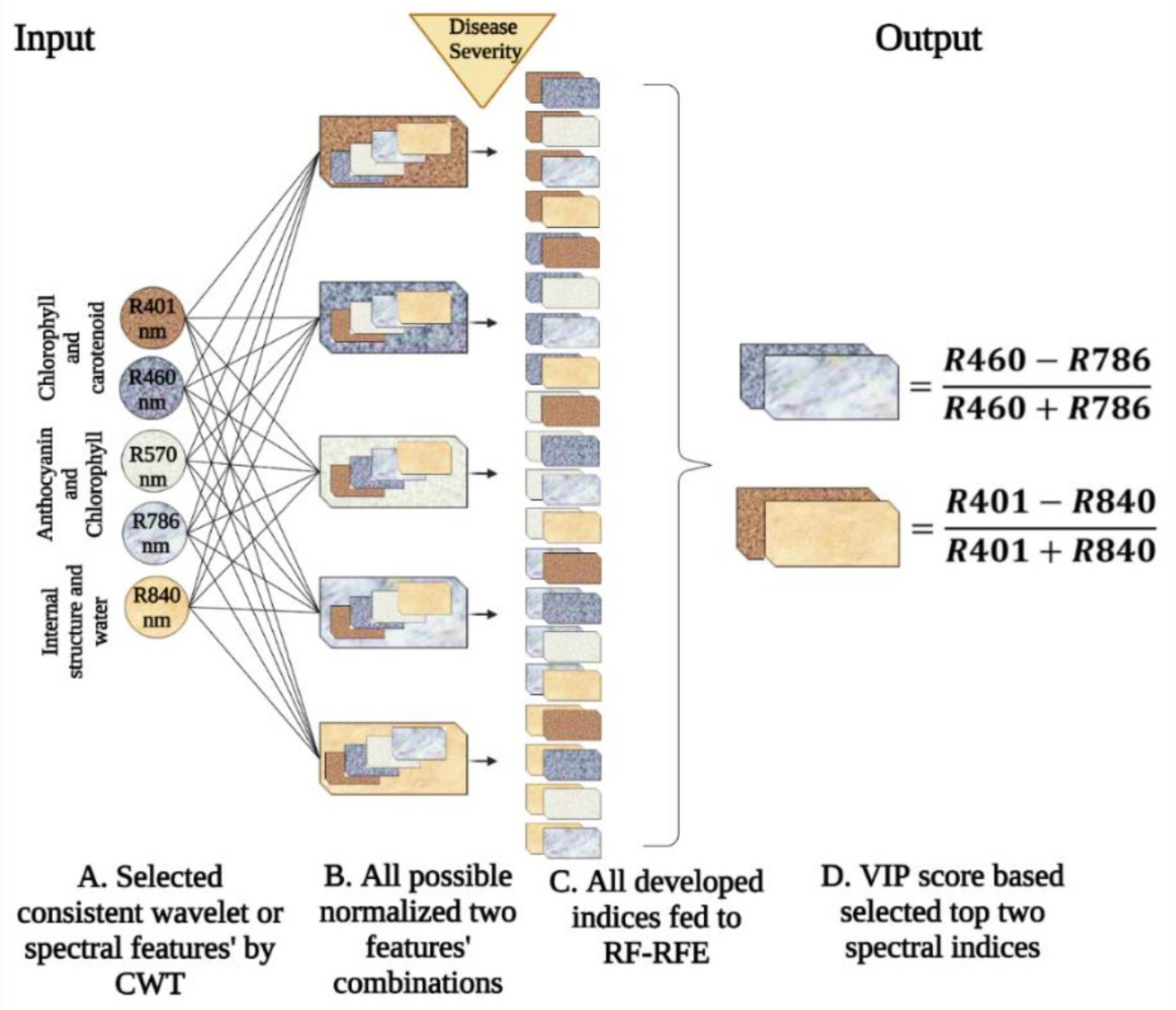
The selected five wavelengths after CWT analysis were subsequently employed to develop normalized difference indices. All possible normalized difference combinations were calculated and fed to RF-RFE for the selection of the disease spectral index of highest performance considering VIP (Figure 6). Resultantly, the best performing two wheat fusarium canopy indices—WFCI1 Equation (8) and WFCI2 Equation (9)—were selected, which make them comprehensive, conclusive, concisely described, transferable for future investigations and applicable in an independent manner.
Wheat   fusarium   canopy   index   WFCI 1 = R 401 R 840 R 401 + R 840 .
Wheat   fusarium   canopy   index   WFCI 2 = R 460 R 786 R 460 + R 786

3.4. Selection of Vegetation Indices at Canopy Scale

VIs are closely associated with physiological and biochemical plant parameters in both conditions (healthy and diseased). It is possible that they will be sensitive for disease detection and DS estimation because of their close relationship to the canopy’s physiological, biochemical and morphological parameters. The overall absolute R values (Table S1) for the year 2020 were higher than those for the next year, which was due to a higher disease incidence rate resulting in higher DS rates in the year 2020 than in 2021.
Considering the average correlation of individual VI for disease sensitivity (Table S1), we found NDVI (normalized difference vegetation index), mNDVI (Red-edge NDVI), PSNDa (pigment specific normalized difference), PSNDb (pigment specific normalized difference), PSNDc (pigment specific normalized difference), SIPI (structure-intensive pigment index), PSSRc (pigment specific simple ratio), PRIm4 (photochemical refl. index (670 and 570)), BRI2 (blue/red index), LIC1 (Lichtenthaler Index), NDWI (normalized difference water index), NDII (normalized difference water infrared index), and LIC2 (Lichtenthaler Index) are highly sensitive and negatively correlate with FHB disease. On the other hand, RI708′775, RGI (Red/green index), RR3 (Simple Ratio) and RR4 (Simple Ratio) have shown a positive correlation. Among highly sensitive VIs, NDVI; mNDVI; PSNDa; PSNDb; PSNDc; and SIPI belong to chlorophyll, PSSRc belongs to carotenoid and PRIm4 belongs to xanthophyll. These results show the degradation of the canopy pigments under FHB invasion. NDWI and NDII have also proved the water content damage under FHB invasion. On the other hand, VIs (RR3 and RR4) solidify the proof of stress increase in wheat canopy—in full agreement with their constituents for the plant stress category. Consequently, water-related VIs show high sensitivity after pigment-related VIs. After satisfactory results in the perspective of correlation analysis, we opted to select the top eight conventional VIs that have consistently performed better on average throughout both years of experiments and also made comparisons with newly developed indices (Table 1).

3.5. Separability Performance of Developed Indices against Conventional Spectral Indices

The performance of newly developed indices against conventional indices explains the proxy suitability standard for their optimality and validity for specific disease classification and estimation. The CA models for canopy were developed by using newly developed indices (Equations (8) and (9)) at canopy scales and highly sensitive conventional spectral indices by using canopy dataset and correlation-based selection of eight conventional spectral indices. Different machine learning classifiers (MLCs) were also employed to deeply explore the model development potential of developed indices.
WFCI1 (Table 2A) in 2020 manifested 83.33% CA at 5 DAI in RF and NN MLC; later on, at 8 DAI, CA increased to 100% in RF but NN maintained at 83.33% and fell behind SVM, which manifested 87.50% at the same dataset. While in 2021, Xgboost consistently lead over all MLC with 86.67 and 88.89% CA after 6 and 8 DAI, respectively. However, with SVM and RF, MLC showed 100% CA at 10 DAI while Xgboost maintained 88.89%. On the other hand, Knn MLC performed the worst for both years of experiments. WFCI2 (Table 2B) in 2020 produced 83.33% under RF MLC at 5 DAI and increased to 100% at 10 DAI, whereas SVM produced 100% CA at 8 DAI, but at 5 DAI, it showed less CA in comparison to RF. In 2021, SVM CA performance was better as it gave 73.33 and 100% CA at 6 and 8 DAI, respectively. Xgboost also performed better with CA of 73.33, 88.89 and 100% at 6, 8, and 10 DAI. For this index also, NN performance was weak but better than Knn. In 2020 (Table 2A,B), both of these newly developed indices manifested 100% CA for all MLC at 10 DAI with 18% DS. While in 2021, all MLC at 17 DAI showed full CA but RF, SVM and Xgboost produced 100% CA at 10 DAI with 19.34 DS.
Table 2C–E and Table S2A–E show the CA of conventional Vis, which in an overview have shown less CA. Conclusively, the newly developed indices have performed better than conventional Vis, whereas the average analysis has also been conducted in the next section.
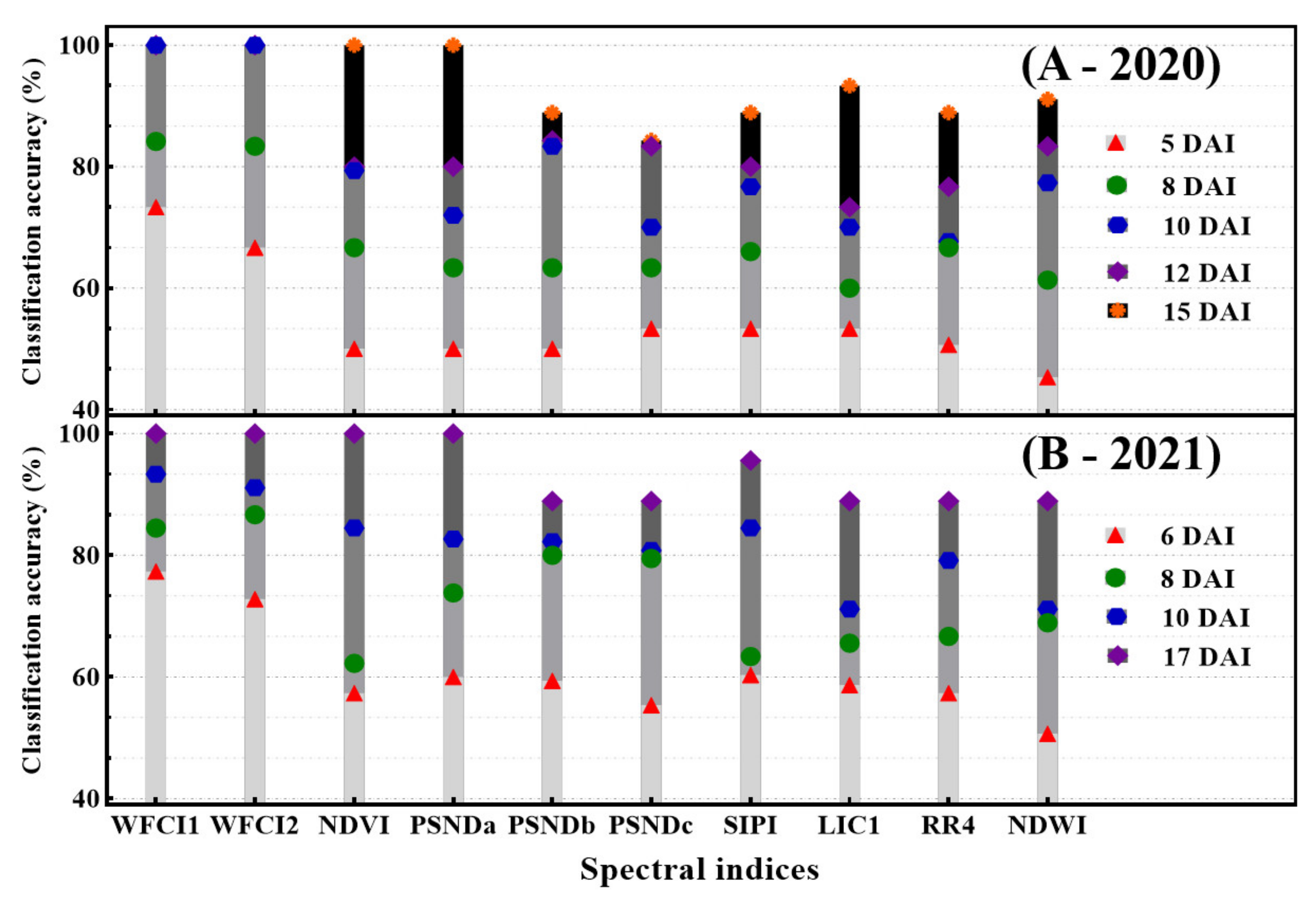
Figure 7 explains the calculated CA from all MLC in relevance to the number of DAI as an average classification accuracy (ACA) that shows the comparative performance of different VIs and developed indices for FHB detection at canopy scale. WFCI1 in 2020, produced 73.33% ACA at 5 DAI with 9.7% of DS, and at 8 DAI, it increased up to 84% and finally to 100% ACA at 10 DAI. Likewise, in 2021, ACA was observed at 77.3, 84.44, 93.33 and 100% at 6, 8, 10 and 17 DAI, respectively. Most specifically, it can be observed from Figure 7A,B that WFCI1 and WFCI2 have performed better and manifested high ACA compared to all other indices, which is due to the selection of most disease-relevant wavelengths. In particular, the ACA of canopy indices was higher for the early detection of the disease. More than 84% ACA was observed in 2020 and 2021 at 10.78 and 12.41% of DS, respectively.
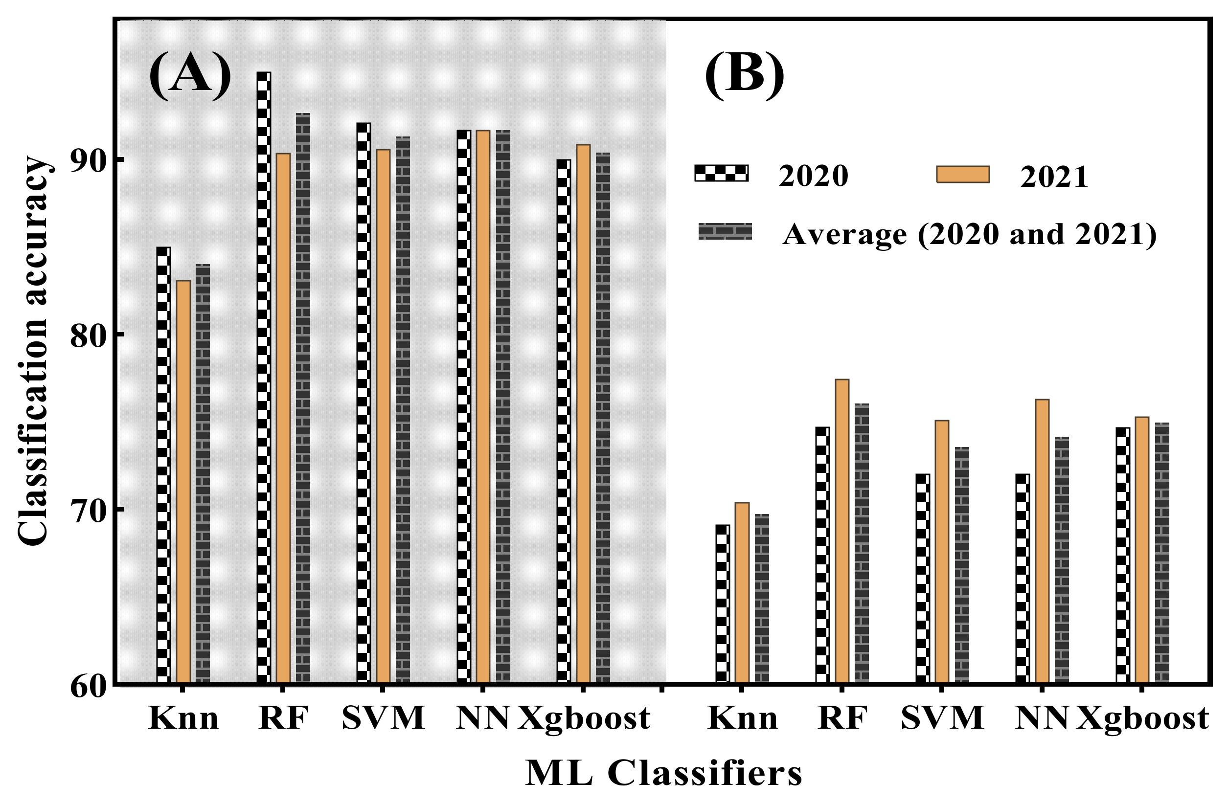
The CA performance of applied MLC was also evaluated by separately calculating the ACA of newly developed indices and conventional VIs. Similarly to previous CA findings, the ACA of developed and conventional VIs also does differed to a great extent. Figure 8A shows the ACA of MLC in 2020 and 2021 and an average of both years for canopy indices. On the behalf of 2020 ACA, MLC can be ranked in order as RF, SVM, NN, Xgboost and Knn with an ACA of 95, 92.08, 91.67, 90 and 85%, respectively. For 2021, MLC can be ranked as NN, Xgboost, SVM, RF and Knn with an ACA of 91.67, 90.83, 90.56, 90.33 and 83.09%, respectively. On the other hand, for average rankings, RF, NN, SVM, Xgboost and Knn had ACAs of 92.67, 91.67, 90.41 and 84.04%, respectively. Figure 8B demonstrates the ACA of MLC in 2020 and 2021 and an average of both years for conventional VIs. On the behalf of 2020 ACA, MLC can be ranked in order as RF, Xgboost, NN, SVM and Knn with an ACA of 74.72, 74.66, 72.03, 72.03 and 69.10%, respectively. For 2021, MLC ranked as RF, NN, Xgboost, SVM and Knn with ACAs of 77.43, 76.28, 75.28, 75.10 and 70.40%, respectively. On the other hand, for averages, MLC ranked as RF, Xgboost, NN, SVM and Knn had ACAs of 76.07, 74.97, 74.15, 73.56 and 69.75%, respectively. Conclusively, RF outperformed more outstandingly than the rest of the MLC, while Knn performed the worst in relevance to its competitors. Given the ACA, very comprehensive and validating results are generated that show the preciseness and suitability of canopy indices against conventional VIs. Moreover, the aptness, suitability and selection of MLC for disease classification in upcoming investigations were demonstrated.

3.6. Estimation of Disease Severity Using Conventional and Newly Developed Spectral Indices

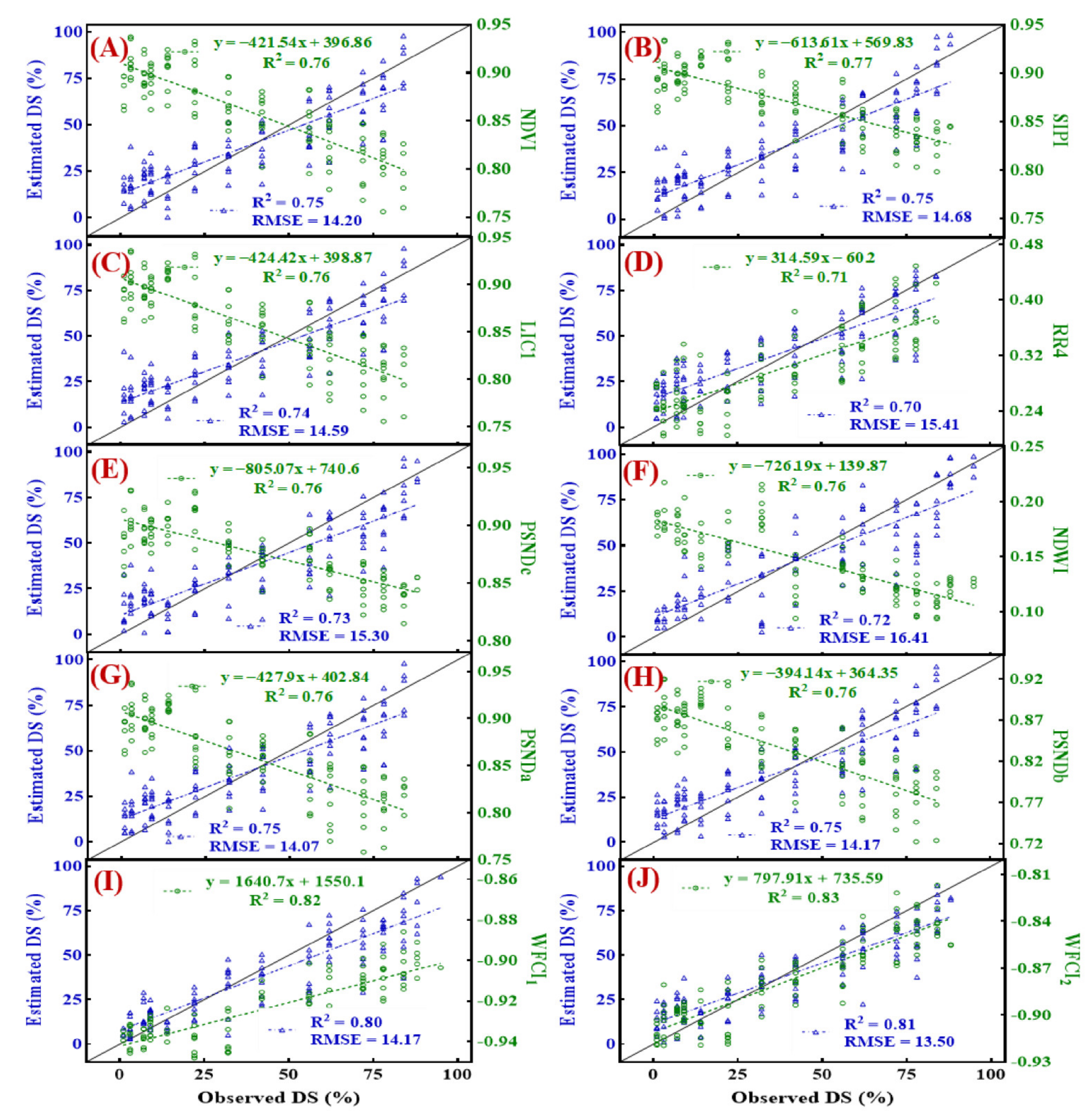
After observing the CA of all newly developed indices and VIs, we explored their potential for univariate disease estimation that provides the comparative evaluation of developed indices against conventional but highly sensitive VIs. For this, we employed the first year (2020) dataset to develop the quantitative relationship between index and DS and evaluated the performance of the developed univariate model through estimation of the DS employing the 2021 dataset. Resultantly, Figure 9 illustrates the quantitative relationship. In Figure 9A, NDVI constructed the model with R2 = 0.76 and estimated the DS with root mean square error (RMSE) of 14.20 and R2 = 0.75. Likewise, RR4 predicted the DS with an RMSE of 14.68 and R2 = 0.70 while the model was developed with an R2 of 0.71 (Figure 9D). The SIPI developed model with R2 of 0.77 manifested R2 = 0.75 with RMSE = 14.68 for its validation (Figure 9B). Likewise, LIC1 constructed a model with R2 = 0.76 and was validated with an exhibition of RMSE = 14.59 and R2 = 0.74 (Figure 9C). Figure 9E,F both constructed predictive models with R2 = 0.76 but for validation exhibited R2 = 0.73 with RMSE = 15.30 and R2 = 0.72 with an RMSE of 16.41, respectively. Likewise, Figure 9G,H built predictive models with R2 = 0.76 and for validation manifested similar R2 = 0.75 during its validation but with dissimilar RMSEs of 14.07 and 14.17, respectively. In general, all conventional VIs have shown reliability and stability for disease estimation in relevance to model construction coefficients of determination.
The canopy data-based developed indices WFCI1 and WFCI2 have also shown high predictive performance. WFCI1 constructed a model with R2 = 0.82 and validated its performance revealing RMSE = 14.17 and R2 = 0.80 (Figure 9I). Lastly, WFCI2 is the only index that manifested R2 = 0.83 during predictive model construction and also showed high R2 = 0.81 with RMSE = 13.50 (Figure 9J). Conclusively, a detailed examination of all the selected and developed indices concluded that newly developed indices have significantly better predictive abilities and estimation potential in relevance to conventional VIs when employing the same dataset and statistical approaches. Moreover, these can be practiced for the proxy determination of specific diseases.
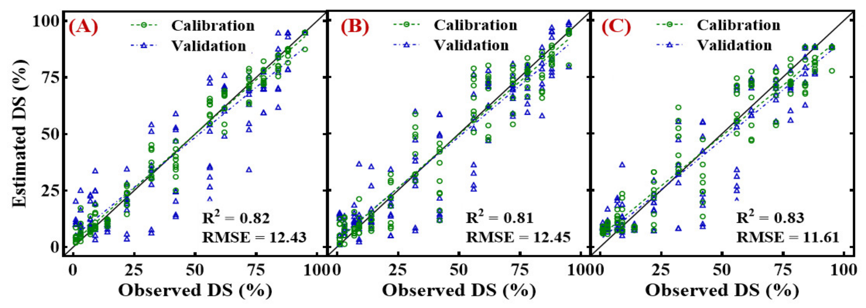
We further examined the potential of canopy-based newly developed indices in multivariate estimations using RFR, SVMR and KnnR by combining canopy-based indices (WFCI1 and WFCI2). Canopy-scale indices showed an estimation accuracy with an RMSE of 12.43 and R2 = 0.82 for RFR (Figure 10A), RMSE = 12.45 and R2 = 0.81 for SVMR (Figure 10B) and maximum in KnnR with an RMSE of 11.61 and R2 = 0.83 (Figure 10C). Conclusively, KnnR performed better and the results indicate that the developed indices have clearly shown their strength for disease estimation at canopy scale datasets. Thus, these results validate the specificity for FHB predictive abilities.

4. Discussion

4.1. Spectral and Photosynthetic Variations under Different Severities of FHB in the Wheat Canopy

The biophysical and spectral properties of the crop respond in a predictable manner under pathogen invasion, such as a reduction in water content, biomass, chlorophyll content and variations in corresponding optical reflectance, and this is true for all crops and pathogens studied [16,26]. As a result, understanding plant–pathogen interactions require the investigation of critical physiological mechanisms in the crop canopy in response to specific disease stresses. We measured canopy Pn, which showed a decreasing trend (Figure 4). Since Pn majorly relies on pigments (chlorophyll) and water contents. Thus, the decrease in Pn is also an indicator for pigment damage. Similar chlorophyll damage was also observed during fluorescence studies of wheat spikes [7,43].
The healthy and infected canopies had only slight reflectance differences in their appearance at early infection stages, and the red-edge region had only a slight reduction (Figure 11A). Early in the disease’s progression, the infected canopies began to show signs of FHB and the differences were more pronounced between healthy and infected plots in canopy reflectance. Supportively, Cao et al. [44] and Kobayashi et al. [45] had also found that spectral reflectance increased in the VIS and SWIR regions but decreased significantly in the NIR region. Infected canopies had higher spectral reflectance in green and red wavelengths than healthy ones (Figure 11B). Leaf pigments and green canopy fractions are primarily responsible for the red and green reflectances observed in these regions [46], and a similar reflectance trend was observed during spike damages due to FHB. Leaves with necrosis and chlorosis can have a negative impact on light transmission and reflectance in the green-and-red regions because they lack chlorophyll [47]; similarly, spikes also become deficient in chlorophyll contents. These findings suggest that FHB infestation reduces chlorophyll and photosynthetic activity in the infected canopies and alter reflectance in the visible range [47,48].
The SWIR (1300–2500 nm) at high DS showed typical vegetation stress properties in the FHB-induced canopy spectral reflectance, with reflectance in infected canopies rising in comparison to healthy ones (Figure 11C,D). According to Thenkabail and Lyon [10], leaf reflectance in the SWIR region is influenced by water absorption as well as carbohydrates and proteins, which suggests that FHB disease caused decreased water status, leading to low absorption and high reflectance in the SWIR region (Figure 11C,D). However, the spectral responses observed in the water and chlorophyll absorption regions of the wheat canopy may be similar to those caused by other stresses or diseases. Canopy reflectance can be used to identify specific stressors and diseases by recording canopy reflectance at multiple time points over an extended period. To date, the reflectance-based examination of FHB infected wheat canopy has not been practiced while a number of studies have examined the field wheat targeting the spikes only, employing diverse types of sensors [8,49].

4.2. Interpretation of Selected Spectral Bands and Vegetation Indices Development

The consistently selected five spectral bands at 401, 460, 570, 786 and 846 nm (Figure 5) are the FHB-specific wavebands used in this study. The selected wavelengths reveal that canopy damage is due to disruption in chlorophyll and carotenoid (401 and 460 nm), anthocyanin and chlorophyll (570 and 786 nm) and internal structure and water (840 nm). The authors of [50] designated the wavelengths 430 and 460 nm as chlorophyll a and chlorophyll b, respectively, and other studies asserted that chlorophyll decomposition and senescence occur in the ranges 400–530 nm and 550–740 nm, respectively [51]. Additionally, a decrease in chlorophyll content results in an increase in reflectance at 417 nm [6]. As a result, 401, 460 and 570 are excellent candidates for chlorophyll, while 570 characterizes the yellow range (550–650), which is indicative of several pigments, most notably anthocyanin and chlorophyll [52]. On the other hand, 786 nm in NIR explores the red-edge importance for disease detection. Meanwhile, 846 nm characterizes the structural variation in the near-infrared region of canopy reflectance. However, the role of water can also be speculated upon, as blighted spikes typically contain less water than healthy spikes [8,9,49,53]. The authors of [25] identified a similar waveband 866 nm for rice leaf blast. Wavelet studies have demonstrated its ability to detect features in the near-infrared [11,26]. Figure 5A–E demonstrate the VIS region’s dominance in disease response; however, wavelet analysis uncovered structural damage at 846 nm during the very early stages of disease proliferation.
Overall, conventional VIs (Table S3) related to chlorophyll, vegetation greenness and water-related indices consistently performed better. Additionally, other studies have shown that diseased leaves are prone to severe water deficits as a result of stomatal opening disorders [47]. Therefore, NDWI has also shown the potential as an FHB stress indicator. The negative correlations between DS and chlorophyll or greenness-related spectral indices such as LIC1, NDVI, PSNDa, PSNDb, PSNDc and SIPI, among others, are consistent with previous research demonstrating negative correlations between DS and NDVI and visible band spectral indices [20,54]. A strong correlation between VIs and DS suggests that, at canopy scales, HR can capture canopy DS and biophysical variations in diseased leaves [55,56]. Numerous studies have developed spectral indices by combining two or more relevant wavelengths from the VIS, NIR or SWIR reflectance regions specific to a disease or other objective problems [19,25]. Accordingly, our study has also developed FHB canopy disease-specific indices ((WFCI1 Equation (8) and WFCI2 Equation (9)) employing selected wavebands. The results (Table 2) of developed indices have also proved their relevance, suitability, optimality, functionality, classification and estimation potential. Regional-level studies can also be considered for the further validation of selected and developed indices.
The newly developed indices have performed better for CA at a canopy scale. Subsequently, the models for disease estimation are developed by employing all newly developed indices and also compared with conventional indices. The single variable and multiple variables are used for univariate and multivariate disease estimation approaches [57]. The comparative performance of disease specific or newly developed indices for model fitting is highly improved against conventional VIs (Figure 9), which is likely due to previous studies [18]. In addition, the results have concluded that multivariate modeling manifest better disease determination accuracy in comparison to univariate models [18]. Likewise, in our study, multivariate models obtained better estimation accuracy during the combination of both indices (Figure 10A–C). In multivariate analysis, WFCI1-WFCI2-KnnR (R2 = 0.86, RMSE = 10.36) revealed the best results for canopy scale disease estimation. Based on these results, a precise FHB monitoring program can be developed. Moreover, the better disease estimation performance of models through disease specific indices have also been proved by previous findings [58,59].

4.3. Disease Classification with Different Machine Learning Classifiers

The most up-to-date strategy involves combining spectral wavelengths that are relevant to objective problems such as disease, nutrients, cultivar type and many others. However, the developed combination is needed to be examined under diverse approaches to fully validate its modeling performance. Therefore, a comparative analysis is necessary to ensure the robustness and transferability of developed indices through the accessibility of numerous ML techniques that have different constituents for feature selection and classification. Several scientists used different MLCs to categorize diseases [16,25]. Due to subtle changes in reflectance, visual and conventional spectral analysis for pre-symptomatic disease detection is difficult [11,19]. Various MLC approaches have been used to classify diseases in numerous studies [11,16,25,49,59]. There are different datasets used in this study, each with its own number of samples that could pose a challenge to CA, including the datasets of WFCI1 and WFCI2. The CA results (Table 2), which showed a varied response for MLC and demonstrated the relevance to FHB, backed up this claim. SVM, Knn, RF and NN predictive models have been used in similar studies to classify plants [16,25]. However, as far as we know, the Xgboost algorithm has not been tested for disease classification in plants to date. In contrast, it manifested a CA of 84.80% without engaging FS and 85.60% through FS for neurotic diseases [60]. Similarly, it was 99.75% accurate in diagnosing kidney disease. In addition to these advantages, it runs data more quickly and consumes less memory than other machine learning algorithms [61]. As a result of this efficiency, our study has greatly benefited from a reduction in computational time and a significant increase in speed. Knn was the only MLC to show low CA compared to others.

4.4. Potential Constraints for Application Possibilities

To the best of our knowledge, there has been no precise monitoring of wheat canopy with FHB interaction for the net photosynthesis (Figure 4) of spikes. This could be a compelling indicator for disease studies and to see the fingerprints of FHB invasion on spike photosynthesis. After that, large-scale FHB invasion detection inspections are possible. Numerous studies have used spectral indices at spike-scale to investigate disease detection, likewise, NDVI, PRI, PSSRa, PSSRb, PSSRc and WI were investigated for FHB analysis [9]. Other studies have shown that spectral indices in the VIS and NIR regions can be used to identify FHB [6,7,62]. The WFCI1 and WFCI2 have confirmed and demonstrated their potential for FHB disease classifications at different DAI. Automated high-throughput phenotyping systems that can detect disease in real-time and with high accuracy could use the newly developed methodology specific to canopy scales. UAV applications can also validate its performance.
FHB detection methods and disease-specific indices developed for the classification and estimation purposes have been found to be effective. However, known issues, such as environmental factors, fungal growth and crop symmetry, may be limiting factors. Ashourloo et al. [63] found that different pathogen quantities at the same DS could affect reflectance and that the CA of sensitive features could suffer as a result. Due to their spectral nature, all selected features have a lower dimensionality and collinearity. Because of this, it is possible to create an instrument with fewer spectral data points that could be more useful. Our study confirms that investigation using these indices could be an innovative approach to monitor canopy scale disease, which could save time and money.

5. Conclusions

The purpose of this study was to investigate the spectral characteristics of wheat canopy’s FHB, to detect it as early as possible at the canopy scale and to accurately monitor DS. Following inoculation, the results showed that Pn decreased significantly with increasing DS. It was found that the spectral reflectance of infected canopies increased in the visible range and decreased significantly in the near-infrared range. After the selection of sensitive bands and development of normalized indices, we also calculated 92 VIs that were related to different biophysical parameters to observe if they were indicators of disease stress and to compare against newly developed indices. The detailed conclusions can be drawn as follows:
  • The conventional VIs (NDVI, PSNDa, PSNDb, PSNDc, LIC1, SIPI, RR4 and NDWI) were found to be highly correlated with DS (Table 1). The VIs associated with plant water and chlorophyll status were found to be negatively correlated with canopy DS. Using machine learning classifiers (MLC), including an RF model based on each consistently selected VIs, WFCI1 and WFCI2 consistently outperformed the other four MLCs (Knn, SVM, NN and Xgboost) in terms of distinguishing between healthy and infected canopies over the course of two years. RF manifested 83.33% CA at DS of 9.73% and improved to 100% CA at a DS of 10.78% at 8 DAI in the year 2020.
  • The linear regression models based on WFCI1 and WFCI2 with independent data produced R2 values of 0.80, and 0.81, respectively, had root mean square errors (RMSEs) of 14.17 and 13.50, respectively. In multivariate models, the models WFCI1-WFCI2-KnnR (R2 = 0.83, RMSE = 11.61) revealed the best results for canopy scale disease estimation.
The hyperspectral canopy measurements in combination with the MLC were able to distinguish wheat FHB-diseased canopies from healthy canopies with high accuracy. Research that leads toward a better understanding of the interactions between disease progression, canopy structure and physiological variations will improve the ability to measure and identify plant diseases using remote sensing technologies in the near future.

Supplementary Materials

The following supporting information can be downloaded at: https://www.mdpi.com/article/10.3390/rs14122784/s1, Table S1: Correlation coefficients (R) through Pearson Correlation Analysis between vegetation indices (categorized and enlisted in article) and wheat fusarium head blight disease severity (p < 0.05); Table S2: Classification accuracy of the conventional spectral indices employing different machine learning classifiers.; Table S3: Vegetation indices calculated for this study and their detailed information. References [6,16,19,20,51,56,64,65,66,67,68,69,70,71,72,73,74,75,76,77,78,79,80,81,82,83,84,85,86,87,88,89,90,91,92,93,94,95] are cited in the Supplementary Materials.

Author Contributions

Conceptualization, Y.Z. and X.Y.; methodology, H.Z., G.M. and I.H.K.; software, L.T. and G.M.; validation, X.Y., T.C. and W.C.; formal analysis, G.M.; investigation, G.M. and H.Z.; resources, W.C., Y.Z., H.J. and G.L.; writing—original draft preparation, X.Y., H.Z., T.C. and I.H.K.; writing—review and editing, X.Y., T.C., Y.Z. and W.C.; supervision, Y.Z., X.Y., T.C., Y.T. and G.L.; project administration, X.Y.; funding acquisition, X.Y. and Y.Z. All authors have read and agreed to the published version of the manuscript.

Funding

We thank the National Key Research and Development Program of China (2019YFE0125500-04), National Natural Science Foundation of China (31671582), the Advanced Research Project of Civil Aerospace Technologies (D040104), the Key Projects (Advanced Technology) of Jiangsu Province (BE 2019383) and Jiangsu Collaborative Innovation Center for Modern Crop Production (JCICMCP) for funding.

Data Availability Statement

Not applicable.

Conflicts of Interest

The authors declare no conflict of interest. The funders had no role in the design of the study; in the collection, analyses, or interpretation of data; in the writing of the manuscript; or in the decision to publish the results.

Abbreviations

AcronymsExtended Meaning
ACAAverage classification accuracy
CSBsConsistent spectral bands
CWTContinuous wavelet transform
DAIDays after inoculation
DWTDiscrete wavelet transform
FHBFusarium head blight
HRHyperspectral reflectance
HSIHyperspectral imaging
KnnK nearest neighbor
KnnRK nearest neighbor regression
MLMachine learning
MLCMachine learning classifiers
NNNeural net
PnPhotosynthesis rate
R2Coefficient of determination
RFRandom forest
RFRRandom forest regression
RF-RFERandom forest—recursive feature elimination
RMSERoot mean square error
SCCSpike chlorophyll contents
SVMSupport vector machine
SVMRSupport vector machine regression
VIPVariable importance score
XgboostExtreme gradient boost

References

  1. Goswami, R.S.; Kistler, H.C. Heading for disaster: Fusarium graminearum on cereal crops. Mol. Plant Pathol. 2004, 5, 515–525. [Google Scholar] [CrossRef] [PubMed]
  2. McBeath, J.H.; McBeath, J. Plant diseases, pests and food security. In Environmental Change and Food Security in China; Springer: Berlin/Heidelberg, Germany, 2010; pp. 117–156. [Google Scholar]
  3. Li, W.G.; Chen, H.; Jin, Z.T.; Zhang, Z.Z.; Ge, G.X.; Ji, F.J. Remote sensing monitoring of winter wheat scab based on suitable scale selection. J. Triticeae Crops 2018, 38, 1374–1380. [Google Scholar]
  4. Khan, I.H.; Liu, H.; Li, W.; Cao, A.; Wang, X.; Liu, H.; Cheng, T.; Tian, Y.; Zhu, Y.; Cao, W. Early Detection of Powdery Mildew Disease and Accurate Quantification of Its Severity Using Hyperspectral Images in Wheat. Remote Sens. 2021, 13, 3612. [Google Scholar] [CrossRef]
  5. Li, X.; Zhang, Y.; Bao, Y.; Luo, J.; Jin, X.; Xu, X.; Song, X.; Yang, G. Exploring the best hyperspectral features for LAI estimation using partial least squares regression. Remote Sens. 2014, 6, 6221–6241. [Google Scholar] [CrossRef] [Green Version]
  6. Zhang, N.; Pan, Y.; Feng, H.; Zhao, X.; Yang, X.; Ding, C.; Yang, G. Development of Fusarium head blight classification index using hyperspectral microscopy images of winter wheat spikelets. Biosyst. Eng. 2019, 186, 83–99. [Google Scholar] [CrossRef]
  7. Bauriegel, E.; Giebel, A.; Geyer, M.; Schmidt, U.; Herppich, W.B. Early detection of Fusarium infection in wheat using hyper-spectral imaging. Comput. Electron. Agric. 2011, 75, 304–312. [Google Scholar] [CrossRef]
  8. Jin, X.; Jie, L.; Wang, S.; Qi, H.J.; Li, S.W. Classifying wheat hyperspectral pixels of healthy heads and Fusarium head blight disease using a deep neural network in the wild field. Remote Sens. 2018, 10, 395. [Google Scholar] [CrossRef] [Green Version]
  9. Mahlein, A.-K.; Alisaac, E.; Al Masri, A.; Behmann, J.; Dehne, H.-W.; Oerke, E.-C. Comparison and combination of thermal, fluorescence, and hyperspectral imaging for monitoring fusarium head blight of wheat on spikelet scale. Sensors 2019, 19, 2281. [Google Scholar] [CrossRef] [Green Version]
  10. Thenkabail, P.S.; Lyon, J.G. Hyperspectral Remote Sensing of Vegetation; CRC Press: Boca Raton, FL, USA, 2016. [Google Scholar]
  11. Ma, H.; Huang, W.; Jing, Y.; Pignatti, S.; Laneve, G.; Dong, Y.; Ye, H.; Liu, L.; Guo, A.; Jiang, J. Identification of Fusarium head blight in winter wheat ears using continuous wavelet analysis. Sensors 2020, 20, 20. [Google Scholar] [CrossRef] [Green Version]
  12. Huang, L.; Wu, Z.; Huang, W.; Ma, H.; Zhao, J. Identification of fusarium head blight in winter wheat ears based on fisher’s linear discriminant analysis and a support vector machine. Appl. Sci. 2019, 9, 3894. [Google Scholar] [CrossRef] [Green Version]
  13. Zheng, H.; Cheng, T.; Zhou, M.; Li, D.; Yao, X.; Tian, Y.; Cao, W.; Zhu, Y. Improved estimation of rice aboveground biomass combining textural and spectral analysis of UAV imagery. Precis. Agric. 2019, 20, 611–629. [Google Scholar] [CrossRef]
  14. Yu, K.; Anderegg, J.; Mikaberidze, A.; Karisto, P.; Mascher, F.; McDonald, B.A.; Walter, A.; Hund, A. Hyperspectral canopy sensing of wheat septoria tritici blotch disease. Front. Plant Sci. 2018, 9, 1195. [Google Scholar] [CrossRef] [PubMed] [Green Version]
  15. Delalieux, S.; Somers, B.; Verstraeten, W.W.; Van Aardt, J.A.N.; Keulemans, W.; Coppin, P. Hyperspectral indices to diagnose leaf biotic stress of apple plants, considering leaf phenology. Int. J. Remote Sens. 2009, 30, 1887–1912. [Google Scholar] [CrossRef]
  16. Zarco-Tejada, P.J.; Camino, C.; Beck, P.S.A.; Calderon, R.; Hornero, A.; Hernández-Clemente, R.; Kattenborn, T.; Montes-Borrego, M.; Susca, L.; Morelli, M. Previsual symptoms of Xylella fastidiosa infection revealed in spectral plant-trait alterations. Nat. Plants 2018, 4, 432–439. [Google Scholar] [CrossRef] [PubMed]
  17. Zarco-Tejada, P.J.; Miller, J.R.; Noland, T.L.; Mohammed, G.H.; Sampson, P.H. Scaling-up and model inversion methods with narrowband optical indices for chlorophyll content estimation in closed forest canopies with hyperspectral data. IEEE Trans. Geosci. Remote Sens. 2001, 39, 1491–1507. [Google Scholar] [CrossRef] [Green Version]
  18. Zhang, J.; Pu, R.; Loraamm, R.W.; Yang, G.; Wang, J. Comparison between wavelet spectral features and conventional spectral features in detecting yellow rust for winter wheat. Comput. Electron. Agric. 2014, 100, 79–87. [Google Scholar] [CrossRef]
  19. Mahlein, A.K.; Rumpf, T.; Welke, P.; Dehne, H.W.; Plümer, L.; Steiner, U.; Oerke, E.C. Development of spectral indices for detecting and identifying plant diseases. Remote Sens. Environ. 2013, 128, 21–30. [Google Scholar] [CrossRef]
  20. Ashourloo, D.; Mobasheri, M.R.; Huete, A. Developing two spectral disease indices for detection of wheat leaf rust (Pucciniatriticina). Remote Sens. 2014, 6, 4723–4740. [Google Scholar] [CrossRef] [Green Version]
  21. Luedeling, E.; Hale, A.; Zhang, M.; Bentley, W.J.; Dharmasri, L.C. Remote sensing of spider mite damage in California peach orchards. Int. J. Appl. Earth Obs. Geoinf. 2009, 11, 244–255. [Google Scholar] [CrossRef]
  22. Liu, X.-n.; Liu, H.-k.; Huang, Y.-f.; Ye, Y.-l. Relationships between nitrogen application rate soil nitrate-nitrogen plant nitrogen concentration and wheat scab. J. Plant Nutr. Fertil. 2015, 21, 306–317. [Google Scholar]
  23. Chang, T.-G.; Song, Q.-F.; Zhao, H.-L.; Chang, S.; Xin, C.; Qu, M.; Zhu, X.-G. An in situ approach to characterizing photosynthetic gas exchange of rice panicle. Plant Methods 2020, 16, 1–14. [Google Scholar] [CrossRef] [PubMed]
  24. Bellman, R.E. Perturbation Techniques in Mathematics, Engineering and Physics; Courier Corporation: North Chelmsford, MA, USA, 2003. [Google Scholar]
  25. Tian, L.; Xue, B.; Wang, Z.; Li, D.; Yao, X.; Cao, Q.; Zhu, Y.; Cao, W.; Cheng, T. Spectroscopic detection of rice leaf blast infection from asymptomatic to mild stages with integrated machine learning and feature selection. Remote Sens. Environ. 2021, 257, 112350. [Google Scholar] [CrossRef]
  26. Cheng, T.; Rivard, B.; Sánchez-Azofeifa, G.A.; Feng, J.; Calvo-Polanco, M. Continuous wavelet analysis for the detection of green attack damage due to mountain pine beetle infestation. Remote Sens. Environ. 2010, 114, 899–910. [Google Scholar] [CrossRef]
  27. Blackburn, G.A.; Ferwerda, J.G. Retrieval of chlorophyll concentration from leaf reflectance spectra using wavelet analysis. Remote Sens. Environ. 2008, 112, 1614–1632. [Google Scholar] [CrossRef]
  28. Bruce, L.M.; Li, J. Wavelets for computationally efficient hyperspectral derivative analysis. IEEE Trans. Geosci. Remote Sens. 2001, 39, 1540–1546. [Google Scholar] [CrossRef] [Green Version]
  29. Rivard, B.; Feng, J.; Gallie, A.; Sanchez-Azofeifa, A. Continuous wavelets for the improved use of spectral libraries and hyperspectral data. Remote Sens. Environ. 2008, 112, 2850–2862. [Google Scholar] [CrossRef]
  30. Gregorutti, B.; Michel, B.; Saint-Pierre, P. Grouped variable importance with random forests and application to multiple functional data analysis. Comput. Stat. Data Anal. 2015, 90, 15–35. [Google Scholar] [CrossRef] [Green Version]
  31. Lorena, A.C.; Jacintho, L.F.O.; Siqueira, M.F.; De Giovanni, R.; Lohmann, L.G.; De Carvalho, A.C.; Yamamoto, M. Comparing machine learning classifiers in potential distribution modelling. Expert Syst. Appl. 2011, 38, 5268–5275. [Google Scholar] [CrossRef]
  32. Gorunescu, F. Data Mining: Concepts, Models and Techniques; Springer Science & Business Media: Berlin/Heidelberg, Germany, 2011; Volume 12. [Google Scholar]
  33. Ayyash, M. A framework for a Minkowski distance based multi metric quality of service monitoring infrastructure for mobile ad hoc networks. Int. J. Electr. Eng. Inform. 2012, 4, 289. [Google Scholar] [CrossRef]
  34. Chang, C.-C.; Lin, C.-J. Training v-support vector classifiers: Theory and algorithms. Neural Comput. 2001, 13, 2119–2147. [Google Scholar] [CrossRef]
  35. Belgiu, M.; Drăguţ, L. Random forest in remote sensing: A review of applications and future directions. ISPRS J. Photogramm. Remote Sens. 2016, 114, 24–31. [Google Scholar] [CrossRef]
  36. Gurney, K. An Introduction to Neural Networks; CRC Press: Boca Raton, FL, USA, 2018. [Google Scholar]
  37. Chen, T.; Guestrin, C. Xgboost: A scalable tree boosting system. In Proceedings of the KDD ’16: Proceedings of the 22nd ACM SIGKDD International Conference on Knowledge Discovery and Data Mining, San Francisco, CA, USA, 13–17 August 2016; Association for Computing Machinery: New York, NY, USA, 2016; pp. 785–794. [Google Scholar]
  38. Schliep, K.; Hechenbichler, K.; Lizee, A. kknn: Weighted k-Nearest Neighbors, version 1.3.1; R Foundation for Statistical Computing: Vienna, Austria, 2016; Available online: https://cran.r-project.org/web/packages/kknn/kknn.pdf (accessed on 3 April 2022).
  39. RcolorBrewer, S.; Liaw, M.A. Package ‘randomForest’, version 4.6-14; University of California: Berkeley, CA, USA, 2018. [Google Scholar]
  40. Meyer, D.; Dimitriadou, E.; Hornik, K.; Weingessel, A.; Leisch, F. e1071: Misc Functions of the Department of Statistics, Probability Theory Group (Formerly: E1071), R package version 1.7-2; Vienna University of Technology: Vienna, Austria, 2020. [Google Scholar]
  41. Fritsch, S.; Guenther, F.; Guenther, M.F. Training of Neural Networks—Package ‘neuralnet’, version 1.44.2; R Foundation for Statistical Computing: Vienna, Austria, 2019; Available online: https://cran.r-project.org/web/packages/neuralnet/neuralnet (accessed on 7 February 2022).
  42. Chen, T.; He, T.; Benesty, M.; Khotilovich, V. Extreme Gradient Boosting–Package ‘xgboost’; R Version 1.6.0.1; R Foundation for Statistical Computing: Vienna, Austria, 2019; Available online: https://cran.r-project.org/web/packages/xgboost/vignettes/xgboost (accessed on 25 June 2021).
  43. Bauriegel, E.; Brabandt, H.; Gärber, U.; Herppich, W.B. Chlorophyll fluorescence imaging to facilitate breeding of Bremia lactucae-resistant lettuce cultivars. Comput. Electron. Agric. 2014, 105, 74–82. [Google Scholar] [CrossRef]
  44. Cao, X.; Luo, Y.; Zhou, Y.; Duan, X.; Cheng, D. Detection of powdery mildew in two winter wheat cultivars using canopy hyperspectral reflectance. Crop Prot. 2013, 45, 124–131. [Google Scholar] [CrossRef]
  45. Kobayashi, T.; Kanda, E.; Kitada, K.; Ishiguro, K.; Torigoe, Y. Detection of rice panicle blast with multispectral radiometer and the potential of using airborne multispectral scanners. Phytopathology 2001, 91, 316–323. [Google Scholar] [CrossRef] [PubMed] [Green Version]
  46. Ustin, S.L.; Gitelson, A.A.; Jacquemoud, S.; Schaepman, M.; Asner, G.P.; Gamon, J.A.; Zarco-Tejada, P. Retrieval of foliar information about plant pigment systems from high resolution spectroscopy. Remote Sens. Environ. 2009, 113, S67–S77. [Google Scholar] [CrossRef] [Green Version]
  47. Oerke, E.-C.; Herzog, K.; Toepfer, R. Hyperspectral phenotyping of the reaction of grapevine genotypes to Plasmopara viticola. J. Exp. Bot. 2016, 67, 5529–5543. [Google Scholar] [CrossRef] [Green Version]
  48. Mahlein, A.-K. Plant disease detection by imaging sensors–parallels and specific demands for precision agriculture and plant phenotyping. Plant Dis. 2016, 100, 241–251. [Google Scholar] [CrossRef] [Green Version]
  49. Huang, L.; Zhang, H.; Huang, W.; Dong, Y.; Ye, H.; Ma, H.; Zhao, J. Identification of Fusarium head blight in wheat ears using vertical angle-based reflectance spectroscopy. Arab. J. Geosci. 2021, 14, 423. [Google Scholar] [CrossRef]
  50. Jensen, J.R. Remote Sensing of the Environment–An Earth Resource Perspective; Reprint edition; Pearson Education: Noida, India, 2002. [Google Scholar]
  51. Merzlyak, M.N.; Gitelson, A.A.; Chivkunova, O.B.; Rakitin, V.Y. Non-destructive optical detection of pigment changes during leaf senescence and fruit ripening. Physiol. Plant. 1999, 106, 135–141. [Google Scholar] [CrossRef] [Green Version]
  52. Féret, J.B.; Gitelson, A.A.; Noble, S.D.; Jacquemoud, S. PROSPECT-D: Towards modeling leaf optical properties through a complete lifecycle. Remote Sens. Environ. 2017, 193, 204–215. [Google Scholar] [CrossRef] [Green Version]
  53. Al Masri, A.; Hau, B.; Dehne, H.W.; Mahlein, A.K.; Oerke, E.C. Impact of primary infection site of Fusarium species on head blight development in wheat ears evaluated by IR-thermography. Eur. J. Plant Pathol. 2017, 147, 855–868. [Google Scholar] [CrossRef]
  54. Steddom, K.; Bredehoeft, M.W.; Khan, M.; Rush, C.M. Comparison of visual and multispectral radiometric disease evaluations of Cercospora leaf spot of sugar beet. Plant Dis. 2005, 89, 153–158. [Google Scholar] [CrossRef] [PubMed] [Green Version]
  55. Bajwa, S.G.; Rupe, J.C.; Mason, J. Soybean disease monitoring with leaf reflectance. Remote Sens. 2017, 9, 127. [Google Scholar] [CrossRef] [Green Version]
  56. Penuelas, J.; Baret, F.; Filella, I. Semi-empirical indices to assess carotenoids/chlorophyll a ratio from leaf spectral reflectance. Photosynthetica 1995, 31, 221–230. [Google Scholar]
  57. Feng, Z.-H.; Wang, L.-Y.; Yang, Z.-Q.; Zhang, Y.-Y.; Li, X.; Song, L.; He, L.; Duan, J.-Z.; Feng, W. Hyperspectral Monitoring of Powdery Mildew Disease Severity in Wheat Based on Machine Learning. Front. Plant Sci. 2022, 13, 828454. [Google Scholar] [CrossRef]
  58. Guo, W.; Yang, Y.; Zhao, H.; Song, R.; Dong, P.; Jin, Q.; Baig, M.H.A.; Liu, Z.; Yang, Z. Winter Wheat Take-All Disease Index Estimation Model Based on Hyperspectral Data. Appl. Sci. 2021, 11, 9230. [Google Scholar] [CrossRef]
  59. Huang, L.; Zhang, H.; Ding, W.; Huang, W.; Hu, T.; Zhao, J. Monitoring of wheat scab using the specific spectral index from ASD hyperspectral dataset. J. Spectrosc. 2019, 2019, 9153195. [Google Scholar] [CrossRef]
  60. Abdurrahman, G.; Sintawati, M. Implementation of xgboost for classification of parkinson’s disease. J. Phys. Conf. Ser. 2020, 1538, 012024. [Google Scholar] [CrossRef]
  61. Aydin, Z.E.; Ozturk, Z.K. XGBoost feature selection on Chronic kidney disease diagnosis. In Proceedings of the IV International Conference on Data Science and Applications (ICONDATA’20), Eskisehir, Turkey, 4–6 June 2021. [Google Scholar]
  62. Alisaac, E.; Behmann, J.; Kuska, M.T.; Dehne, H.W.; Mahlein, A.K. Hyperspectral quantification of wheat resistance to Fusarium head blight: Comparison of two Fusarium species. Eur. J. Plant Pathol. 2018, 152, 869–884. [Google Scholar] [CrossRef]
  63. Ashourloo, D.; Aghighi, H.; Matkan, A.A.; Mobasheri, M.R.; Rad, A.M. An investigation into machine learning regression techniques for the leaf rust disease detection using hyperspectral measurement. IEEE J. Sel. Top. Appl. Earth Obs. Remote Sens. 2016, 9, 4344–4351. [Google Scholar] [CrossRef]
  64. Huang, W.; Guan, Q.; Luo, J.; Zhang, J.; Zhao, J.; Liang, D.; Huang, L.; Zhang, D. New optimized spectral indices for identifying and monitoring winter wheat diseases. IEEE J. Sel. Top. Appl. Earth Obs. Remote Sens. 2014, 7, 2516–2524. [Google Scholar] [CrossRef]
  65. Gitelson, A.A.; Buschmann, C.; Lichtenthaler, H.K. The chlorophyll fluorescence ratio F735/F700 as an accurate measure of the chlorophyll content in plants. Remote Sens. Environ. 1999, 69, 296–302. [Google Scholar] [CrossRef]
  66. Sims, D.A.; Gamon, J.A. Relationships between leaf pigment content and spectral reflectance across a wide range of species, leaf structures and developmental stages. Remote Sens. Environ. 2002, 81, 337–354. [Google Scholar] [CrossRef]
  67. Blackburn, G.A. Spectral indices for estimating photosynthetic pigment concentrations: A test using senescent tree leaves. Int. J. Remote Sens. 1998, 19, 657–675. [Google Scholar] [CrossRef]
  68. Blackburn, G.A. Relationships between spectral reflectance and pigment concentrations in stacks of deciduous broadleaves. Remote Sens. Environ. 1999, 70, 224–237. [Google Scholar] [CrossRef]
  69. Chappelle, E.W.; Kim, M.S.; McMurtrey Iii, J.E. Ratio analysis of reflectance spectra (RARS): An algorithm for the remote estimation of the concentrations of chlorophyll a, chlorophyll b, and carotenoids in soybean leaves. Remote Sens. Environ. 1992, 39, 239–247. [Google Scholar] [CrossRef]
  70. Rouse, J.W.; Haas, R.H.; Schell, J.A.; Deering, D.W.; Harlan, J.C. Monitoring the vernal advancement and retrogradation (green wave effect) of natural vegetation. In NASA/GSFC Type III Final Report; NASA: Greenbelt, MD, USA, 1974. [Google Scholar]
  71. Gitelson, A.; Merzlyak, M.N. Quantitative estimation of chlorophyll-a using reflectance spectra: Experiments with autumn chestnut and maple leaves. J. Photochem. Photobiol. B Biol. 1994, 22, 247–252. [Google Scholar] [CrossRef]
  72. Blackburn, G.A. Quantifying chlorophylls and caroteniods at leaf and canopy scales: An evaluation of some hyperspectral approaches. Remote Sens. Environ. 1998, 66, 273–285. [Google Scholar] [CrossRef]
  73. Maccioni, A.; Agati, G.; Mazzinghi, P. New vegetation indices for remote measurement of chlorophylls based on leaf directional reflectance spectra. J. Photochem. Photobiol. B Biol. 2001, 61, 52–61. [Google Scholar] [CrossRef]
  74. Dash, J.; Curran, P.J. The MERIS Terrestrial Chlorophyll Index; Taylor & Francis: Abingdon, UK, 2004. [Google Scholar]
  75. Datt, B. Remote sensing of chlorophyll a, chlorophyll b, chlorophyll a + b, and total carotenoid content in eucalyptus leaves. Remote Sens. Environ. 1998, 66, 111–121. [Google Scholar] [CrossRef]
  76. Datt, B. A new reflectance index for remote sensing of chlorophyll content in higher plants: Tests using Eucalyptus leaves. J. Plant Physiol. 1999, 154, 30–36. [Google Scholar] [CrossRef]
  77. Vogelmann, J.E.; Rock, B.N.; Moss, D.M. Red edge spectral measurements from sugar maple leaves. Int. J. Remote Sens. 1993, 14, 1563–1575. [Google Scholar] [CrossRef]
  78. Gitelson, A.A.; Merzlyak, M.N. Signature analysis of leaf reflectance spectra: Algorithm development for remote sensing of chlorophyll. J. Plant Physiol. 1996, 148, 494–500. [Google Scholar] [CrossRef]
  79. Haboudane, D.; Miller, J.R.; Tremblay, N.; Zarco-Tejada, P.J.; Dextraze, L. Integrated narrow-band vegetation indices for prediction of crop chlorophyll content for application to precision agriculture. Remote Sens. Environ. 2002, 81, 416–426. [Google Scholar] [CrossRef]
  80. Carter, G.A. Ratios of leaf reflectances in narrow wavebands as indicators of plant stress. Int. J. Remote Sens. 1994, 15, 697–703. [Google Scholar] [CrossRef]
  81. Féret, J.-B.; François, C.; Gitelson, A.; Asner, G.P.; Barry, K.M.; Panigada, C.; Richardson, A.D.; Jacquemoud, S. Optimizing spectral indices and chemometric analysis of leaf chemical properties using radiative transfer modeling. Remote Sens. Environ. 2011, 115, 2742–2750. [Google Scholar] [CrossRef] [Green Version]
  82. Gamon, J.A.; Huemmrich, K.F.; Wong, C.Y.S.; Ensminger, I.; Garrity, S.; Hollinger, D.Y.; Noormets, A.; Peñuelas, J. A remotely sensed pigment index reveals photosynthetic phenology in evergreen conifers. Proc. Natl. Acad. Sci. USA 2016, 113, 13087–13092. [Google Scholar] [CrossRef] [Green Version]
  83. Gamon, J.A.; Penuelas, J.; Field, C.B. A narrow-waveband spectral index that tracks diurnal changes in photosynthetic efficiency. Remote Sens. Environ. 1992, 41, 35–44. [Google Scholar] [CrossRef]
  84. Gitelson, A.A.; Zur, Y.; Chivkunova, O.B.; Merzlyak, M.N. Assessing carotenoid content in plant leaves with reflectance spectroscopy. Photochem. Photobiol. 2002, 75, 272–281. [Google Scholar] [CrossRef]
  85. Hernández-Clemente, R.; Navarro-Cerrillo, R.M.; Suárez, L.; Morales, F.; Zarco-Tejada, P.J. Assessing structural effects on PRI for stress detection in conifer forests. Remote Sens. Environ. 2011, 115, 2360–2375. [Google Scholar] [CrossRef]
  86. Garrity, S.R.; Bohrer, G.; Maurer, K.D.; Mueller, K.L.; Vogel, C.S.; Curtis, P.S. A comparison of multiple phenology data sources for estimating seasonal transitions in deciduous forest carbon exchange. Agric. For. Meteorol. 2011, 151, 1741–1752. [Google Scholar] [CrossRef]
  87. Peñuelas, J.; Pinol, J.; Ogaya, R.; Filella, I. Estimation of plant water concentration by the reflectance water index WI (R900/R970). Int. J. Remote Sens. 1997, 18, 2869–2875. [Google Scholar] [CrossRef]
  88. Gao, B.C. NDWI—A normalized difference water index for remote sensing of vegetation liquid water from space. Remote Sens. Environ. 1996, 58, 257–266. [Google Scholar] [CrossRef]
  89. Hardisky, M.A.; Klemas, V.; Smart, R.M. The influence of soil-salinity, growth form, and leaf moisture on the spectral radiance of spartina–alterniflora canopies. Photogramm. Eng. Remote Sens. 1983, 49, 77–83. [Google Scholar]
  90. Gitelson, A.A.; Yacobi, Y.Z.; Schalles, J.F.; Rundquist, D.C.; Han, L.; Stark, R.; Etzion, D. Remote estimation of phytoplankton density in productive waters. Adv. Limnol. Stuttg. 2000, 55, 121–136. [Google Scholar]
  91. Calderón, R.; Navas-Cortés, J.A.; Lucena, C.; Zarco-Tejada, P.J. High-resolution airborne hyperspectral and thermal imagery for early detection of Verticillium wilt of olive using fluorescence, temperature and narrow-band spectral indices. Remote Sens. Environ. 2013, 139, 231–245. [Google Scholar] [CrossRef]
  92. Zarco-Tejada, P.J.; Berjón, A.; López-Lozano, R.; Miller, J.R.; Martín, P.; Cachorro, V.; González, M.R.; De Frutos, A. Assessing vineyard condition with hyperspectral indices: Leaf and canopy reflectance simulation in a row-structured discontinuous canopy. Remote Sens. Environ. 2005, 99, 271–287. [Google Scholar] [CrossRef]
  93. Zarco-Tejada, P.J.; González-Dugo, V.; Berni, J.A.J. Fluorescence, temperature and narrow-band indices acquired from a UAV platform for water stress detection using a micro-hyperspectral imager and a thermal camera. Remote Sens. Environ. 2012, 117, 322–337. [Google Scholar] [CrossRef]
  94. Lichtenthaler, H.K.; Lang, M.; Sowinska, M.; Heisel, F.; Miehe, J.A. Detection of vegetation stress via a new high resolution fluorescence imaging system. J. Plant Physiol. 1996, 148, 599–612. [Google Scholar] [CrossRef]
  95. Zarco-Tejada, P.J.; Miller, J.R.; Mohammed, G.H.; Noland, T.L.; Sampson, P.H. Chlorophyll fluorescence effects on vegetation apparent reflectance: II. Laboratory and airborne canopy-level measurements with hyperspectral data. Remote Sens. Environ. 2000, 74, 596–608. [Google Scholar] [CrossRef]
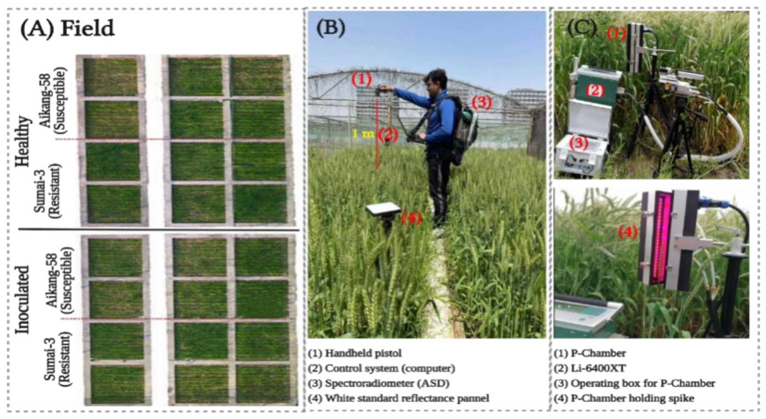
Figure 1. Illustration of applied instruments at canopy scale in field experiment: (A) Field view (B) hyperspectral reflectance data acquisition and (C) photosynthesis rate (Pn) measurement of wheat spikes.
Remotesensing 14 02784 g001
Figure 2. Workflow of the study.
Remotesensing 14 02784 g002
Figure 3. Dynamics of wheat canopy disease variation at different days after inoculation in both wheat growing seasons (2020 and 2021).
Remotesensing 14 02784 g003
Figure 4. Dynamics of wheat canopy net photosynthesis variation at different disease severity percentages after inoculation in the wheat growing season of 2020, where blue asterisks mark the statistical significance between healthy and diseased samples and error bars represent variations within replication.
Remotesensing 14 02784 g004
Figure 5. Correlation scalograms constituted from wavelet coefficients of canopy dataset (9 and 16 DAI) measured in 2019 (A,B) and 2020 (C,D). Finally, common features (E) from both years for spectral bands. The X-axis denotes spectral wavebands of range (400–2400 nm and Y-axis are the wavelet scales from 2 to 8. The grayscales’ higher brightness represents the high correlation with disease and vice versa. The orange color (AD) highlights the top 5% most strong correlation, while (E) highlights intersected values (to interpret colored references in given figure legends, the reader is referred to consult the article’s web version).
Remotesensing 14 02784 g005
Figure 6. Illustration of workflow for spectral indices development. (A): Continuous wavelet analysis (CWT)-based selected five spectral wavelengths (R)—spectral bands—are used as input. (B): All possible normalized two features combination-based indices are developed. (C): All developed or calculated indices are fed to random forest-recursive feature elimination (RF-RFE) to check the most significant indices for fusarium head blight (FHB) detection or classification. (D): Based on classification performance RF-RFE rank indices using variable importance score (VIP), here two most sensitive and robust indices are shown (to interpret colored references in given figure legends, the reader is referred to consult the article’s web version).
Remotesensing 14 02784 g006
Figure 7. Comparison of average classification accuracy (ACA) of newly developed indices; WFCI1~WFCI2: wheat fusarium canopy indices for selected vegetation indices (VIs); NDVI: normalized difference vegetation index; PSNDa~PSNDb~PSNDb: pigment specific normalized difference indices; SIPI: structure-intensive pigment index; LIC1: Lichtenthaler index; RR4: Simple Ratio; NDWI: normalized difference water index at all machine learning classifiers (MLC), where (A,B) shows the ACA of 2020 and 2021, respectively.
Remotesensing 14 02784 g007
Figure 8. Comparison of classification accuracy (CA) of different machine learning classifiers (MLC): (A) CA of different MLC for newly developed canopy indices in 2020 and 2021 and an average of both years. (B) CA of different MLC for conventional spectral indices.
Remotesensing 14 02784 g008
Figure 9. Illustration of univariate quantitative relationship among spectral vegetation indices (VIs) and disease severity (DS): (AJ) Right Y-axis (feature data points — green circles) and X-axis (disease severity) are scatter plots of corresponding features using datasets of the first year (2020), on the basis of which disease estimation model equations (Eqs)—plotting linear curve in univariate simple regression—are developed; (AJ) left Y-axis (estimated DS — blue triangles) and X-axis (observed DS) are 1:1 cross-validations of Eqs for each corresponding feature, using datasets of the second year (2021). (A): Normalized difference vegetation index (NDVI); (B): structure-intensive pigment index (SIPI); (C): Lichtenthaler index (LIC1); (D): Simple Ratio (RR4); (E): pigment specific normalized difference index (PSNDc); (F): normalized difference water index (NDWI); (G,H): pigment specific normalized difference indices (PSNDa and PSNDb); (I,J): wheat fusarium canopy indices (WFCI1 and WFCI2) (the reader is referred to the article’s web version for interpreting—colored references in figure legends).
Remotesensing 14 02784 g009
Figure 10. Illustration of the multivariate quantitative relationship between newly developed indices: wheat fusarium canopy indices (WFCI1 and WFCI2) and disease severity (DS) using the dataset of the first year (2020) for calibration (circles) and dataset of the second year (2021) for validation (triangles) with (A) random forest regression (RFR), (B) support vector machine regression (SVMR) and (C) Knn regression (KnnR) (the reader is referred to the article’s web version for interpreting—colored references in figure legends).
Remotesensing 14 02784 g010
Figure 11. The averaged spectral signatures from two years of experiments. Healthy: reflectance at the day of inoculation; DAI: days after inoculation; (A) reflectance spectra at different disease infection severities; (B) 400–100 nm wavelength at different DAI; (C) 1451–1770 nm at different DAI; (D) 2000–2400 nm at different DAI (to interpret colored references in given figure legends, the reader is referred to consult the article’s web version.).
Remotesensing 14 02784 g011
Table 1. The list of the highly correlated top 8 VIs for each wheat season that are calculated through the pooled dataset of 2020 and 2021 independently.
RankHighly Correlated for 2020RHighly Correlated for 2021RAverageR
1WFCI10.95WFCI10.85WFCI10.90
2WFCI20.94WFCI20.84WFCI20.89
3NDVI−0.94PSNDc−0.83PSNDb−0.88
4PSNDa−0.94SIPI−0.82NDVI−0.87
5PSNDb−0.94PSNDb−0.81PSNDa−0.87
6LIC1−0.94NDWI−0.81PSNDc−0.87
7PSNDc−0.91RR40.81LIC1−0.87
8SIPI−0.91NDVI−0.80SIPI−0.86
9RR40.91PSNDa−0.80NDWI−0.86
10NDWI−0.90LIC1−0.80RR40.86
Table 2. Classification accuracy of the newly developed and conventional spectral indices employing different machine learning classifiers.
Overall Classification Accuracy (%)
This Classification Accuracy (CA) Is for Test Data Set (Train = 70, Test = 30)
Year 2020 2021
DAI58101215681017
DP9.7310.781824.1230.128.2112.4119.3428.13
(A)Knn66.6766.67100.0100.0100.073.3377.7888.89100.0
WFCI1RF83.33100.0100.0100.0100.073.3377.78100.0100.0
SVM66.6787.50100.0100.0100.073.3388.89100.0100.0
NN83.3383.33100.0100.0100.080.0088.8988.89100.0
Xgboost66.6783.33100.0100.0100.086.6788.8988.89100.0
(B)Knn50.0066.67100.0100.0100.070.5966.6787.50100.0
WFCI2RF83.3383.33100.0100.0100.073.3388.8990.00100.0
SVM66.67100.0100.0100.0100.073.33100.088.89100.0
NN66.6783.33100.0100.0100.073.3388.8988.89100.0
Xgboost66.6783.33100.0100.0100.073.3388.89100.0100.0
(C)Knn33.3366.6783.3383.33100.060.0055.5688.89100.0
NDVIRF33.3366.67100.066.67100.053.3366.6777.78100.0
SVM66.6766.6783.3383.33100.053.3355.5688.89100.0
NN50.0066.67100.083.33100.053.3366.6788.89100.0
Xgboost66.6766.67100.083.33100.066.6766.6777.78100.0
(D)Knn33.3350.0066.6783.33100.050.0066.6780.00100.0
PSNDaRF66.6766.6766.6766.67100.066.6780.0077.78100.0
SVM50.0066.6760.0083.33100.050.0066.6788.89100.0
NN50.0066.6783.3383.33100.066.6788.8988.89100.0
Xgboost50.0066.6783.3383.33100.066.6766.6777.78100.0
(E)Knn50.0066.6783.3383.3388.8850.0077.7877.7888.88
PSNDbRF50.0050.0083.3383.3388.8873.3377.7877.7888.88
SVM50.0066.6783.3383.3388.8873.3377.7888.8988.88
NN50.0066.6783.3383.3388.8850.0077.7877.7888.88
Xgboost50.0066.6783.3383.3388.8850.0088.8988.8988.88
DAI is the days after inoculation, DS is the disease percentage or severity, Knn is K-nearest neighbor classifier, RF is the random forest classifier, SVM is the support vector machine classifier, NN is the neural net classifier and Xgboost is the extreme gradient boost classifier.
Publisher’s Note: MDPI stays neutral with regard to jurisdictional claims in published maps and institutional affiliations.