
Efficient Detection of Earthquake−Triggered Landslides Based on U−Net++: An Example of the 2018 Hokkaido Eastern Iburi (Japan) Mw = 6.6 Earthquake


Abstract
:1. Introduction
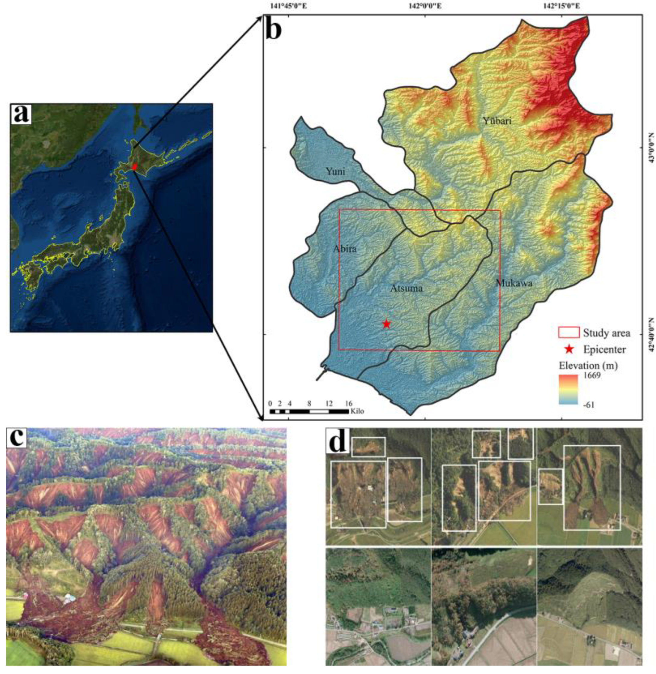
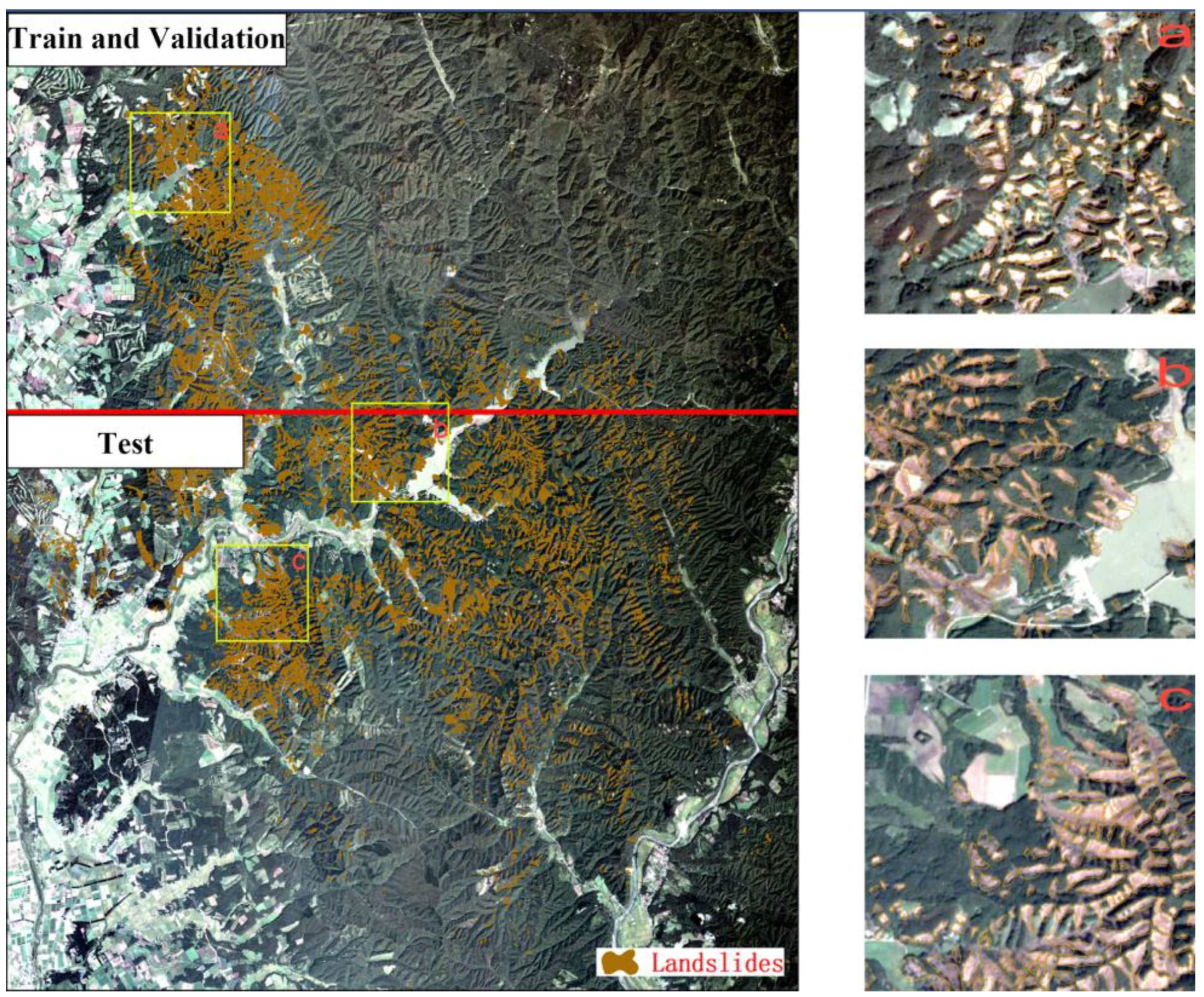
2. Study Area
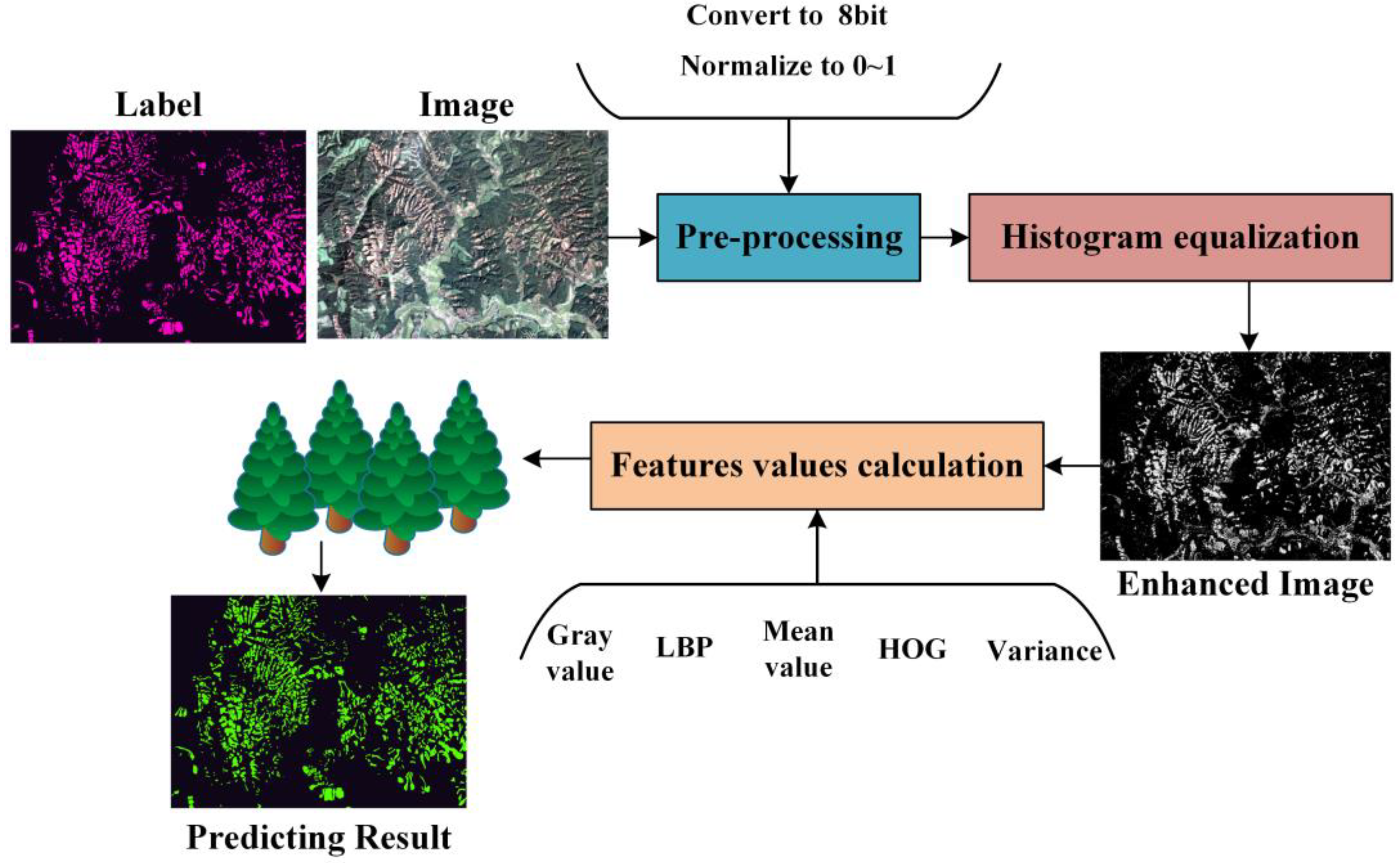
3. Dataset and Pre−Processing
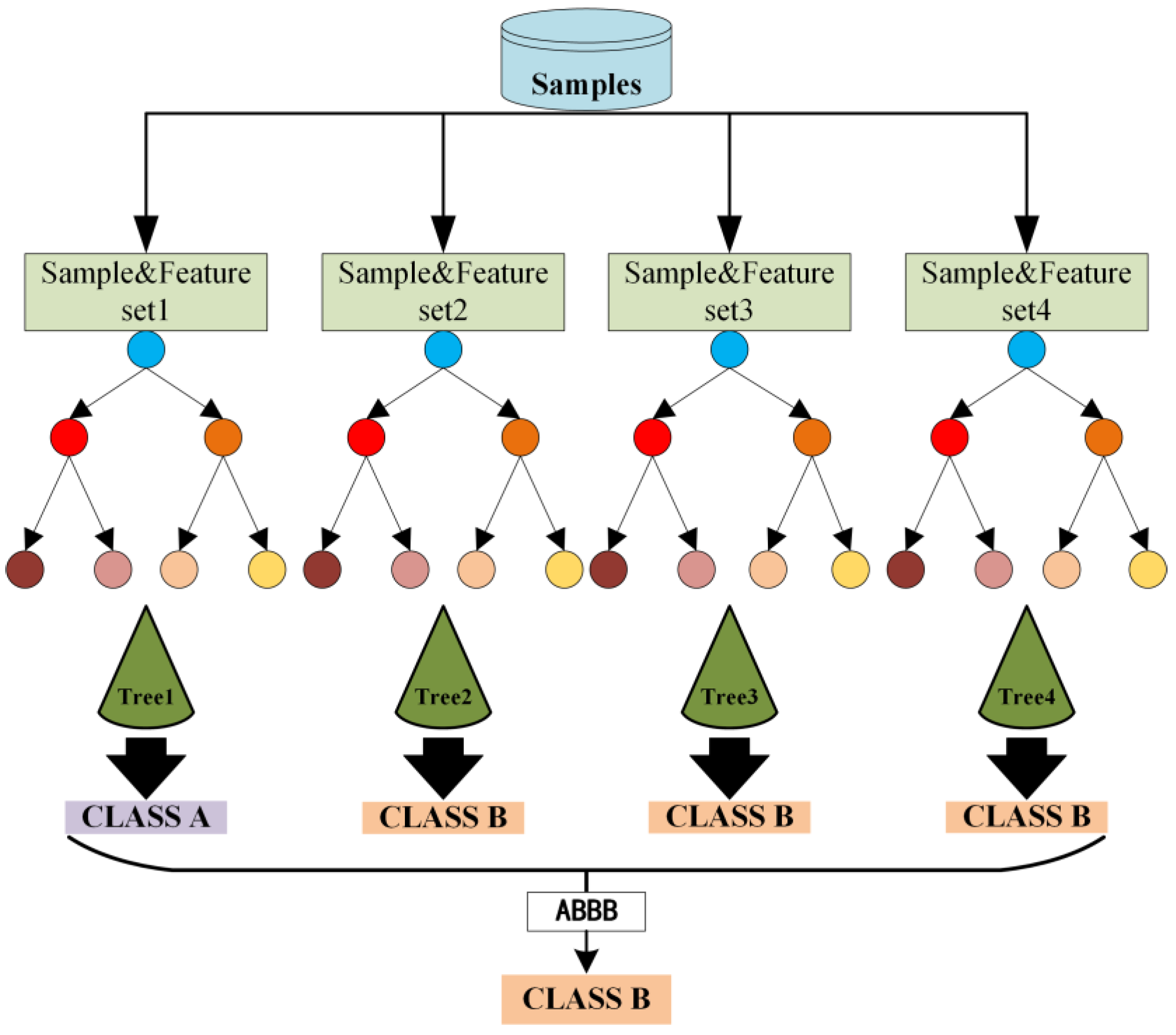
4. Random Forest Algorithm
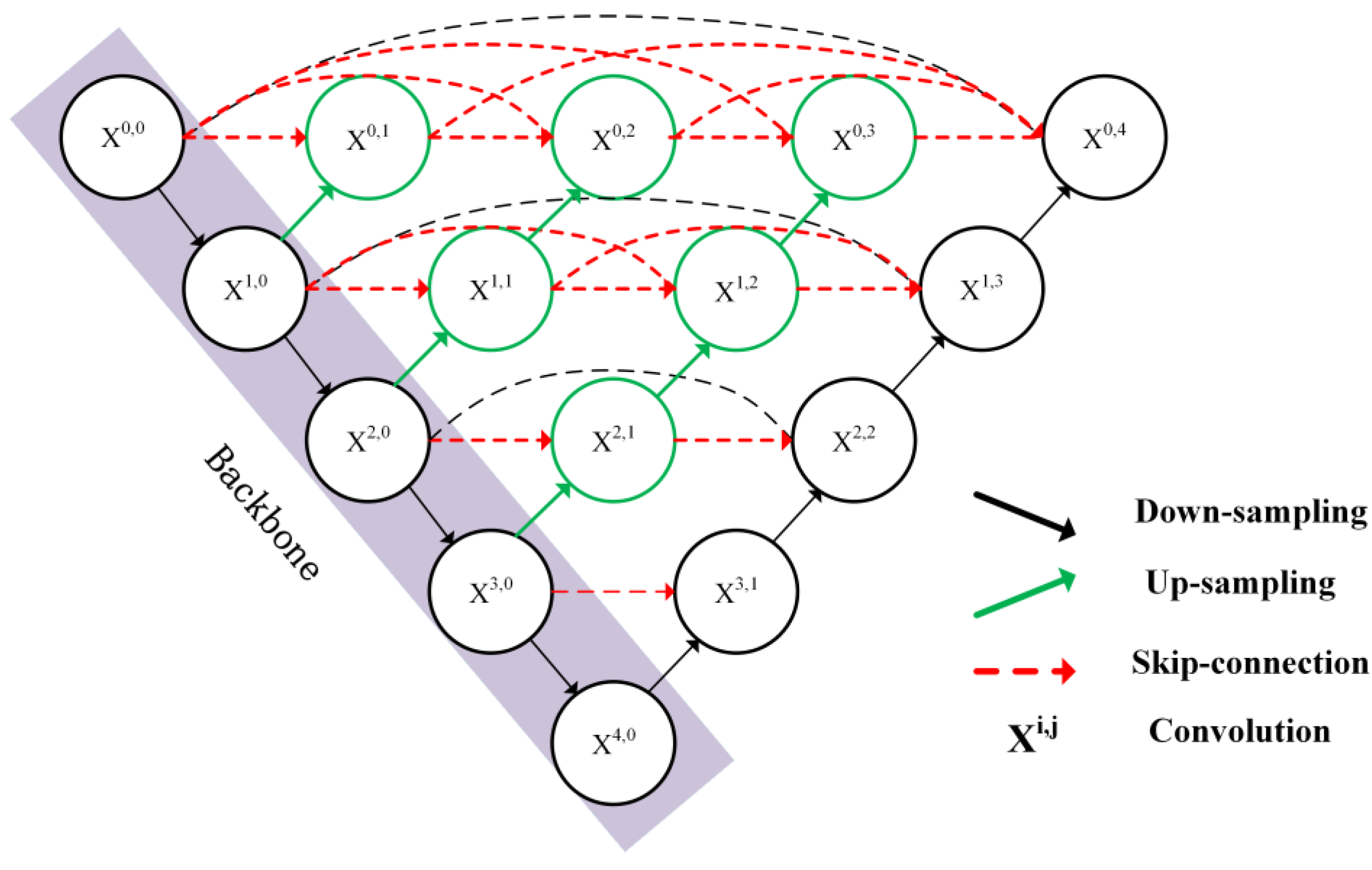
5. U−Net++ and ResNet50
6. Experimental Process
7. Evaluation of Performance
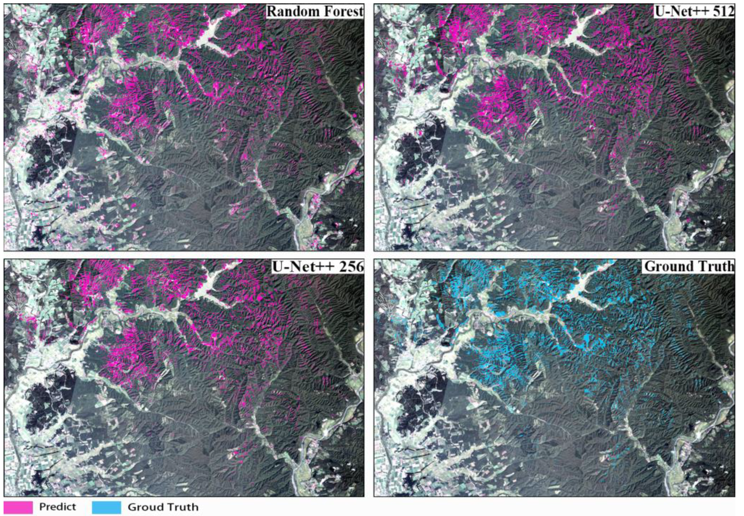
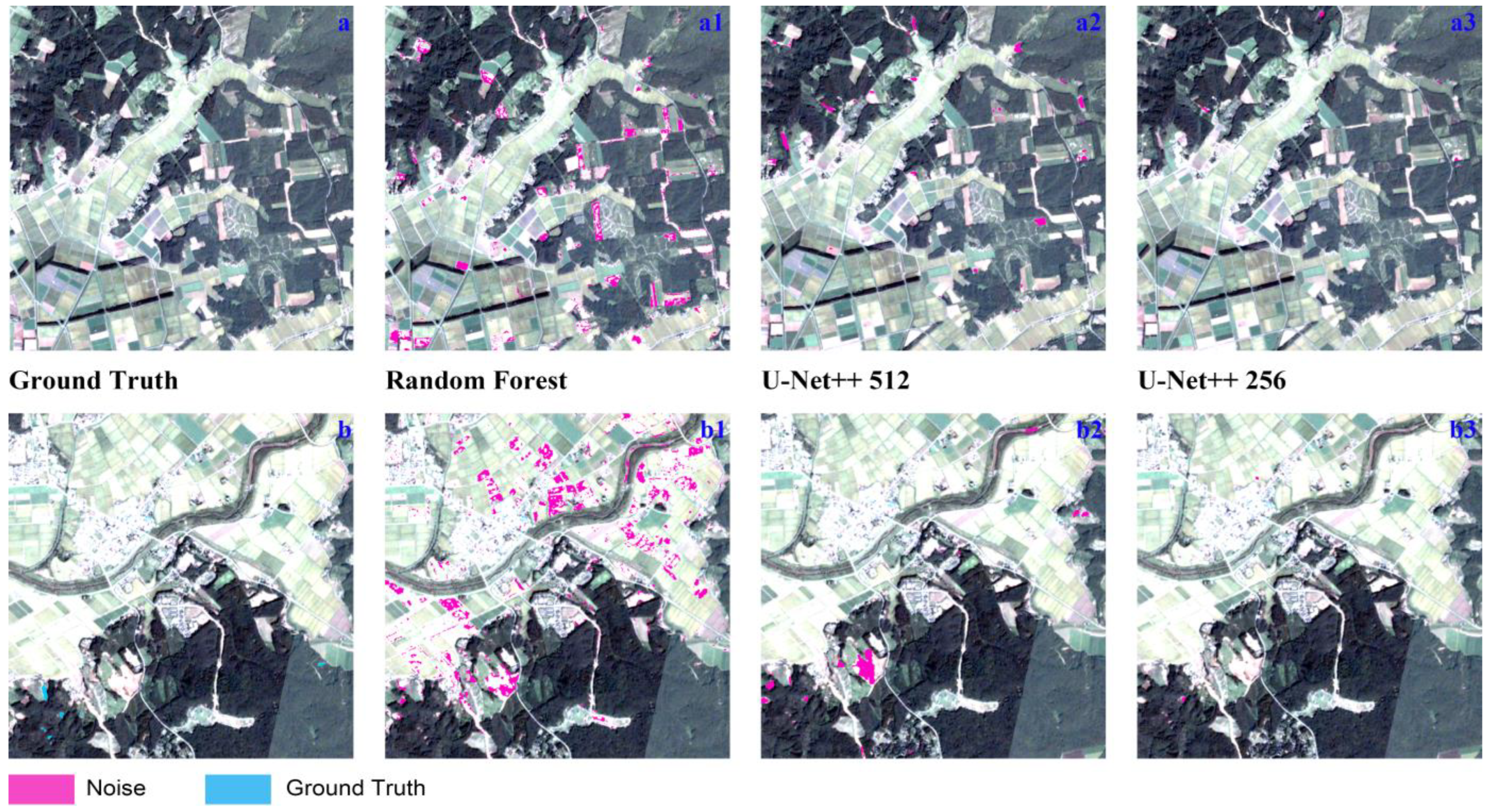
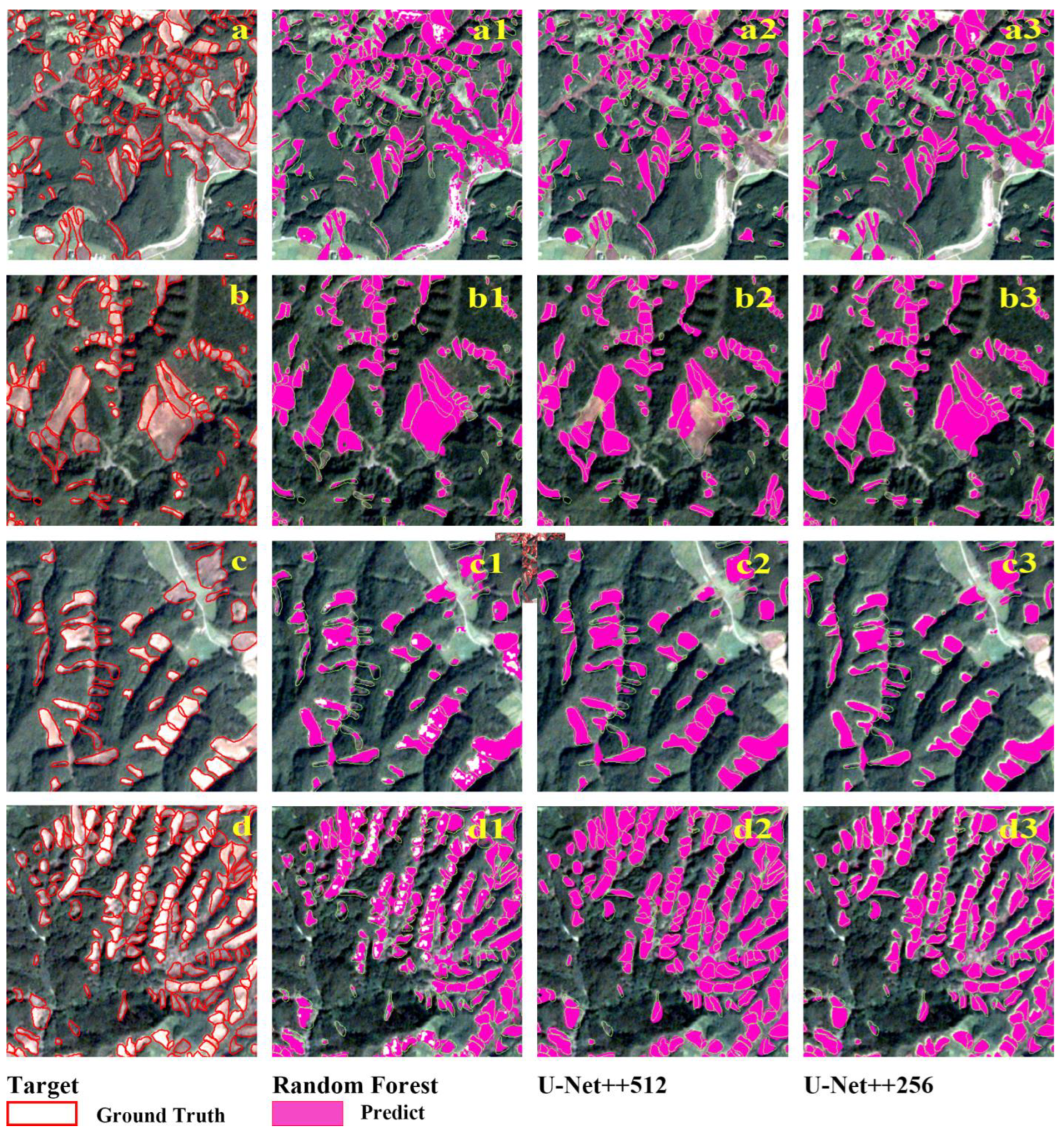
8. Results and Evaluation
9. Discussion
9.1. Model Comparison
9.2. Result Analysis
9.3. Comparison with Previous Work
9.4. Generalization Analysis
9.5. Advantages and Limits
- The image size used in U−Net++ is fixed, and the multi−scale and multi−source remote sensing images are not taken into consideration for extracting more abundant information.
- The high performance of U−Net++ requires the expense of a significant amount of time, and the training speed depends on the computer hardware.
- Although only 1/3 parts of the samples were used in the training stage, the data augmentation was conducted on the dataset to ensure that there were enough datasets for learning, increasing the overhead of GPU.
- Previous studies have shown that size has a non−negligible impact on the DL−based model [44]. In this work, the impact of different sample sizes on U−Net++ is not discussed.
- The quality of the results obtained by the proposed model in preparing the earthquake−triggered landslide susceptibility map is not discussed further.
10. Conclusions
Author Contributions
Funding
Data Availability Statement
Acknowledgments
Conflicts of Interest
References
- Zhu, S.; Shi, Y.; Lu, M.; Xie, F. Dynamic mechanisms of earthquake−triggered landslides. China Earth Sci. 2013, 56, 1769–1779. [Google Scholar] [CrossRef]
- David, K. Keffer. Landslides caused by earthquakes. GSA Bulletin. 1984, 95, 406–421. [Google Scholar] [CrossRef]
- Yao, X.; Xu, C.; Dai, F.; Zhang, Y. Contribution of strata lithology and slope gradient to landslides triggered by Wenchuan Ms 8 earthquake, Sichuan, China. Geol. Bull. China 2009, 28, 1156–1162. [Google Scholar]
- Xu, C. Catalogue of landslides and the amount of slope material lost due to the 2013 Lushan earthquake in China. In Proceedings of the Annual Meeting of Chinese Geoscience Union (2014), Beijing, China, 20–23 October 2014. [Google Scholar]
- Huang, Y.; Xu, C.; Zhang, X.; Xue, C.; Wang, S. An updated database and spatial distribution of landslides triggered by the Milin, Tibet Mw6.4 Earthquake of 18 November 2017. Earth Sci. 2021, 32, 1069–1078. [Google Scholar] [CrossRef]
- Harp, E.L.; Keefer, D.K.; Sato, H.P.; Yagi, H. Landslide inventories: The essential part of seismic landslide hazard analyses. Eng. Geology. 2011, 122, 9–21. [Google Scholar] [CrossRef]
- Bacha, A.S.; Shafique, M.; van der Werff, H. Landslide inventory and susceptibility modelling using geospatial tools, in Hunza−Nagar valley, northern Pakistan. Mt. Sci. 2018, 15, 1354–1370. [Google Scholar] [CrossRef]
- Peng, L.; Xu, S.; Mei, J.; Su, F. Earthquake−induced landslide recognition using high-resolution remote sensing images. J. Remote Sens. 2017, 21, 509–518. [Google Scholar] [CrossRef]
- Chigira, M.; Yagi, H. Geological and geomorphological characteristics of landslides triggered by the 2004 Mid Niigta prefecture earthquake in Japan. Eng. Geology 2006, 82, 202–2210. [Google Scholar] [CrossRef]
- Nichol, J.; Wong, M. Satellite remote sensing for detailed landslide inventories using change detection and image fusion. Int. J. Remote Sens. 2005, 26, 1913–1926. [Google Scholar] [CrossRef]
- Hang, H.; Tung, H.; Hoa, P.; Phuong, N.; Phong, T.; Costache, R.; Nguyen, H.; Amiri, M.; Le, H.; Le, H.; et al. Spatial prediction of landslides along National Highway−6, Hoa Binh province, Vietnam using novel hybrid models. Geocarto Int. 2021, 1–26. [Google Scholar] [CrossRef]
- Lei, T.; Zhang, Y.; Lv, Z.; Li, S.; Liu, S.; Nandi, A. Landslide Inventory Mapping from Bitemporal Images Using Deep Convolutional Neural Networks. IEEE Geosci. Remote. Sens. Lett. 2019, 16, 982–986. [Google Scholar] [CrossRef]
- Zhang, D.; Wu, Z.; Li, J.; Jiang, Y. An overview on earthquake−induced landslide research. J. Geomech. 2013, 19, 225–241. [Google Scholar]
- Saba, S.B.; van der Meijde, M.; van der Werff, H. Spatiotemporal landslide detection for the 2005 Kashmir earthquake region. Geomorphology 2010, 124, 17–25. [Google Scholar] [CrossRef]
- Gorum, T.; Fan, X.; van Westen Cees, J.; Huang, R.; Xu, Q.; Tang, C.; Wang, G. Distribution pattern of earthquake−induced landslides triggered by the 12 May 2008 Wenchuan earthquake. Geomorphology 2011, 133, 152–167. [Google Scholar] [CrossRef]
- Sato, H.P.; Hasegawa, H.; Fujiwara, S.; Tobita, M.; Koarai, M.; Une, H.; Iwahashi, J. Interpretation of landslide distribution triggered by the 2005 Northern Pakistan earthquake using SPOT−5 imagery. Landslides 2007, 4, 113–122. [Google Scholar] [CrossRef]
- Lu, D.; Mausel, P.; Brondízio, E.; Moran, E. Change detection techniques. Int. J. Remote Sens. 2004, 25, 2365–2401. [Google Scholar] [CrossRef]
- Li, S.; Hua, H. Automatic recognition of landslides based on change detection. In Proceedings of the International Symposium on Photoelectronic Detection and Imaging 2009: Advances in Imaging Detectors and Applications, Beijing, China, 17–19 June 2009; Volume 7384. [Google Scholar] [CrossRef]
- Li, Z.; Shi, W.; Myint, S.; Lu, P.; Wang, Q. Semi−automated landslide inventory mapping from bitemporal aerial photographs using change detection and level set method. Remote Sens. Environ. 2016, 175, 215–230. [Google Scholar] [CrossRef]
- Plank, S.; Twele, A.; Martinis, S. Landslide Mapping in Vegetated Areas Using Change Detection Based on Optical and Polarimetric SAR Data. Remote Sens. 2016, 8, 307. [Google Scholar] [CrossRef] [Green Version]
- Rodriguez, K.; Weissel, J.; Kim, Y. Classification of landslide surfaces using fully polarimetric SAR: Examples from Taiwan. IEEE Geosci. Remote Sens. Lett. 2002, 5, 2918–2920. [Google Scholar] [CrossRef]
- Yonezawa, C.; Watanabe, M.; Saito, G. Polarimetric Decomposition Analysis of ALOS PALSAR Observation Data before and after a Landslide Event. Remote Sens. 2012, 4, 2314–2328. [Google Scholar] [CrossRef] [Green Version]
- Shibayama, T.; Yamaguchi, Y.; Yamada, H. Polarimetric Scattering Properties of Landslides in Forested Areas and the Dependence on the Local Incidence Angle. Remote Sens. 2015, 7, 15424–15442. [Google Scholar] [CrossRef] [Green Version]
- Raspini, F.; Ciampalini, A.; Del Conte, S.; Lombardi, L.; Nocentini, M.; Gigli, G.; Ferretti, A.; Casagli, N. Exploitation of Amplitude and Phase of Satellite SAR Images for Landslide Mapping: The Case of Montescaglioso (South Italy). Remote Sens. 2015, 7, 14576–14596. [Google Scholar] [CrossRef] [Green Version]
- Mountrakis, G.; Im, J.; Ogole, C. Support vector machines in remote sensing: A review. ISPRS J. Photogramm. Remote Sens. 2011, 66, 247–259. [Google Scholar] [CrossRef]
- Myles, A.J.; Feudale, R.N.; Liu, Y.; Woody, N.A.; Brown, S.D. An introduction to decision tree modeling. J. Chemom. A J. Chemom. Soc. 2004, 18, 275–285. [Google Scholar] [CrossRef]
- Breiman, L. Random forests. Mach. Learn. 2001, 45, 5–32. [Google Scholar] [CrossRef] [Green Version]
- Atkinson, P.M.; Tatnall, A.R.L. Introduction neural networks in remote sensing. Int J Remote Sens. 1997, 18, 699–709. [Google Scholar] [CrossRef]
- Maxwell, A.E.; Warner, T.A.; Fang, F. Implementation of machine-learning classification in remote sensing: An applied review. Int. J. Remote Sens. 2018, 39, 2784–2817. [Google Scholar] [CrossRef] [Green Version]
- Lary, D.; Alavi, A.; Gandomi, S.; Walker, A. Machine learning in geosciences and remote sensing. Geosci. Front. 2016, 7, 3–10. [Google Scholar] [CrossRef] [Green Version]
- Mahesh, B. Machine Learning Algorithms—A Review. Int. J. Sci. Res. 2019, 9, 381–386. [Google Scholar] [CrossRef]
- Zhou, X.; Wen, H.; Zhang, Y.; Xu, J.; Zhang, W. Landslide susceptibility mapping using hybrid random forest with GeoDetector and RFE for factor optimization. Geosci. Front. 2021, 12, 101211. [Google Scholar] [CrossRef]
- Chen, T.; Trinder, J.C.; Niu, R. Object−Oriented Landslide Mapping Using ZY−3 Satellite Imagery, Random Forest and Mathematical Morphology, for the Three−Gorges Reservoir, China. Remote Sens. 2017, 9, 333. [Google Scholar] [CrossRef] [Green Version]
- Ghorbanzadeh, O.; Blaschke, T.; Gholamnia, K.; Meena, S.R.; Tiede, D.; Aryal, J. Evaluation of Different Machine Learning Methods and Deep−Learning Convolutional Neural Networks for Landslide Detection. Remote Sens. 2019, 11, 196. [Google Scholar] [CrossRef] [Green Version]
- Zhu, X.; Tuia, D.; Mou, L.; Xia, G.; Zhang, L.; Xu, F.; Fraundorfer, F. Deep Learning in Remote Sensing: A Comprehensive Review and List of Resources. IEEE Geosci. Remote Sens. Lett. 2017, 5, 8–36. [Google Scholar] [CrossRef] [Green Version]
- Milletari, F.; Ahmadi, S.; Kroll, C.; Plate, K.; Rozanski, V.; Maiostre, M.; Levin, J.; Dietrich, O.; Ertl-Wagner, B.; Bötzel, K.; et al. Hough−CNN: Deep learning for segmentation of deep brain regions in MRI and ultrasound. Comput. Vis. Image Underst. 2017, 164, 92–102. [Google Scholar] [CrossRef] [Green Version]
- Hesamian, M.; Jia, W.; He, X.; Kennedy, P. Deep Learning Techniques for Medical Image Segmentation: Achievements and Challenges. Digit. Imaging 2019, 32, 582–596. [Google Scholar] [CrossRef] [Green Version]
- Shahri, A.; Moud, F. Landslide susceptibility mapping using hybridized block modular intelligence model. Bull. Eng. Geol. Environ. 2021, 80, 267–284. [Google Scholar] [CrossRef]
- Ji, S.; Yu, D.; Shen, C.; Li, W.; Xu, Q. Landslide detection from an open satellite imagery and digital elevation model dataset using attention boosted convolutional neural networks. Landslides 2020, 17, 1337–1352. [Google Scholar] [CrossRef]
- Shi, W.; Zhang, M.; Ke, H.; Fang, X.; Zhan, Z.; Chen, S. Landslide Recognition by Deep Convolutional Neural Network and Change Detection. IEEE Trans. Geosci. Remote Sens. 2021, 59, 4654–4672. [Google Scholar] [CrossRef]
- Sameen, M.; Pradhan, B. Landslide Detection Using Residual Networks and the Fusion of Spectral and Topographic Information. IEEE Access. 2019, 7, 114363–114373. [Google Scholar] [CrossRef]
- Ronneberger, O.; Fischer, P.; Brox, T. U−Net: Convolutional Networks for Biomedical Image Segmentation. In Proceedings of the 18th Medical Image Computing and Computer−Assisted Intervention (MICCAI 2015), Munich, Germany, 5–9 October 2015; pp. 234–241. [Google Scholar] [CrossRef]
- Soares, L.; Dias, H.; Grohmann, C. Landslide Segmentation with U−Net: Evaluating Different Sampling Methods and Patch Sizes. arXiv 2020, arXiv:2007.06672. [Google Scholar] [CrossRef]
- Zhang, P.; Xu, C.; Ma, S.; Shao, X.; Tian, Y.; Wen, B. Automatic Extraction of Seismic Landslides in Large Areas with Complex Environments Based on Deep Learning: An Example of the 2018 Iburi Earthquake, Japan. Remote Sens. 2020, 12, 3992. [Google Scholar] [CrossRef]
- Qi, W.; Wei, M.; Yang, W.; Xu, C.; Ma, C. Automatic Mapping of Landslides by the ResU−Net. Remote Sens. 2020, 12, 487. [Google Scholar] [CrossRef]
- Yi, Y.; Zhang, W. A New Deep−Learning−Based Approach for Earthquake−Triggered Landslide Detection from Single−Temporal RapidEye Satellite Imagery. IEEE J. Sel. Top. Appl. Earth Obs. Remote Sens. 2020, 13, 6166–6176. [Google Scholar] [CrossRef]
- Su, Z.; Chow, J.; Tan, p.; Wu, J.; Ho, Y.; Wang, Y. Deep convolutional neural network–based pixel−wise landslide inventory mapping. Landslides 2021, 18, 1421–1443. [Google Scholar] [CrossRef]
- Ghorbanzadeh, O.; Crivellari, A.; Ghamisi, P.; Shahabi, H.; Blaschke, T. A comprehensive transferability evaluation of U−Net and ResU−Net for landslide detection from Sentinel−2 data (case study areas from Taiwan, China, and Japan). Sci. Rep. 2021, 11, 14629. [Google Scholar] [CrossRef] [PubMed]
- Prakash, N.; Manconi, A.; Loew, S. Mapping Landslides on EO Data: Performance of Deep Learning Models vs. Traditional Machine Learning Models. Remote Sens. 2020, 12, 346. [Google Scholar] [CrossRef] [Green Version]
- Ghorbanzadeh, O.; Gholamnia, K.; Ghamisi, P. The application of ResU−net and OBIA for landslide detection from multi−temporal sentinel−2 images. Big Earth Data 2022, 1–26. [Google Scholar] [CrossRef]
- Ghorbanzadeh, O.; Shahabi, H.; Crivellari, A.; Homayouni, S.; Blaschke, T.; Ghamisi, P. Landslide detection using deep learning and object−based image analysis. Landslides 2022, 19, 929–939. [Google Scholar] [CrossRef]
- Rahimzad, M.; Homayouni, S.; Alizadeh Naeini, A.; Nadi, S. An Efficient Multi−Sensor Remote Sensing Image Clustering in Urban Areas via Boosted Convolutional Autoencoder (BCAE). Remote Sens. 2021, 13, 2501. [Google Scholar] [CrossRef]
- Shahabi, H.; Rahimzad, M.; Tavakkoli Piralilou, S.; Ghorbanzadeh, O.; Homayouni, S.; Blaschke, T.; Lim, S.; Ghamisi, P. Unsupervised Deep Learning for Landslide Detection from Multispectral Sentinel−2 Imagery. Remote Sens. 2021, 13, 4698. [Google Scholar] [CrossRef]
- Zhou, Z.; Rahman Siddiquee, M.; Tajbakhsh, N.; Liang, J. UNet++: A Nested U−Net Architecture for Medical Image Segmentation. In Proceedings of the 4th International Workshop, DLMIA 2018, and 8th International Workshop, ML−CDS 2018, Held in Conjunction with MICCAI 2018, Granada, Spain, 20 September 2018; pp. 3–11. [Google Scholar] [CrossRef]
- Yamagishi, H.; Ito, Y.; Kawamura, M. Characteristics of deep−seated landslides of Hokkaido: Analyses of a database of landslides of Hokkaido, Japan. Environ. Eng. Geosci. 2002, 8, 35–46. [Google Scholar] [CrossRef]
- Yamagishi, H.; Yamazaki, F. Landslides by the 2018 Hokkaido Iburi−Tobu Earthquake on September 6. Landslides 2018, 15, 2521–2524. [Google Scholar] [CrossRef] [Green Version]
- Zhang, S.; Li, R.; Wang, F.; Iio, K. Characteristics of landslides triggered by the 2018 Hokkaido Eastern Iburi earthquake, Northern Japan. Landslides 2019, 16, 1691–1708. [Google Scholar] [CrossRef]
- Shao, X.; Ma, S.; Xu, C.; Zhang, P.; Wen, B.; Tian, Y.; Zhou, Q.; Cui, Y. Planet Image−Based Inventorying and Machine Learning−Based Susceptibility Mapping for the Landslides Triggered by the 2018 Mw6.6 Tomakomai, Japan Earthquake. Remote Sens. 2019, 11, 978. [Google Scholar] [CrossRef] [Green Version]
- Pal, M. Random Forest classifier for remote sensing classification. Int J Remote Sens. 2005, 26, 217–222. [Google Scholar] [CrossRef]
- Jaiswal, J.; Samikannu, R. Application of Random Forest Algorithm on Feature Subset Selection and Classification and Regression. In Proceedings of the World Congress on Computing and Communication Technologies (WCCCT,2017), Tiruchirappalli, India, 2–4 February 2017; pp. 65–68. [Google Scholar] [CrossRef]
- Dalal, N.; Triggs, B. Histograms of oriented gradients for human detection. In Proceedings of the 2005 IEEE Computer Society Conference on Computer Vision and Pattern Recognition (CVPR’05), San Diego, CA, USA, 20–25 June 2015; pp. 886–893. [Google Scholar] [CrossRef] [Green Version]
- Ojala, T.; Pietikäinen, M.; Harwood, D. A comparative study of texture measures with classification based on featured distributions. Pattern Recognit. 1996, 29, 51–59. [Google Scholar] [CrossRef]
- Santurkar, S.; Tsipras, D.; Ilyas, A.; Madry, A. How does batch normalization help optimization? arXiv 2018, arXiv:1805.11604. [Google Scholar] [CrossRef]
- Lu, L.; Shin, Y.; Su, Y.; Karniadakis, G.E. Dying relu and initialization: Theory and numerical examples. arXiv 2019, arXiv:1903.06733. [Google Scholar] [CrossRef]
- Milletari, F.; Navab, N.; Ahmadi, S. V−Net: Fully Convolutional Neural Networks for Volumetric Medical Image Segmentation. In Proceedings of the 2016 Fourth International Conference on 3D Vision (3DV), Stanford, CA, USA, 25–28 October 2016; pp. 565–571. [Google Scholar] [CrossRef] [Green Version]
- Garcia−Garcia, A.; Orts−Escolano, S.; Oprea, S.; Villena−Martinez, V.; Garcia−Rodriguez, J. A review on deep learning techniques applied to semantic segmentation. arXiv 2017, arXiv:1704.06857. [Google Scholar] [CrossRef]
- Susmaga, R. Confusion matrix visualization. In Intelligent Information Processing and Web Mining; Springer: Berlin/Heidelberg, Germany, 2004; Volume 25, pp. 107–116. [Google Scholar] [CrossRef]
- Razavi, S.; Jakeman, A.; Saltelli, A.; Prieur, C.; Iooss, B.; Borgonovo, E.; Plischke, E.; Piano, S.L.; Iwanaga, T.; Becker, W.; et al. The future of sensitivity analysis: An essential discipline for systems modeling and policy support. Environ. Model. Softw. 2021, 137, 104954. [Google Scholar] [CrossRef]
- Saltelli, A.; Aleksankina, K.; Becker, W.; Fennell, P.; Ferretti, F.; Holst, N.; Li, S.; Wu, Q. Why so many published sensitivity analyses are false: A systematic review of sensitivity analysis practices. Environ. Model. Softw. 2019, 114, 29–39. [Google Scholar] [CrossRef]
- Asheghi, R.; Hosseini, S.A.; Saneie, M.; Shahri, A.A. Updating the neural network sediment load models using different sensitivity analysis methods: A regional application. J. Hydroinform. 2020, 22, 562–577. [Google Scholar] [CrossRef] [Green Version]
- Yakubovskiy, P.; Segmentation Models Pytorch. GitHub Repository. 2020. Available online: https://github.com/qubvel/segmentation_models.pytorch (accessed on 11 March 2022).


| Prediction Truth 1 | Prediction False 0 | |
|---|---|---|
| Ground Truth 1 | TP | FN |
| Ground False 0 | FP | TN |
| Type | Accuracy | Precision | Recall | F1−Score | Kappa | IoU |
|---|---|---|---|---|---|---|
| RF | 96.03 | 62.81 | 64.03 | 63.42 | 61.32 | 46.43 |
| U−Net++512 | 96.88 | 71.92 | 68.84 | 70.35 | 68.70 | 54.26 |
| Compared to RF | ↑0.85 | ↑9.11 | ↑4.81 | ↑6.93 | ↑7.38 | ↑7.83 |
| U−Net++256 | 97.38 | 75.26 | 76.36 | 75.80 | 74.42 | 61.04 |
| Compared to RF | ↑1.35 | ↑12.45 | ↑12.33 | ↑12.38 | ↑13.10 | ↑14.61 |
| Compared to 512 | ↑0.50 | ↑3.34 | ↑7.52 | ↑5.45 | ↑5.72 | ↑6.78 |
| Type | TP | FN | FP | TN | Total |
|---|---|---|---|---|---|
| RF | 1,480,314 | 831,425 | 876,568 | 39,819,693 | 43,008,000 |
| U−Net++512 | 1,591,441 | 720,298 | 621,240 | 40,075,021 | |
| U−Net++256 | 1,765,174 | 546,565 | 580,304 | 40,115,957 |
| Depth | Precision | Recall | F1−Score | Kappa | IoU | Time |
|---|---|---|---|---|---|---|
| 3 | 76.33 | 76.11 | 76.22 | 74.87 | 61.58 | 6.7 h |
| 4 | 73.95 | 75.44 | 74.69 | 73.24 | 59.60 | 10 h |
| 5 | 75.26 | 76.36 | 75.80 | 74.42 | 61.04 | 13.3 h |
| Type | Accuracy | Precision | Recall | F1−Score | Kappa | IoU |
|---|---|---|---|---|---|---|
| U−Net++256 | 95.86 | 89.60 | 92.30 | 90.93 | 88.25 | 83.37 |
Publisher’s Note: MDPI stays neutral with regard to jurisdictional claims in published maps and institutional affiliations. |
© 2022 by the authors. Licensee MDPI, Basel, Switzerland. This article is an open access article distributed under the terms and conditions of the Creative Commons Attribution (CC BY) license (https://creativecommons.org/licenses/by/4.0/).
Share and Cite
Yang, Z.; Xu, C. Efficient Detection of Earthquake−Triggered Landslides Based on U−Net++: An Example of the 2018 Hokkaido Eastern Iburi (Japan) Mw = 6.6 Earthquake. Remote Sens. 2022, 14, 2826. https://doi.org/10.3390/rs14122826
Yang Z, Xu C. Efficient Detection of Earthquake−Triggered Landslides Based on U−Net++: An Example of the 2018 Hokkaido Eastern Iburi (Japan) Mw = 6.6 Earthquake. Remote Sensing. 2022; 14(12):2826. https://doi.org/10.3390/rs14122826
Chicago/Turabian StyleYang, Zhiqiang, and Chong Xu. 2022. "Efficient Detection of Earthquake−Triggered Landslides Based on U−Net++: An Example of the 2018 Hokkaido Eastern Iburi (Japan) Mw = 6.6 Earthquake" Remote Sensing 14, no. 12: 2826. https://doi.org/10.3390/rs14122826