
Sparse Approximation of the Precision Matrices for the Wide-Swath Altimeters

US Naval Research Laboratory, Stennis Space Center, MS 39522, USA
Remote Sens. 2022, 14(12), 2827; https://doi.org/10.3390/rs14122827
Submission received: 23 May 2022
/
Revised: 10 June 2022
/
Accepted: 11 June 2022
/
Published: 13 June 2022
(This article belongs to the Special Issue Remote Sensing Technology for New Ocean and Seafloor Monitoring)
Abstract
:The upcoming technology of wide-swath altimetry from space will deliver a large volume of data on the ocean surface at unprecedentedly high spatial resolution. These data are contaminated by errors caused by the uncertainties in the geometry and orientation of the on-board interferometer and environmental conditions, such as sea surface roughness and atmospheric state. Being highly correlated along and across the swath, these errors present a certain challenge for accurate processing in operational data assimilation centers. In particular, the error covariance matrix of the Surface Water and Ocean Topography (SWOT) mission may contain trillions of elements for a transoceanic swath segment at kilometer resolution, and this makes its handling a computationally prohibitive task. Analysis presented here shows, however, that the SWOT precision matrix and its symmetric square root can be efficiently approximated by a sparse block-diagonal matrix within an accuracy of a few per cent. A series of observational system experiments with simulated data shows that such approximation comes at the expense of a relatively minor reduction in the assimilation accuracy, and, therefore, could be useful in operational systems targeted at the retrieval of submesoscale variability of the ocean surface.
1. Introduction
The upcoming Surface Water and Ocean Topography (SWOT, [1,2]) and Coastal and Ocean Measurement with Precise and Innovative Radar Altimeter (COMPIRA, [3]) missions are planned to deliver high resolution maps of the ocean surface topography using radar interferometers. This new type of observations of the sea surface height (SSH) will deliver gridded data along 100–150 km wide swaths at kilometer resolution. To achieve the target SSH accuracy of a few centimeters, this new remote sensing technology requires taking into the account multiple observation errors of instrumental and environmental origin that are spatially correlated.
Dealing with spatial correlations of swath altimetry errors in presents a certain challenge for the operational data assimilation systems, mostly because of the huge dimension of the respective error covariance matrices. As an example, a 3000 km long swath segment will contain on order of a million of spatially correlated observations whose error covariance matrix will have elements, and, therefore will be computationally expensive to handle.
In preparation for the SWOT mission, the Jet Propulsion Laboratory (JPL) developed the observation error covariance model [2,4] which served as a basis for numerous experiments aimed at assessing both the added value of the mission in monitoring the global ocean (e.g., [5,6,7,8,9]) and at dealing with spatial correlations of the errors contaminating SWOT observations (e.g., [10,11,12]).
In particular, ref. [10] proposes employing high-order differential operators to penalize the grid-scale components along the swath, while [11,13] explore a method of removing SSH errors caused by the uncertainties in interferometer geometry and orientation (hereinafter referred to as geometric and orientation errors, GOEs). In their recent study, Yaremchuk et al. [12] proposed a separable approximation to the GOE covariance matrix and its inverse, which provide significant computational savings at the expense of a slight modification of the along-swath error spectra of the JPL model. Heuristic sparse approximations of the inverse error covariance for the SWOT mission were also proposed in the earlier studies by Ruggiero et al. [7] and Yaremchuk et al. [14].
In a more general perspective, the problem of introducing non-diagonal observation error covariances into data assimilation systems requires an efficient algorithm for statistically consistent normalization of the innovations (i.e., multiplication of the innovations by the inverse square root of the respective observational error covariance matrix ). This necessity is evident from from the relationship between the model increment and the normalized innovation vector :
Here, is the observation operator projecting the background model state on observations , is its linearization in the vicinity of , is the diagonal matrix of the background standard deviations, is the respective correlation matrix, is the identity matrix, and the superscript denotes transposition.
In this study, we explore a possibility of approximating the SWOT precision matrix and its symmetric square root by sparse matrices. Such approximations facilitate computationally efficient performance of the data assimilation systems in both dual (Equation (1)) and primal (state space) formulations.
The paper is organized as follows. In the next section we analyze the structure of the SWOT error covariance matrix and propose approximations reducing it to the block-diagonal form that is also separable in the across- and along-swath directions. In Section 3 the numerical testing methodology of these approximations is described and the respective errors are computed, as well as the results of observation system simulation experiments with several versions of the precision matrix approximations with different accuracy. The findings are summarized and discussed in Section 4.
2. Structure of the Wide-Swath Error Covariance Matrix
The JPL error covariance model [4], developed in preparation for the SWOT mission, is represented by the sum of three major constituents, associated with the errors caused by uncertainties in the geometry and orientation of the on-board interferometer, uncertainties in the environmental conditions (state of the atmosphere and ocean waves), and the intrinsic noise of the Ka-band Radar Interferometer (KaRIn) itself:
Here, , and denote the respective (GOE, environmental and KaRIn) covariance matrices in the above-mentioned order. We denote the KaRIn noise error covariance by to distinguish its diagonal positive-definite structure, whereas the other two components are generally rank-deficient (positive semi-definite) and non-diagonal (i.e., have significant error correlations in the across- and along-swath directions). In the following, these directions are denoted by respectively x and y, while all the matrices operating in these directions will be subscripted accordingly.
2.1. Separable Approximation of the GOE Covariance Matrix
The general structure of the GOE model [4,12] is given by
where p enumerates the four GOE components associated with uncertainties in the roll, phase, baseline length and timing of the on-board interferometer, ⊗ denotes the tensor product, , are the respective across-swath covariance matrices, are the along-swath power spectra shown in the left panel of Figure 1, and , denote, respectively, the Fourier transformation matrix in the along-swath direction and its inverse.
Similarity in the shape of the spectra in Figure 1 allows to rescale them and introduce their “optimal mean” spectral shape shown in Figure 1 by the thick black line. After plugging the inverses of the spectral rescaling factors into , the GOE covariance can be approximated by the matrix of the form
where now denote the across-swath covariances rescaled by . As it was shown in [12], the error of such approximation does not exceed several per cent, which is likely to be well within the modeling uncertainty of the original spectra shown in Figure 1. Further reduction can be achieved by performing singular value decomposition of the sum in the rhs of Equation (4):
where is the matrix of the orthonormal eigenmodes shown in the right panel of Figure 1, and is the diagonal matrix of the respective eigenvalues. Equation (5) can also be rewritten in the more compact form
with and . This representation allows one to obtain the pseudoinverse of by computing the reciprocals of the diagonal entries of .
It is also worthwhile to note that the approximation (5) also implies separability of the SWOT covariance (2) in the across- and along-swath directions if and can be represented in the form and . Separability is a useful property from the computational point of view, as it allows one to easily compute and parallelize the action of , and on a vector employing operations only involving small ( and ) matrices operating in the across- and along-swath directions.
Separable approximations could be made under realistic assumptions about environmental factors affecting the structure of these matrices. First, the diagonal elements of depend on the significant wave height (SWH) underneath the satellite [4], and one may assume that SWH varies on spatial scales of the dominant atmospheric disturbances (≃500 km) that are much larger than the typical half-width (50 km) of the swath. In this case, spatial variation of the diagonal elements of could be approximated by the product of the across-swath structure function corresponding to the mean SWH over the swath segment, and a slowly varying function in the along-swath direction. So, neglecting SWH variation across the swath appears to be a reasonably good approximation, at least for relatively short swath segments in the open ocean. Similarly, the structure of is also defined by the scales of atmospheric disturbances in the water vapor and aerosol content, so a separable representation of (e.g., using a Gaussian kernel in the spectral space) appears to be a reasonable option.
2.2. Sparse Approximation of the Precision Matrix and Its Square Root
In what follows, we neglect in Equation (2), as the magnitude of the respective noise appears to be several times smaller than the magnitude of KaRIn and GOE constituents, at least in the two-beam radiometer configuration [4]. Assuming separability of the KaRIn noise error covariance matrix, consider separable approximation of the precision matrix . Combining the representation (6) with the Woodbury identity, and rewriting the precision matrix in the form
consider a polynomial expansion of the matrix inverse in the right-hand side. The latter is valid if one of the matrices under the inversion sign is sufficiently small compared to the other, so that the inverse of their sum could be represented by a convergent Taylor series. Inspection of the rms magnitudes of the KaRIn noise errors [4] indicates that within a realistic range (1 to 8 m) of the SWH conditions, the typical magnitude of (1–2 cm) is considerably (3–5 times) smaller than the magnitude of the sum of GOEs , so we could consider the second term in the sum to dominate, and rearrange the inverted matrix in (7) by rewriting it in the form:
where is the identity matrix and
is the symmetric square root of .
The matrix inverse in the rhs of Equation (8) can be expanded in the convergent series if all the eigenvalues of the expansion matrix do not exceed 1. Because of the matrix separability,
the eigenvalues can be inexpensively obtained by decomposition of the respective and matrices in the rhs of (10) given their definition in the rhs of (9).
The eigenvalues of the expansion matrix in the lhs of (10) are then obtained as a tensor product of two vectors containing eigenvalues of the matrices in the rhs of (10) operating in the across- and along-swath directions. Results of these computations are shown in the left panel of Figure 2 for a 512 km long swath segment at 2 km resolution. It is seen that for SWH values less than 6 m, just a few terms of the Taylor expansion provide a good approximation of the precision matrix as the largest eigenvalue does not exceed 0.22.
It is also noteworthy that since we are interested in retrieval of submesoscale SSH variability with spatial frequencies above 10 km (wavelengths below the half-width of the satellite swath, which is 50–60 km), the respective part of the along-swath precision matrix spectrum is nearly flat (Figure 1) and contributes more than 90% to the total precision (inverse error variance). Therefore, the white noise could be a reasonable approximation of the along-swath spectrum if we are particularly interested in retrieving the submesoscale components of the SSH variability. What is more important, this approximation sparsifies the SWOT precision matrix estimate reducing Equation (7) to the block-diagonal form:
In the case of constant SWH, in the rhs of Equation (11) turns into the identity matrix, and all the blocks become identical (see Appendix A for more details). Equation (11) demonstrates that the precision matrix can be decoupled in the along- and across-swath directions if the inverse of the along-swath GOE spectrum is approximated by the white noise. Inspection of Figure 1 shows that such approximation is rather accurate, because the inverse of the optimized spectrum is nearly flat for wavelengths below 50 km ( km) and quickly falls down at longer wavelengths, which contribute less than 1% to the wavenumber integral.
To summarize, these analytical considerations indicate that block-diagonal approximations of and may have a reasonable accuracy, especially for the purpose of retrieving submesocale SSH variability within the swath.
Although Equation (11) provides a simple way to obtain the diagonal blocks of the precision matrix, it still requires first to get reliable approximations of [12], and . A more general and accurate way of doing this in practice, is to minimize the Frobenius norm of the following expressions in the space of symmetric block-diagonal matrices :
with the structure of given by the JPL error model, and Equation (3) in particular. Note that due to the block-diagonal form of the target matrix , these problems can be executed in parallel for each of the blocks, each having a rather moderate size of the control vector which is equal to the number of elements in the upper triangle of the across-swath covariance matrix. Similar approach is routinely used in computing the approximate sparse preconditioners for iterative solvers (e.g., [15]).
3. Numerical Tests
3.1. Methodology
To test the proposed approach, we conducted a series of twin data assimilation experiments with a 512 km long swath segment defined on rectangular grid with km resolution (Figure 3). The true (reconstructed) SSH field was defined on the same grid and computed as a single realization of a Gaussian field with zero mean, the decorrelation scale of km and the amplitude a of 2 cm shown in the top panel of Figure 3.
To simulate the data assimilation process, two 100-member ensembles of the “model fields” and “SWOT observations” were created, and then the estimates of the true state were reconstructed for each pair of the ensemble members. The model fields were generated by contaminating with realizations of the background noise (model errors) characterized by the decorrelation scale km and the amplitude of 1 cm. The Gaussian random fields used for generating both the true sea surface height field and the background noise were defined by the covariance function
where is the Laplacian operator (e.g., [16,17]) on the model grid with Neumann boundary conditions.
As mentioned above, the information on the true field was provided by the simulated model fields and SWOT “observations” at 2 km resolution. Realizations of the respective error fields were computed by
where is the normally distributed 2d field, and , are the square roots of the background (14) and SWOT (2) error covariances. Two realizations of the “modelled” and “observed” fields are shown in the middle and bottom panels of Figure 3.
Given 100 realizations of the “model output” and “observations”, three hundred data assimilation experiments using Equation (1) were conducted to compute the optimal correction to the model field. These experiments employed three types of representation (diagonal, block-diagonal and exact) for the inverse square root of in Equation (1). The first two approximations were obtained by the respective restrictions of the sparsity patterns for in Equation (13).
To quantify the results of assimilation experiments, the mean relative deviations e of the analyses from the true state were computed
as well as their ensemble means .
3.2. Results
The block-diagonal approximation of was computed under the condition of constant SWH over the swath ( in Equation (11)) currently available in the SWOT simulator. At 2 km resolution of the SWOT grid, this problem had a moderate size of and was not computationally expensive. To check the block-diagonal approximation quality, we also computed the exact precision matrix and a series of its sparsifications . The latter were obtained by setting to zero all the elements of whose absolute value was less than a given threshold . Results of these computations as a function of the sparsity parameter , (here N is the number of non-zero elements of a matrix), are presented in the left panel of Figure 2. The approximation errors were defined by the Frobenius norm ratio . The plot gives an evidence that; (a) the block-diagonal approximation of is an order in magnitude better than just taking the diagonal of , and (b) provides an accuracy of roughly 2%, which is nearly identical to accuracy obtained by the above described sparsification method when is equal to its block-diagonal value of .
For the symmetric square root of the precision matrix, the errors are somewhat larger, but still remain within the reasonably accurate limits of 2–2.7%, even for larger SWH values that magnify the KaRIn noise quite significantly. Results of these preliminary computations are assembled in Table 1. It should be also noted that the SWOT covariance matrix does not have a similar sparse approximation as the respective errors were found to be quite close to a hundred per cent, and ranged within 0.98–0.997 for the tested swath configuration.
To estimate the impact of assimilating SWOT data, we computed the increments in Equation (1) for the 100-member ensembles of realizations of the background and simulated SWOT error fields. A couple of ensemble members of the background and observed fields are shown in the middle and bottom panels of Figure 3. In each of the ensembles of the assimilation solutions, three forms of the square root of the SWOT precision matrix were used: the exact symmetric square root of the inverse covariance, its block-diagonal and diagonal approximations. The latter was obtained by inverting the square root of the ensemble-based estimate of diag(R) derived from the SWOT simulator output by squaring the ensemble members in each grid point and averaging the result.
An example of such a twin-data assimilation experiment is shown in Figure 4 for an ensemble member with moderate sea surface roughness SWH = 2 m.
To assess the overall impact of the block-diagonal approximation on the accuracy of submesoscale retrievals from SWOT observations, we conducted a series of numerical experiments with sea surface roughness parameter increasing from 2 to 8 m. Results of these experiments are assembled in Table 2.
The major tendencies are the general increase of the analysis error e, and reduction of its range (the difference between lines 1 and 3) with the increasing SWH. It is also remarkable that the analysis errors obtained with the diagonal approximation of (line 3) decrease from 0.37 to 0.31 with the increase of the significant wave height from 2 to 8 m. This can be explained by the growth of the KaRIn noise contribution to the error budget
shown in the bottom line of Table 2. Indeed, rougher seas reduce the overall accuracy of the SSH retrieval at submesoscale (upper line in Table 2) and at the same time increase the covariance matrix diagonal , improving the quality of the diagonal approximation for the precision matrix (third line). The growing diagonal dominance of the SWOT covariance matrix reduces the importance of taking the spatial error covariances into the account with the increase of the sea surface roughness.
Quantitatively, improvement in the accuracy of submesoscale retrievals using the block-diagonal approximation (computed as the ratio of the respective errors) degrades from 1.6 to 1.3 with the growth of SWH from 2 to 7 m. These numbers indicate utility of the proposed approximation of the SWOT precision matrix in a wide range of sea surface roughness conditions.
4. Conclusions and Discussion
Analysis of the structure of the SWOT error covariance matrix has shown a possibility to approximate its inverse square root by a sparse matrix within the accuracy of a few per cent. The approximation was successfully tested in a series of twin data assimilation experiments, and demonstrated a capability to improve the assimilation accuracy 1.3–1.6 times compared to a simple diagonal approximation of the error covariance. The improvement is observed over the range of significant sea surface heights of 2–8 m, and could be even better for calmer seas.
The analytical analysis of precision matrix and its square root indicate that their block-diagonal approximations are more accurate for retrieval of the SSH structures with typical wavelengths below the swath half-width (scales less than 20 km). This makes the proposed approximation technique especially suitable for multi-scale data assimilation (e.g., [18,19]) at its final stage, after correction of the larger-scale (mesoscale) structures of the model state. Furthermore, since the typical magnitude of SSH perturbations at submesoscale (2–4 cm, [20]) is comparable to (and often less than) SWOT errors [4], statistically consistent treatment of the spatial structure of the observation error covariances becomes especially important in the analysis and assimilation of the SWOT data at the wavelengths below 50 km. Comparison of the analysis error fields (shown in middle and bottom panels of Figure 4) provides a particular demonstration of the necessity to properly take into account spatial correlations of the observational errors within the swath.
In this study, we did not consider the contribution of uncertainties in atmospheric water content and nadir altimeter observations on the overall accuracy of the SSH reconstruction. Preliminary consideration indicates that the magnitude of is several times smaller than the contributions from KaRIn noise and , at least in the two-beam radiometer configuration, which removes the linear trend of the vapor-related path delay across the swath [4]. The relatively small magnitude of may provide an asymptotic guidance for updating the sparsity pattern of the precision matrix by taking the wet atmosphere corrections into the account. Similar asymptotic techniques can be possibly used for treatment of spatial variations of the SWH field and dry atmosphere corrections. These modifications are planned to be implemented in the JPL model in the near future.
Comparison of the first and second rows in Table 2 shows that there is still a considerable room for improving the block-diagonal approximation of the sparsity pattern for the precision matrices. Solutions to this challenging problem could be further developed by the joint analysis of real data from the forthcoming satellite missions and ensemble simulations of the ocean surface topography by state-of-the-art numerical models. In particular, the specific structure of the wide-swath altimetry error covariances may be exploited to improve the sparsity patterns of the precision matrices by the deep learning techniques (e.g., [21,22]) and other methods involving neural networks. Extensive literature (e.g., [23,24,25,26]) also exists on purely algebraic methods of approximating the inverse covariances. These methods do not explicitly take into account the specific structure of the covariance model, as it was done in the present study. Of particular interest are applications of the modified Cholesky decomposition [24], under the sparsifying assumption of conditional independence of the observation errors beyond a given localization scale in the along-swath direction. This approach is suitable for efficient parallelization [25] of the precision matrix approximations specifically tailored for retrieving SSH variability at submesoscale.
In the SWOT application, one may think of combining the above-mentioned methods to obtain accurate and computationally efficient approximations of the precision matrices. The presented study could be considered as another step towards this ultimate goal.
Funding
This research was funded by the ONR (Office of Naval Research) project number 73-6C95-02.
Conflicts of Interest
The author declares no conflict of interest.
Appendix A. White Noise Approximation of the Along-Swath Covariance
Omitting the along-swath index y for brevity, taking into account the Fourier transform property , and substituting the definition into the mth term of the inverse matrix expansion in the along-swath direction yields
Plugging the approximation into (A1) reduces this relationship to
References
- Durand, M.; Fu, L.L.; Lettenemaier, D.; Alsdorf, D.; Rodriguers, E.; Esteban-Fernandez, D. The surface water and ocean topography mission: Observing terrestrial surface water and oceanic submesoscale eddies. Proc. IEEE 2010, 98, 766–779. [Google Scholar] [CrossRef]
- Esteban-Fernandez, D. SWOT Project: Mission Performance and Error Budget. Revision A. NASA/JPL Tech. Rep. JPL D-79084. 2013. Available online: http://https://ieeexplore.ieee.org/document/8517385 (accessed on 12 June 2022).
- Ito, N.; Uematsu, A.; Yajima, Y.; Isoguchi, O. A Japanese new altimetry mission COMPIRA—Towards high temporal and spatial sampling of sea surface height. AGU Fall Meet. 2014, OS34B-05. Available online: https://agu.confex.com/agu/fm14/webprogram/Paper21766.html (accessed on 12 June 2022).
- Gaultier, L.; Ubelmann, C.; Fu, L.-L. SWOT Simulator Documentation; Tech. Rep. 2.3.0; Jet Propulsion Laboratory, CalTech: Pasadena, CA, USA, 2017.
- Gaultier, L.; Ubelmann, C.; Fu, L.-L. The challenge of using future SWOT data for oceanic field reconstruction. J. Atm. Ocean. Technol. 2016, 33, 119–126. [Google Scholar] [CrossRef]
- Li, Z.; Wang, J.; Fu, L.-L. An observing system simulation experiment for ocean state estimation to assess the performance of the SWOT mission: Part 1—A twin experiment. J. Geophys. Res. Ocean. 2019, 124, 4838–4855. [Google Scholar] [CrossRef]
- Ruggiero, G.A.; Cosme, E.; Brankart, J.M.; Le Sommer, J.; Ubelmann, C. An efficient way to account for observation error correlations in the assimilation of data from the future SWOT high-resolution altimeter mission. J. Atmos. Ocean. Technol. 2016, 33, 2755–2768. [Google Scholar] [CrossRef]
- Ubelmann, C.; Klein, E.; Fu, L.L. Dynamic interpolation of sea surface height and potential applications for future high-resolution altimetry mapping. J. Atmos. Ocean. Technol. 2015, 32, 177–184. [Google Scholar] [CrossRef] [Green Version]
- Wang, J.; Fu, L.L.; Qui, B.; Menemenlis, D.; Farrar, J.T.; Chao, Y.; Thompson, A.F.; Flexas, M.M. An observing system simulation experiment for the calibration and validation of the SWOT sea surface height measurement using in situ platforms. J. Atmos. Ocean. Technol. 2018, 35, 281–297. [Google Scholar] [CrossRef]
- Gomez-Navarro, L.; Cosme, E.; Sommer, J.L.; Papadakis, N.; Pascual, A. Development of an image de-noising method in preparation for SWOT satellte mission. Remote Sens. 2020, 12, 734. [Google Scholar] [CrossRef] [Green Version]
- Metref, S.; Cosme, E.; Guillou, F.L.; Sommer, J.L.; Brankart, J.-M.; Verron, J. Wide-swath altimetric satellite data assimilation with correlated error reduction. Front. Mar. Sci. 2020, 6, 822. [Google Scholar] [CrossRef] [Green Version]
- Yaremchuk, M.; D’Addezio, J.; Jacobs, G. Facilitating inversion of the error covariance models for the wide-swath altimeters. Remore Sens. 2020, 12, 1823. [Google Scholar] [CrossRef]
- Metref, S.; Cosme, E.; Sommer, J.L.; Poel, N.; Brankart, J.-M.; Verron, J.; Gomez Navarro, L. Reduction of spatially structured errors in wide-swath altimetric satellite data using data assimilation. Remote Sens. 2019, 11, 1336. [Google Scholar] [CrossRef] [Green Version]
- Yaremchuk, M.; D’Addezio, J.; Panteleev, G.; Jacobs, G. On the approximation of the inverse error covariances of high-resolution altimetry data. Q. J. R. Meteorol. Soc. 2018, 144, 1995–2000. [Google Scholar] [CrossRef]
- Chow, E.; Saad, Y. Approximate inverse preconditioners via sparse-sparse iterations. SIAM J. Sci. Comp. 1998, 19, 995–1023. [Google Scholar] [CrossRef] [Green Version]
- Yaremchuk, M.; Smith, S. On the correlation functions associated with polynomials of the diffusion operator. Q. J. R. Meteorol. Soc. 2011, 137, 1927–1932. [Google Scholar] [CrossRef]
- Yaremchuk, M.; Carrier, M.; Smith, S.; Jacobs, G. Background error correlation modeling with diffusion operators. In Data Assimilation for Atmospheric, Oceanic and Hydrologic Applications; Park, S.K., Xu, L., Eds.; Springer: Berlin/Heidelberg, Germany, 2013; Volume II, pp. 177–203. [Google Scholar] [CrossRef]
- Li, Z.; McWiliams, J.C.; Ide, K.; Farrara, J.D. A multi-scale variational data assimilation scheme: Formulation and illustration. Mon. Wea. Rev. 2015, 143, 3804–3822. [Google Scholar] [CrossRef]
- Souopgui, I.; D’Addezio, J.M.; Rowley, C.; Smith, S.; Jacobs, G.A.; Helber, R.; Yaremchuk, M. Multi-scale assimilation of simulated SWOT observations. Ocean Model. 2020, 154, 101683. [Google Scholar] [CrossRef]
- D’Addezio, J.M.; Jacobs, J.M.G.A.; Yaremchuk, M.; Souopgui, I. Submesoscale eddy vertical covariances and dynamical constraints from high-resolution numerical simulations. J. Phys. Oceanogr. 2020, 50, 1087–1115. [Google Scholar] [CrossRef] [Green Version]
- Raissi, M.; Perdikaris, P.; Karniadakis, G.E. Physics-informed neural networks: A deep learning framework for solving forward and inverse problems involving nonlinear partial differential equations. J. Comp. Phys. 2019, 378, 686–707. [Google Scholar] [CrossRef]
- Tavakkoli, V.; Chedjou, J.C.; Kyamakaya, K. A novel recurrent neural network-based ultra-fast, robust, and scalable solver for inverting a time-varying matrix. Sensors 2019, 19, 4002. [Google Scholar] [CrossRef] [Green Version]
- Chang, C.; Tsay, R.S. Estimation of covariance matrix via the sparse Cholesky factor with the lasso. J. Stat. Plan. Inference 2010, 140, 3858–3873. [Google Scholar] [CrossRef]
- Nino-Ruiz, E.D.; Sandu, A.; Deng, X. An ensemble Kalman filter implementation based on modified Cholesky decomposition for inverse covariance matrix estimation. SIAM J. Sci. Comp. 2018, 40, A867–A886. [Google Scholar] [CrossRef]
- Nino-Ruiz, E.D.; Sandu, A.; Deng, X. A parallel implementation of the ensemble Kalman filter implementation based on modified Cholesky decomposition. J. Comp. Sci. 2019, 36, 100654. [Google Scholar] [CrossRef] [Green Version]
- Zhang, W.; Leng, C. A moving average Cholesky factor model in covariance modeling for longitudinal data. Biometrika 2012, 99, 141–150. [Google Scholar] [CrossRef]
Figure 1.
(Left) Square roots of the four GOE spectral components (gray lines) and their optimized approximation (black). The spectra of baseline dilation and timing errors are reduced by an order in magnitude for better viewing. (Right) orthogonal eigenmodes of the across-swath GOE covariance matrix.
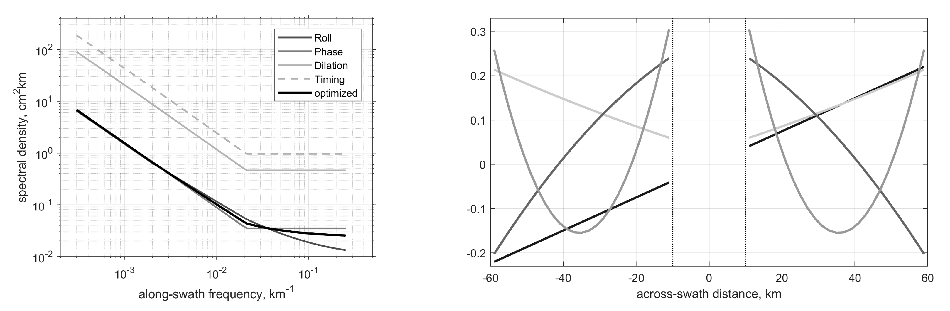
Figure 2.
(Left) Eigenvalues of the expansion matrix in Equation (10) computed for three different values of SWH field at 2 km resolution. (Right) Dependence of the precision matrix approximation error on the fraction of non-zero elements in a matrix. Consecutive (from left to right) dots along the graph correspond to two-time reduction of the threshold value eliminating small matrix elements to obtain an approximation. Thin vertical line corresponds to sparsity of the block-diagonal approximation. Diamond and asterisk mark approximation errors obtained, respectively, by inverting the diagonal of , and keeping only block-diagonal elements of the precision matrix.
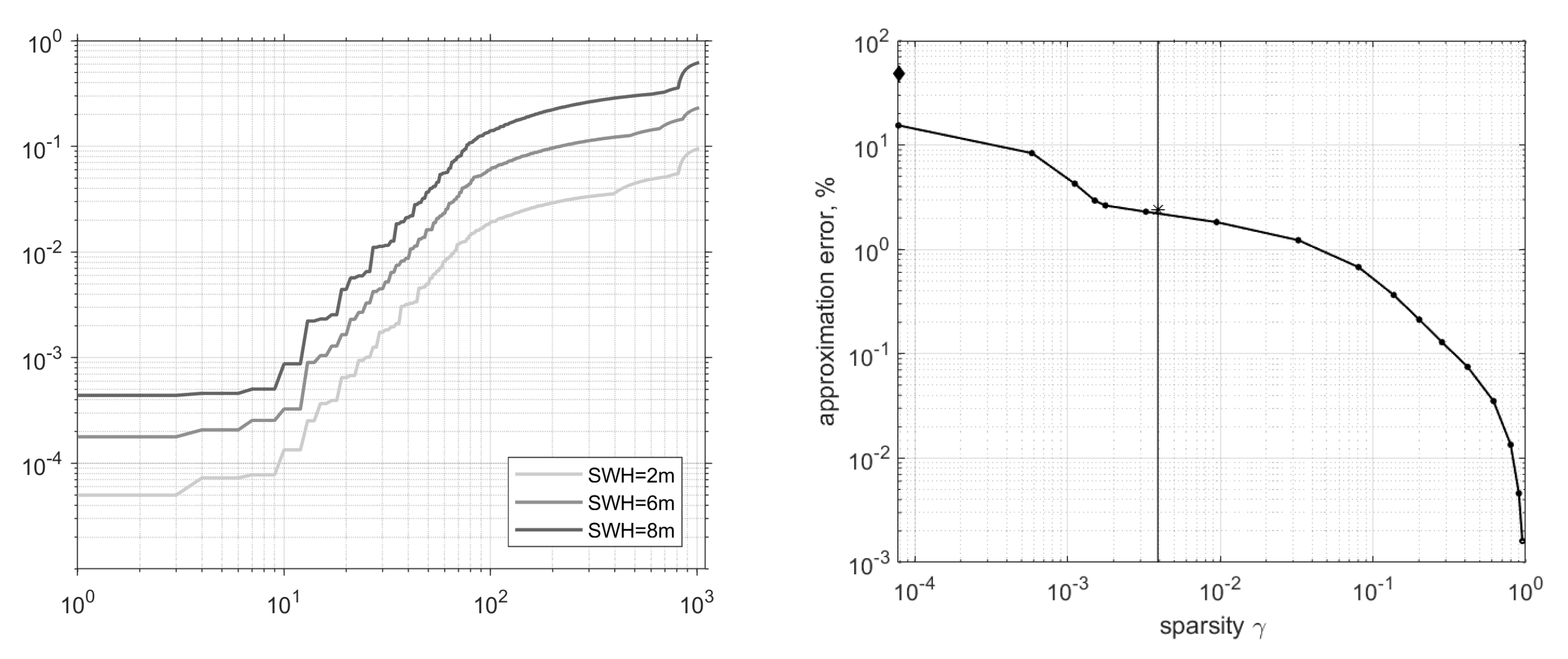
Figure 3.
The true (being reconstructed) SSH field (top), and random realizations of the model background (middle) and observed (bottom) fields. Locations of the simulated SWOT observations are shown by black dots. SSH values are in centimeters.
Figure 3.
The true (being reconstructed) SSH field (top), and random realizations of the model background (middle) and observed (bottom) fields. Locations of the simulated SWOT observations are shown by black dots. SSH values are in centimeters.

Figure 4.
The error fields within the swath region obtained after assimilating the ensemble member in Figure 1 using the exact square root of the inverse covariance (top), its block-diagonal approximation (middle), and the diagonal approximation obtained from n samples of the error fields produced by the SWOT simulator (bottom). Relative deviations (swath-averaged, in %) from the true SSH field are shown in the upper right corners. The color bars are in centimeters.


Table 1.
Block-diagonal approximation errors for the SWOT precision matrix and its symmetric square root for various values of the significant sea surface height.
Table 1.
Block-diagonal approximation errors for the SWOT precision matrix and its symmetric square root for various values of the significant sea surface height.
| SWH, m | 2 | 4 | 6 | 7 | 8 |
|---|---|---|---|---|---|
| 0.0188 | 0.0198 | 0.0209 | 0.0221 | 0.0242 | |
| 0.0204 | 0.0215 | 0.0233 | 0.0250 | 0.0267 |
Table 2.
Ensemble-averaged deviations e (Equation (16)) from the true SSH obtained in the assimilation experiments with the exact square root of the precision matrix in the definition of the normalized observation operator in Equation (1) (first line), with its block-diagonal and diagonal approximations shown in the middle. The contribution of the KaRIn noise to the total error covariance (in %) is displayed at the bottom line.
| SWH, m | 2 | 4 | 6 | 7 | 8 |
|---|---|---|---|---|---|
| 0.16 | 0.17 | 0.19 | 0.21 | 0.22 | |
| 0.23 | 0.24 | 0.25 | 0.26 | 0.26 | |
| 0.37 | 0.35 | 0.34 | 0.33 | 0.31 | |
| 0.41 | 0.46 | 0.59 | 0.70 | 0.77 |
Publisher’s Note: MDPI stays neutral with regard to jurisdictional claims in published maps and institutional affiliations. |
© 2022 by the author. Licensee MDPI, Basel, Switzerland. This article is an open access article distributed under the terms and conditions of the Creative Commons Attribution (CC BY) license (https://creativecommons.org/licenses/by/4.0/).
Share and Cite
MDPI and ACS Style
Yaremchuk, M. Sparse Approximation of the Precision Matrices for the Wide-Swath Altimeters. Remote Sens. 2022, 14, 2827. https://doi.org/10.3390/rs14122827
AMA Style
Yaremchuk M. Sparse Approximation of the Precision Matrices for the Wide-Swath Altimeters. Remote Sensing. 2022; 14(12):2827. https://doi.org/10.3390/rs14122827
Chicago/Turabian StyleYaremchuk, Max. 2022. "Sparse Approximation of the Precision Matrices for the Wide-Swath Altimeters" Remote Sensing 14, no. 12: 2827. https://doi.org/10.3390/rs14122827
Note that from the first issue of 2016, this journal uses article numbers instead of page numbers. See further details here.