Article

Phenology–Gross Primary Productivity (GPP) Method for Crop Information Extraction in Areas Sensitive to Non-Point Source Pollution and Its Influence on Pollution Intensity

1
School of Earth Sciences and Engineering, Hohai University, Nanjing 210098, China
2
Aerospace Information Research Institute, Chinese Academy of Sciences, Beijing 100101, China
*
Author to whom correspondence should be addressed.
These authors contributed equally to this work.
Remote Sens. 2022, 14(12), 2833; https://doi.org/10.3390/rs14122833
Submission received: 25 April 2022 / Revised: 6 June 2022 / Accepted: 8 June 2022 / Published: 13 June 2022
(This article belongs to the Section Ecological Remote Sensing)

Abstract

:
The excessive use of pesticides and fertilizers during agricultural production causes water pollution, which is an important type of non-point source pollution (NSP). Large amounts of harmful substances, such as nitrogen and phosphorus, flow into surface water along with farmland runoff, leading to eutrophication and other problems. However, the pollutant discharge capacity of different types of cultivated land varies greatly. Areas sensitive to NSP are areas with rich crop types, large spatial differences in crop growth, and complex planting patterns. These factors can cause different amounts of fertilizer used in and absorbed by the crops to influence the emission intensity of pollutants. NSP intensity mapping can reflect the spatial distribution of lands’ pollutant discharge capacity and it can provide a basis for pollution control. However, when estimating NSP intensity, existing methods generally treat cultivated land as a category and ignore how complex crop conditions impact pollution intensity. Remote sensing technology enables the classification and monitoring of ground objects, which can provide rich geographical data for NSP intensity mapping. In this study, we used a phenology–GPP (gross primary productivity) method to extract the spatial distribution of crops in the Yuecheng reservoir catchment area from Sentinel-2 remote sensing images and the overall accuracy reached 85%. Moderate resolution imaging spectroradiometer (MODIS) GPP data were used to simulate the spatial distribution of crop growth. Finally, a new model that is more suitable for farmland was obtained by combining this large amount of remote sensing data with existing mapping models. The findings from this study highlight the differences in spatial distributions between total nitrogen and total phosphorous; they also provide the means to improve NSP intensity estimations.

Graphical Abstract

1. Introduction

Non-point source pollution (NSP) refers to the environmental pollution without a fixed sewage outlet. The erosion of rainwater causes dissolved or solid pollutants from non-specific locations, along with surface runoff into receiving water, to create eutrophication and other water-based environmental problems. Compared with point source pollution, NSP is more difficult to measure and quantify, so it is also very difficult to study and manage. NSP intensity is used to quantify NSP and it refers to the total amount of pollutants discharged per unit area per unit time. It is related to the overall pollutant concentration. Greater source intensity leads to more serious pollution [1]. The differences of ground object types and geographical environment cause the obvious spatial distribution differences of NSP source intensity. NSP intensity’s spatial expression represents the ability of land in each unit region to pollute the environment, which is highly significant for targeted NSP control and provides an important basis for rationally adjusting ground object types and structures. Farmland areas sensitive to NSP in the agricultural industry mainly comprise areas in which the cultivated land distribution is more complex. The spatial distribution of farmland NSP intensity is easily affected by crop type, crop condition, crop growth cycle, multiple croppings, and other factors. When one or several of these factors show spatial differences, the source intensity also changes. These factors usually influence the emission intensity of pollutants by causing different amounts of fertilizer used in and absorbed by the crops. For example, multiple cropping is widely used in Asia and Africa as a planting mode to improve the utilization efficiency of cultivated land [2]. When multiple cropping is performed in a field, two or more crop types are planted in different seasons of the year, which leads to an increase in the frequency of farmland fertilization. The resulting NSP intensity in this type of crop planting mode differs from the pollution intensity when a single crop is planted in a particular field. In addition, the amounts of fertilizer and growth cycles vary among crop types, which also affect the intensity of NSP [3]. Fertilization standards differ for each type of crop. Each crop’s growing season also affects the location of fertilizer. For example, in areas with both rain and heat, or where more precipitation falls in summer, fertilizer loss is more likely to occur, while in places with less precipitation during winter, fertilizer is more likely to stay in situ, where crops absorb it. Crop growth also partially reflects fertilizer uptake and affects the intensity of NSP [4]. With all other conditions remaining the same, when a crop fixes more organic carbon through photosynthesis, it can grow better, absorb more fertilizer, and leave fewer pollutants in the environment. These complex situations have considerable impacts on the spatial distribution of NSP intensity. To accurately estimate NSP intensity, the accurate extraction of crop information is necessary. However, multiple factors (e.g., rapid changes in environmental conditions, the adjustment of government management policies, changes in market regulation, and farmers’ willingness to report growth conditions) can cause crop configurations to significantly fluctuate over time [5]. National and/or local governments’ regulatory policies cause multiple cropping indexes to continuously fluctuate. Crops’ growing conditions also vary over time. All of these factors make it more challenging to estimate NSP intensity. Overall, this involves two main problems. One is the lack of a mapping model of NSP intensity specifically for farmland that considers complex conditions, while the other is a lack of dynamic spatial and temporal data for finding extensive crop information inside cultivated agricultural land.
For the first problem, thus far, multiple NSP models have emerged in an attempt to provide more accurate pollution estimates. For different research areas, these models have partially solved the problem of NSP and some models are now widely used [6,7,8,9,10,11,12,13,14,15]. However, these models have distinct advantages and disadvantages. For example, some use only a single empirical value for averaging simulations, which leads to low accuracy and difficulty with universal application [16,17,18,19,20,21,22,23,24]. Although some techniques can accurately simulate the process of pollutant generation, they may require many parameters and extensive calculations, thus limiting their application [25,26,27]. The diffuse pollution estimation with a remote sensing (DPeRS) model [28] was developed to apply remote sensing to the estimation of a NSP load by coupling the quantitative remote sensing model and the eco-hydrological process model to adjust for regions without data. Concurrently, the raster pixel was used as the calculation unit to ensure the simulation accuracy and calculation efficiency of the model [29]. Importantly, the DPeRS model cannot be used to calculate NSP loads without the estimation of the NSP intensity. NSP load and NSP intensity are distinct concepts. NSP intensity refers to the emissions of NSP into the environment generated by a specific type of land, while NSP load refers to the emissions generated by a specific type of land (i.e., NSP intensity) through migration and transformation, finally reaching the water supply [1]. Therefore, NSP intensity is an important parameter for calculating pollution load, which has a critical role in management and mitigation efforts. Compared with NSP load, NSP intensity is a more stable physical quantity. However, the current estimation of NSP intensity is based on land-use data [1,29,30,31,32]. With this approach, cultivated land is generally regarded as a land type in which the land is planted with one type of single-season crops and consistent growth conditions. Therefore, a single set of parameters is used to estimate the pollution intensity so that the actual status of cultivated land cannot be fully described, which leads to inevitable estimation error. Thus far, no developed model can sufficiently reflect the real properties of farmland for the accurate prediction of the NSP intensity of farmland runoff. In addition, NSP exhibits randomness, latency, and fuzziness, so it can be difficult to track or verify the actual sources and the occurrences of pollutants via field measurements [33]. A more accurate estimation model of farmland NSP requires improvement of the existing model.
For the second problem, remote sensing technology can be used to find extensive crop information inside cultivated land and assist in calculating the intensity of farmland NSP. In recent years, advances in remote sensing technology have enabled qualitative and quantitative research concerning physical, chemical, biological, and geological processes within the Earth’s surface, thus facilitating resource investigations and environmental monitoring [34]. Remote sensing technology has become the main approach for obtaining timely and comprehensive geospatial information of crop plantings [35]. In addition, remote sensing results provide reliable data for the estimation of NSP intensity. Remote sensing technology is now mature in terms of its abilities to create crop classification maps and monitor crop growth. Because there are obvious differences in the phenological states between single crops and multiple crops, the most commonly used remote sensing method for crop classification involves analyzing the annual time series of Normalized Difference Vegetation Index (NDVI) images that correspond to the phenological characteristics of crops. The characteristic time phase separation method [36,37], curve feature contrast method [38,39], peak point detection method [40,41], growth cycle judgment method [42], and time series sharing method [43] are commonly used to make crop classification maps based on multi-temporal remote sensing images. For different types of crops, the textural, spectral, temporal, and spatial features can vary in remote sensing images. The effective use of these features is the theoretical basis for precision crop mapping [44]. Deep learning [45], random forest [46], support vector machine [47], and other machine learning methods have been applied to crop mapping. Through the feature learning of a large number of samples, crop classification models have gradually improved to meet higher accuracy requirements. There are also differences in internal structures among crops. Differences in the spectral responses of crops [48] are commonly used to distinguish crop types, allowing precise classification of crops. This method is often simpler and more general. In addition, remote sensing has specific advantages in terms of monitoring crop growth and evaluating cultivated land quality. Moderate resolution imaging spectroradiometer (MODIS) gross primary productivity (GPP) products reflect the total amount of organic carbon fixed by photosynthesis in green plants per unit area per unit time. GPP has been widely used in crop yield estimation [49] and cultivated land productivity evaluation [50]. Zhu et al. [51] used GPP to evaluate cultivated land quality and developed an assessment model based on MODIS-GPP through support vector regression and genetic algorithm-based back propagation neural network models; the findings indicated a linear relationship between cultivated land quality and GPP. In the estimation of NSP intensity, remote sensing can effectively solve the problems of crop type classification and crop growth monitoring in actual complex situations and during large fluctuations of cultivated land type and configuration. Thus, it provides a data source with high precision and timeliness for NSP intensity estimation.
In this study, we examined the Yuecheng Reservoir catchment area in China as an example to estimate and map the NSP intensity in sensitive areas. We had two main objectives. First, we applied a phenology–GPP crop information extraction method to obtain the distribution map concerning crop types, multiple cropping, and difference in crop growth, thus providing reliable data sources for NSP intensity estimation. Second, we applied an improved farmland NSP intensity calculation model to estimate the NSP intensity in sensitive areas—the Yuecheng reservoir catchment. The results were compared using a traditional method to identify the effects of crop differences on pollution intensity estimation.

2. Study Area and Data
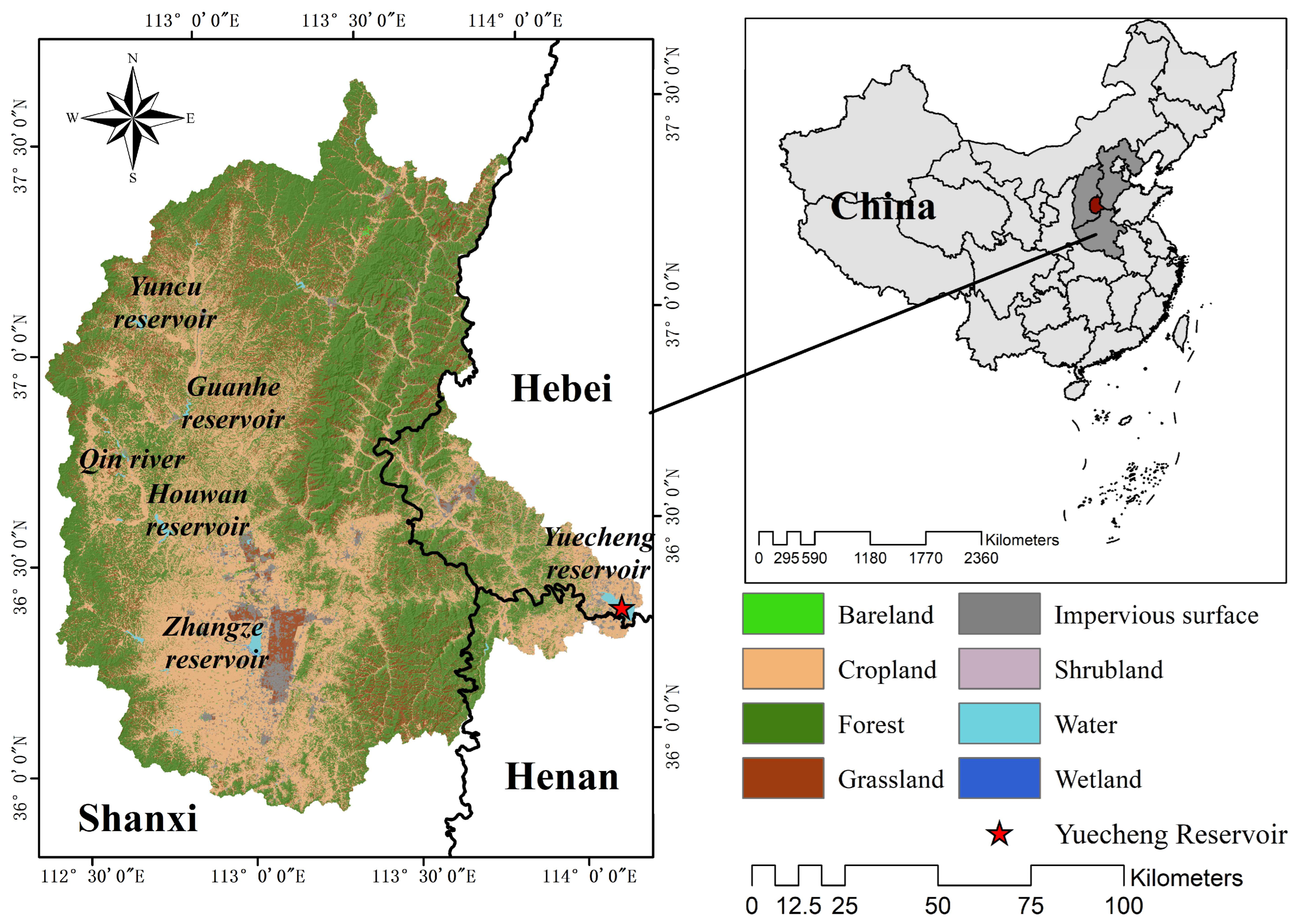
2.1. Study Area

Yuecheng Reservoir is located in Ci County, Handan City, Hebei Province, China. It is a national super-large reservoir that serves as an urban water supply; it integrates flood control, irrigation, power generation, and other functions. It is an important water source for Handan City, Hebei Province, and Anyang City, Henan Province, with a storage capacity of nearly 1.3 billion m3. The control catchment area of the Yuecheng Reservoir (i.e., the study area) is 18,072 km2 and is located at 112°26′~114°14′E and 35°52′~37°36′N. Although Yuecheng Reservoir is in Hebei Province, most of the catchment area of the Yuecheng Reservoir is in Shanxi Province, as shown in Figure 1. The Yuecheng Reservoir catchment is located in the southeast of the Loess Plateau with complex terrain and high average altitude which is above 1000 m.
The Yuecheng Reservoir catchment area is dominated by agricultural production. The main crop types include maize, wheat, millet, soybean, and sorghum; maize is the main crop in summer and wheat is the main crop in winter. The multiple cropping index in the study area usually fluctuates between 0 and 2; the crop rotation mode is mostly winter wheat/summer maize. The terrain of the study area is complex, and the central part is penetrated by the main vein of Taihang Mountain from north to south. The soil type of the study area is mainly loam, with a small amount of sand. The study area is divided into east and west areas, each with their own typical characteristics. The eastern region comprises mostly rocky mountainous areas with high mountains and deep valleys. With the warm and humid air flow from the southeast, heavy rains are easily produced under the action of surface lifting. Additionally, the underlying surface has good production and confluence conditions, which leads to large floods in this area; thus, NSP also flows into the major rivers during periods of flooding, causing water pollution. The western region is surrounded by mountains, the central part is a basin, and the southern part contains limestone areas with developed fissures and serious leakage. Other marginal areas in the western region are rock mountainous areas with steep terrain. These areas experience extensive water and soil loss, and they are the main sources of sediment runoff in the Yuecheng Reservoir catchment area [51]. The complex cultivated land situation, coupled with the influences of the terrain and climate, has created NSP that has considerably influenced the water quality of the Yuecheng Reservoir.

2.2. Data and Preprocessing
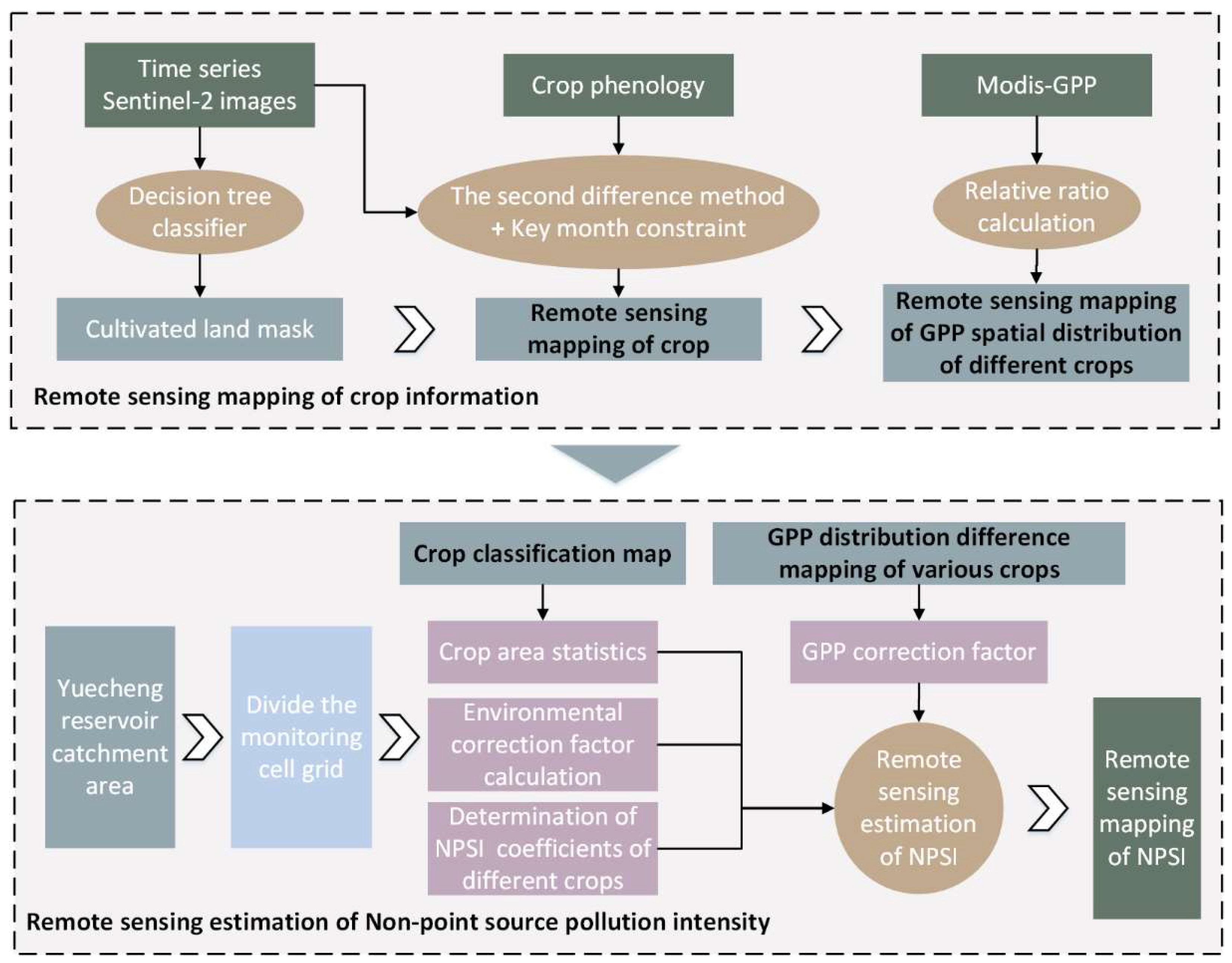
The basic data of Yuecheng Reservoir mainly included geographic data and statistical data. Specifically, the geographic data comprised remote sensing multispectral images, digital elevation model (DEM) data, and precipitation and soil type data; the statistical data included fertilizer application, crop area, phenology, and yield information (Table 1).
After considering the factors of space, time, and spectral resolution we chose Sentinel-2 images for use as the remote sensing images in this experiment. The Sentinel-2 satellite carries a multispectral imager, which can cover 13 spectral bands with a width of 290 km. The spatial resolutions of different spectral bands are 10 m, 20 m, and 60 m, respectively. Sentinel-2A and Sentinel-2B satellites complement each other, and the revisit cycle can reach 5 days. We chose appropriate months for cultivated land and crop type mapping according to crop phenology. Specifically, high-quality Sentinel-2 images with few or no clouds were selected during the period from January to December 2019. The downloaded Level 2A Sentinel-2 data were orthophoto-, geometric precision-, and atmosphere-corrected; thus, pre-processing only comprised splicing and clipping. Because we could not find high-quality images with few or no clouds in the region in February 2019, we interpolated images from adjacent months, namely January and March 2019, to obtain the February image.
DEM data and soil type data required pre-processing that included splicing, clipping, and resampling to a resolution of 10 m. GPP data were based on the MOD17A2 dataset provided by the National Aeronautics and Space Administration (NASA), which is an 8-day synthetic product of GPP with a spatial resolution of 500 m. These data were preprocessed by batch clipping and resampling.
Tropical rainfall measuring mission (TRMM) precipitation data were based on the TRMM 3B42 daily dataset provided by NASA, which has a spatial resolution of 0.25°. To ensure that the precipitation distribution was consistent with actual observations, Kriging interpolation was carried out by using the central point position of each pixel of TRMM data as the interpolation point.
The statistical data of chemical fertilizer were acquired by searching the statistical yearbook. The data were then spatialized according to county boundaries.

3. Methodology

The flowchart of this paper is shown in Figure 2. This study consists of two main parts: the remote sensing mapping of crop information using the phenology–GPP method and the remote sensing estimation of agricultural NSP. In Section 3.1, based on Sentinel-2 images and MODIS-GPP data acquired in 2019, we extract cultivated land and crop types. Then we simulate the differences in spatial distributions of crop growth in the Yuecheng Reservoir catchment area to estimate agricultural NSP. In Section 3.2, we introduce the calculation formula of NSP intensity for refining crop impact. In Section 3.3, we describe the methods for the verification of crop classification and crop growth spatial difference simulation.

3.1. Phenology–GPP Method for Crop Classification

3.1.1. Remote Sensing Mapping of Cultivated Land

A cultivated land map in the study area is required to estimate NSP intensity. The accuracy and available years of existing land use products are limited. For cultivated land, the phenomenon of abandonment often occurs, and it happens randomly according to the will of farmers. Therefore, it is necessary to obtain the annual high-precision cultivated land map. We went to the study area and collected data. We found that the main land uses in the study area include water, impervious surface, bare land, cultivated land, forest land, shrubland, and grassland. To obtain the cultivated land map, we needed to distinguish it from other land uses. We collected 30 field samples of each land use (each sample contains 3 × 3 pixels) for the average spectral test, as shown in Figure 3. Firstly, we divided land uses into vegetation and non-vegetation and compared the effects of different vegetation indices.
In practical application, NDVI and EVI are widely regarded as the best indexes for vegetation identification. We compared them. As shown in Figure 4, NDVI is better than EVI in distinguishing vegetation from building land and water. We have counted the NDVI and EVI values of each land uses sample, which can also prove that NDVI is more effective in extracting vegetation in the study area, as shown in Figure 5. The study area is a semi-arid area with low FVC (fractional vegetation cover). NDVI is sensitive in low FVC area, but it is easy to saturate and is not suitable for high FVC area. EVI is often used in densely vegetated areas. In this experiment, it is clear that NDVI is more suitable.
Vegetation includes shrubland, grassland, forest land, and cultivated land. It is also necessary to separate cultivated land from other vegetation. As shown in Figure 3, the reflectance of forest in red band is generally lower than shrubland, grassland, and cultivated land. The FVC of forest and cultivated land is usually higher, while that of shrubland and grassland is usually lower. Therefore, when distinguishing forest land and cultivated land, it is necessary to use vegetation index sensitive to high FVC areas. Figure 6 shows the sensitivity of each vegetation index in different FVC. The results showed that RVI was more sensitive in high FVC areas, while NDVI was more sensitive in areas of low vegetation coverage. RVI is not only sensitive to high FVC areas but can also magnify the difference of each vegetation in red band, which is more effective in identifying forest. The spectral curves of shrubland and grassland are very similar to that of cultivated land, which cannot be distinguished by general vegetation indices. VIUPD index is more advantageous in reflecting vegetation types by the linear decomposition of the reflectance of soil, water, vegetation, and yellow leaves. As shown in Figure 9c, experiments on samples collected from cultivated land, shrub land, and grassland showed that VIUPD could effectively identify cultivated land.
We identified cultivated land using Sentinel-2 images from 2019 based on the above analysis. Zhu [52] used the method of decision tree classification to classify the land use types of the Yuecheng Reservoir catchment. To identify cultivated land, we divided the decision tree into five levels (Figure 7a) according to this method. Each level removed a class of typical features, ultimately yielding a distribution map of the cultivated land. The normalized difference water index (NDWI) was used for water identification to separate water from land. Compared with other water indices, NDWI can enhance water signals by effectively suppressing vegetation signals. Our aim was to identify cultivated land, so more attention was paid to the index’s ability to distinguish between other features and vegetation. Based on the land map, NDVI was used to separate vegetation and non-vegetation areas. Compared with other vegetation indices, NDVI is more sensitive to vegetation with low and medium FVC, so it is effective in distinguishing vegetation from non-vegetation. August is the most productive month with respect to vegetation growth in the Yuecheng Reservoir catchment area, and the NDVI value approaches its maximum for the whole year during this month, thereby enabling vegetation to be distinguished from non-vegetation. For some winter single crops, the cultivated land is in a fallow state in August and the NDVI value is small. Thus, winter single crops were missed when mapping only using the images from August. The identification of vegetation is not accurate enough, and some planting areas of winter single crops cannot be identified as vegetation. To aid in avoiding this problem, we used the maximum synthesis method [53] for the annual NDVI time series images to obtain NDVImax and set the appropriate threshold to get the vegetation distribution map. From the vegetation map, we need to identify the shrubland, grassland and forest land to get the map of cultivated land. The FVC of grassland and shrubland is lower than that of cultivated land and forest. After comparing the values of the universal pattern decomposition (VIUPD) index in a large number of vegetation samples, we found that the VIUPD could differentiate shrubland and grassland from other vegetation. To identify cultivated land from forest, the ratio vegetation index (RVI) was used. Forest and cultivated land have high FVC, and RVI is just sensitive to vegetation with high FVC. Based on large vegetation samples, RVI has the ability to separate cultivated land from forest. The thresholds of these indices are general empirical values. Finally, after the removal of other features at each level, we obtained the remote sensing mapping results of cultivated land. Table 2 lists the spectral indices used in this study.

3.1.2. Crop Classification

After obtaining the distribution map of cultivated land in the Yuecheng Reservoir catchment area, we classified the crops. According to the statistical yearbook and field investigation, the main crops in the Yuecheng Reservoir catchment area include corn, millet, and winter wheat. Corn is the main crop, constituting approximately 70% of the total crops. The multiple cropping index is between 0 and 2, and the cropping rotation is mainly winter wheat and summer corn [58]. A fraction of cultivated land in the study area is only planted with winter wheat each year. To provide a better estimate of the intensity of agricultural NSP, we divided the crops into multiple cropping, winter single crops, and summer single crops in the study area. In order to construct a crop classification method, we collected the local main crops’ phenology data from the ministry of agriculture planting industry management (http://www.zzys.moa.gov.cn/ (accessed on 11 November 2020)) and the national meteorological science center (http://data.cma.cn/ (accessed on 19 November 2021)), as shown in Table 3.
In addition, we collected some crop samples (including multiple crops, winter single crops and summer single crops) from real locations in the field. The corresponding curves of each crop samples were extracted from the time series NDVI image, and the typical curve of each crop was shown in Figure 4b. By analyzing crop phenology information and these typical NDVI curves, we constructed a crop classification method. The crop classification process is shown in Figure 7b. This method consists of two steps: first, crops were classified as either single or multiple crops; second, single crop areas were divided into summer and winter crops.
Step 1: To identify multiple crops, we first used the second difference method [59] to detect peak values of NDVI time series images for the year. The principle of the second difference method is as follows:
NDVI i = NDVI i NDVI i 1
NDVI i = { 1 , NDVI i > 0 1 , NDVI i < 0
NDVI i = NDVI i + 1 NDVI i
where NDVI is the annual NDVI value time series of each pixel position, NDVI represents the first difference value sequence of each pixel position, NDVI is the assignment of the first difference result, NDVI represents the second difference value sequence, and i (i ≤ 12) represents the ith month. The NDVI sequence at each pixel position has 12 values, the NDVI and NDVI sequences have 11 values, and the NDVI sequence has 10 values. There are only three possible values of N D V I i : −2, 0, and 2. When N D V I i is −2, the corresponding time phase point i is the crest.
Combined with the specific phenology of crops and the typical tillage methods in the Yuecheng Reservoir catchment area, the node with the peak value is used to identify the multiple crops, in accordance with local conditions. As shown in Figure 8, winter crops (mainly winter wheat) in the Yuecheng Reservoir catchment area are usually sown in October and harvested in June of the next year, while summer crops (70% corn) are commonly sown in June and harvested in October. When the crops grow, the NDVI gradually increases. When the crops begin to mature, the NDVI value decreases along with the crop chlorophyll concentration [1]. Winter crops gradually mature from April to May, while summer crops mature in August. Therefore, these time periods coincide with the peak NDVI value of crops for the year. The peak value detected by the second difference method is constrained by month. When the peak value is detected simultaneously in April (or May) and August, the corresponding pixels are identified as multiple crops.
Step 2: To distinguish summer single crops and winter single crops, we analyzed the NDVI time series images of field sampling points. The most obvious difference between summer single crops and winter single crops was that the NDVI of winter single crops gradually decreased from May to June, whereas the NDVI of summer single crops and other vegetation gradually increased. Therefore, we used the following formula to distinguish the two NDVI values:
N D V I J u n N D V I M a y < 0
where N D V I J u n and N D V I M a y represent the NDVI value of each pixel in June and May, respectively.

3.1.3. Remote Sensing Mapping of the Spatial Distribution Difference of Crop Growth

For a catchment with large area and wide coverage, there must be a significant difference in the spatial distribution of crop growth conditions (i.e., the quality of cultivated land). The absorption of fertilizer depends on crop growth. If the crops grow well, comparatively few pollutants remain in the environment, otherwise poor crop growth leads to substantial pollutant presence. MODIS-GPP data reflect the quality of cultivated land through biomass representation [51]. It is necessary to calculate the total GPP of crops during the growth period as an approximation of the growth statuses of those crops. In this experiment, if there were multiple crops, then we added the annual GPP. For winter single crops, we added the GPP from June to September, and for summer single crops, we added the GPP from October to May of the next year. Finally, we used the cultivated land quality correction coefficient ε i to reflect the spatial differences in crop growth in the catchment area, as follows:
ε i = P i x e l G P P i M e a n G P P i
where P i x e l G P P i represents the GPP value of the current pixel of class i cultivated land and M e a n G P P i represents the mean GPP of class i cultivated land within the catchment area.

3.2. Pollution Source Intensity Calculation Method

After obtaining the crop distribution map using 10-m-resolution Sentinel-2 images, we calculated NSP intensity. To facilitate the zoning management of farmland, the Yuecheng Reservoir catchment area was divided into 1 km × 1 km grids to calculate NSP intensity. First, we calculated the areas of all kinds of cultivated land using the following formula:
A i = n = 1 q n × p 2
where A i is the planting area of cultivated land type i in the grid, n is the number of pixels, p is the spatial resolution of the pixel (10 m in this study), and q is the number of pixels identified as cultivated land type i.
To calculate the spatial distribution characteristics of the emission potential of total nitrogen (TN) and total phosphorus (TP) in farmland, we improved the calculation formula of farmland NSP intensity proposed by Zheng et al. [1] and added the farmland quality correction factor. The specific calculation method is as follows:
Q TN = i n A i × TN i × 1 / ε i × M
Q TP = i n A i × TP i × 1 / ε i × M
M = S × A × F × P
where Q TN and Q TP are the TN and TP emissions from agricultural production, respectively; i is the type of cultivated land and n is the total number of farmland types, including multiple crops, winter single crops, and summer single crops. TN i   and   TP i are the NSP intensity coefficients of pollutants TN and TP of the ith crop, respectively; the specific values are listed in Table 4. ε i is the cultivated land quality correction coefficient of the ith crop, which can be obtained using Equation (5). M is the total environmental correction coefficient; S, A, F, and P are the correction coefficients for slope, soil type, fertilizer amount, and annual precipitation, respectively (Table 5). The above correction coefficients TN i ,   TP i , and M are determined in accordance with the requirements of “The Technical Guide for National Water Environmental Capacity Verification” [60] issued by the State Environmental Protection Administration of China. The “National Technical Guide for the Verification of Water Environment Capacity” provides the source intensity coefficient of winter wheat, which is commonly used to represent all crop types in traditional methods. We determined the source intensity coefficients of multiple crops and summer single crops by consulting the literature [61,62,63] and combining factors, such as the amount of fertilizer applied and the amount of crop absorption. In our study area, we focused on three common crop types. In practical application, more cultivation modes (e.g., more than single-year crops) would require the determination of source intensity coefficients from empirical values or field experiments [60].
For the correction of crop growth factor, the “National Technical Guide for Verification of Water Environment Capacity” provides the environmental conditions of standard farmland when determining the source intensity coefficient. It clearly indicates the approximate range of each correction coefficient for specific environmental conditions. On this basis, we stratified the correction coefficient more carefully to facilitate accurate source intensity calculation. The crop growth correction is an additional step in the existing process. Because we were focused on calculating the NSP source intensity of a large-scale catchment, spatial differences in crop growth could not be ignored. For different crops, crop quality was corrected by GPP.

3.3. Crop Information Verification Method

To verify the accuracy of remote sensing mapping of crops in the Yuecheng Reservoir catchment area, we collected field samples of multiple crops, winter single crops, and summer single crops. Next, we superimposed these samples on high-resolution Google Earth images for artificial digitization. The overall size of the samples was consistent with the size of the field cultivated land. To ensure verification method objectivity, a mixture matrix was used to calculate the classification accuracy. User accuracy, producer accuracy, overall accuracy, and the kappa coefficient were used to quantify the accuracy of the crop classification results. User accuracy represents the probability that the classifier recognizes a specific type of ground object, and its corresponding real type is also this type of ground object. Producer accuracy represents the probability that the type is a feature and is recognized as that feature by the classifier. Overall accuracy represents the proportion of all correctly classified samples in the total number of samples. The values of these three quantitative indicators are between 0 and 1, where values closer to 1 indicate higher classification accuracy. The kappa coefficient was used to evaluate whether the classification results of the classifier were consistent with the actual observations, and its value is between −1 and 1, where values closer to 1 indicate higher classification model accuracy.
To verify the remote sensing mapping of the spatial distribution difference of crop growth in the Yuecheng Reservoir catchment area, we divided the study area into its constituent counties, then fitted the yield per unit area of various crops in each county’s statistical yearbook with the county’s mean cultivated land quality correction coefficient. The goodness of fit R 2 was used to measure the degree of fitting. The value range of R 2 is between 0 and 1, where values closer to 1 indicate better fitting effect.

4. Results

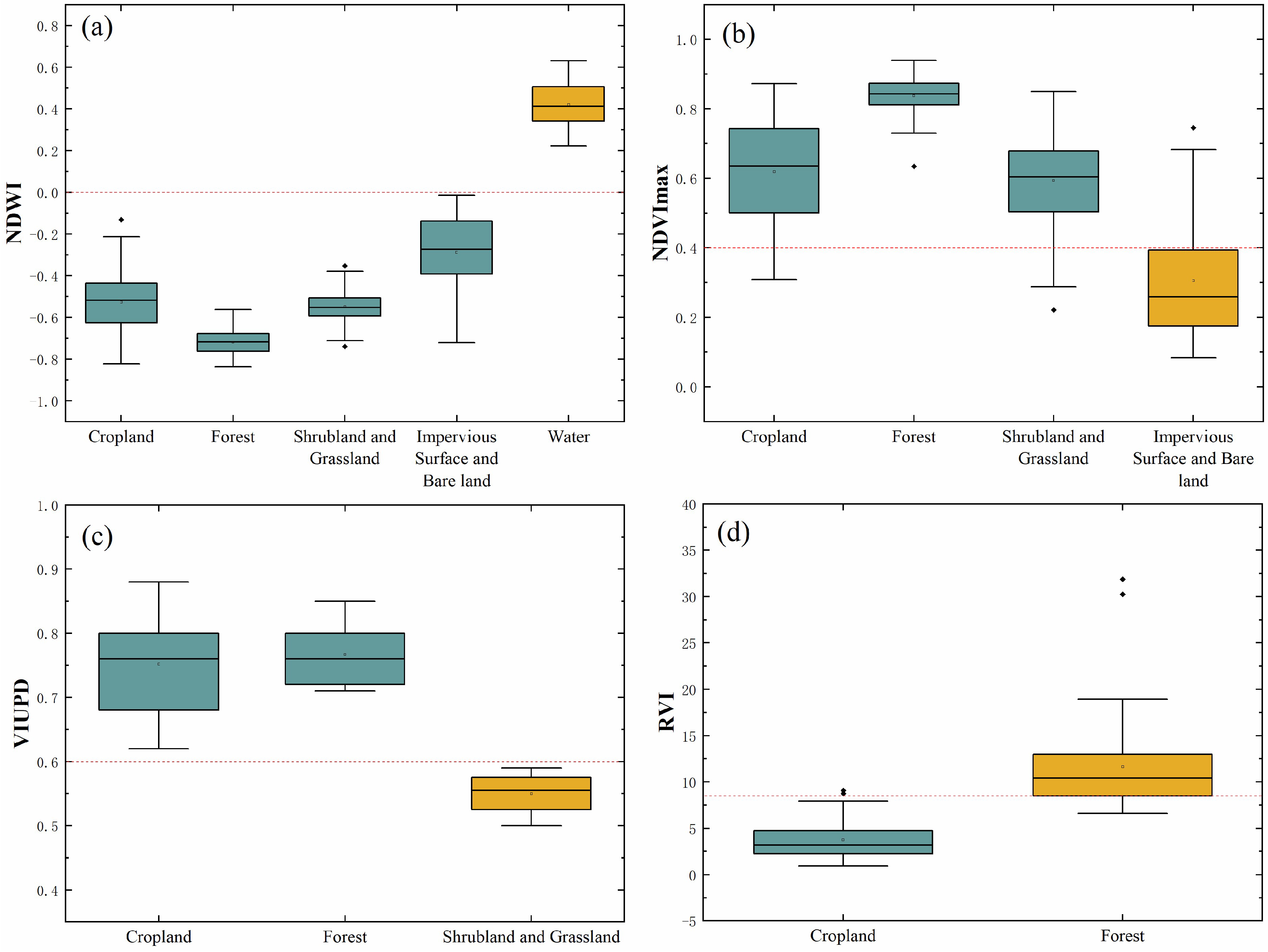
4.1. Thresholds Analysis in Cultivated Land Mapping

We used the decision tree method to identify cultivated land from the Yuecheng Reservoir catchment area. By fully utilizing the advantages of each index, each level of the decision tree removes a particular type of ground object through index calculations. Finally, the distribution of cultivated land is obtained at the last level of the decision tree. First, NDWI was used for water identification. Vegetation was separated from water, impervious surface, and bare land by the NDVI. In this work, the challenge lies in distinguishing cultivated land from other vegetation. Therefore, we analyzed the differences between cultivated land and other vegetation under different vegetation indices. The results showed that the VIUPD value of shrubland and grassland was significantly different from the VIUPD values of forest land and cultivated land. The RVI separated forest land and cultivated area. To determine the thresholds, we selected 50 samples of each type of ground objects and evaluated the calculation results of their indices. Figure 9 shows good discrimination among the various ground objects under specific indices.
Figure 9. Box diagram of remote sensing index of typical surface features. (a) NDWI can distinguish water from other surface features when the threshold is 0. (b) NDVI synthesized by the annual maximum value can distinguish impervious surface and bare land from vegetation when the threshold is 0.4. (c) VIUPD index (mainly including cultivated land, forest land, shrubland, and grassland) can distinguish shrubland and grassland from the other two types of land when the threshold is 0.6. (d) RVI statistical value of cultivated land and forest land samples demonstrates good separation when the threshold is 8.5. Finally, the distribution map of cultivated land is obtained (the yellow boxes show the indices values of identified ground features, and the green boxes show the indices values of other land use types).
Remotesensing 14 02833 g009

4.2. Crop Classification in the Yuecheng Reservoir Catchment Area

By analyzing the growth curves of the main crops in the Yuecheng Reservoir catchment area, combined with data from the Sentinel-2 images for the year, we first identified the distribution of multiple crops. To facilitate the calculation of NSP intensity, we separated single crops into winter single crops and summer single crops. Most of the crops in the catchment area were summer single crops, and 70% of the crops in the area were summer maize. Because of regulatory policies in each county, multiple crops and winter single crops showed aggregation distributions. Combined with Google Earth high-resolution remote sensing images, we verified the accuracy of crop classification results in the Yuecheng Reservoir catchment area by analyzing 50 samples of multiple crops, summer single crops, winter single crops, and other surface feature types (including water, impervious surface, bare land, and other vegetation). The results are shown in Table 6. The decision tree and crop phenology showed good precision. The producer accuracy and user accuracy of each type of feature exceeded 70%. The overall accuracy and kappa coefficient indicated that the crop classification results were highly consistent with actual observations. The spatial distribution of crops in the Yuecheng Reservoir catchment area is shown in Figure 10.

4.3. Remote Sensing Mapping of Spatial Distribution Difference of Crop Growth in the Yuecheng Reservoir Catchment Area

The Yuecheng Reservoir catchment area covers 18,072 km2 and spans three provinces, including 18 counties. The spatial distribution of crop growth differs from this catchment area boundary. To accurately estimate the NSP intensity, it is necessary to simulate the crop growth in the study area (i.e., spatial difference in cultivated land quality) to correct for differences in NSP intensity. To verify the cultivated land quality simulation results, the study area was divided into counties and fitted according to the output per unit area of various crops in the statistical yearbooks of each county, as well as the correction coefficient of mean cultivated land quality in the county. R 2 was >0.7, indicating that these values had good consistency. The spatial distribution of cultivated land quality is shown in Figure 11.

4.4. Estimation of NSP Intensity in the Yuecheng Reservoir Catchment Area

The NSP intensity was estimated for the cultivated land area in the Yuecheng Reservoir catchment area (Figure 12a). The results indicated a concentration area of high source intensity of farmland NSP southwest of the Yuecheng Reservoir catchment area. The NSP intensity decreased gradually to the north and decreased sharply to the east. The overall trend corresponded to the topographic relief, cultivated land area of each county, crop yield, crop environmental conditions, and other factors in the region. The main vein of the Taihang Mountains runs through the middle of the Yuecheng Reservoir catchment area from north to south, and most of the area to the east of the Taihang Mountains is rocky with high mountains and deep valleys, exposed rocks, and little cultivated land. This leads to decreased farmland NSP from the middle to the East. The main factor affecting the gradual reduction of the NSP intensity from south to north in the central and western regions is the crop growth environment. Among these regions, the Changzhi, Lucheng, and Xiangyuan counties are basins with flat terrain and abundant rainfall, which are suitable for crop growth, and multiple crops are mostly concentrated in this area. In addition, the statistical yearbook data indicate that the cultivated land area and fertilization are higher in these counties than in other counties, which makes these counties more likely to serve as sources of pollution.

5. Discussion

5.1. Different Contributions of Crops to NSP Intensity

There are great differences in nutrient requirements, actual fertilization, fertilizer utilization rate, and fertilization node for different crops [64]. Taking winter wheat and summer maize in the study area as an example, winter wheat needs more nitrogen than summer maize but less phosphorus than summer maize [65,66]. This directly affects the actual fertilization. To make crops grow better, farmers use different fertilization schemes for different crops. Fertilization schemes differ not only in the proportion of nutrients but also in the time nodes of fertilization. For winter wheat, it is necessary to apply starter fertilizer in October of each year and topdressing in the rejuvenation stage, jointing stage, and early filling stage. These growth stages of winter wheat in this study area are, respectively, in March, April, and May of the following year. For summer maize, it is necessary to apply starter fertilizer in June every year and topdressing in the great bell mouth stage and tasseling stage. The two growth stages of summer maize in this study area are July and August, respectively. The study area is in the same period of rain and heat. It is cold and rainy in winter but warm and rainy in summer. In October, March, and April, when winter wheat was fertilized, precipitation was less, while during the summer maize fertilization, precipitation was more. This indicates that not only the fertilization, crop fertilizer absorption rate, and other factors affect the generation of NSP intensity but also that the precipitation at the time of fertilization affects the loss of pollutants. If multiple cropping exists in the study area, crops are planted all year round and the frequency of fertilization increases significantly, which also affects the generation of NSP intensity [64].
The difference of NSP intensity caused by different crop types is only one aspect. For a large watershed, even for the same crop type, their growth situation is different due to their different growth environments [67]. Under certain conditions, the more dry matter fixed by photosynthesis, the better the growth of crops [51,68], the better the absorption of fertilizer, and the fewer pollutants discharged into the environment. This is also an important factor in the estimation of NSP intensity.
Different types of crops, different planting patterns, and different growth potential have different contributions to NSP. In addition, soil type, precipitation, slope, fertilization differences between different farmers, and other factors also affect the estimation of NSP intensity. Therefore, the mapping of NSP intensity has always been a difficult problem. Zheng et al. [1] proposed a traditional method for NSP intensity estimation. It uses a unified source intensity coefficient to estimate NSP intensity generated by farmland, without considering the effects of crop types or growth on it. The results of the NSP intensity estimation are shown in Figure 12b. Compared with the method in this paper, without fine crop classification and growth information, it cannot reflect the real NSP intensity.
Compared with the NSP intensity estimated using the proposed method shown in Figure 13, the estimations were consistent with the overall trend. But there were considerable differences in the specific estimated quantities of each unit. This is because the method presented in this paper considers crop types and growth. For example, more fertilizer is applied in multiple cropping areas than in single cropping areas, so more NSP is generated. Therefore, the maximum NSP intensity throughout the study area estimated by the proposed method was more than it obtained by the traditional method. Figure 13 shows differences in the estimation of local NSP intensity. It is obvious that there are various types of crops in each 1 km × 1 km grid. Different types of crops lead to different contributions to NSP intensity. All crop types cannot be considered as one category. In addition, when traditional methods are used to estimate TN and TP, the spatial distribution trends of the estimation results will be identical because the NSP intensity coefficients are fixed and interrelated values. Importantly, compared with single crops, the NSP intensity coefficients of TN and TP for multiple crops do not increase by the same magnitude [63]. Therefore, the spatial distribution trends of these values are slightly different, and these differences are not well represented by traditional methods. In general, crop types, growth status, and growth conditions cannot be ignored in NSP intensity estimation and mapping. The method in this paper is a reasonable modification to the traditional method.

5.2. The Importance of Remote Sensing in Large-Scale NSP Intensity Mapping

Because of the randomness, lag, and fuzziness of NSP, there are many problems in its mapping and quantification. Considering that the geographical databases of many countries and regions worldwide are imperfect and cannot meet the parameter requirements of the NSP estimation model, they cannot be applied to large-scale NSP intensity estimation [69]. Remote sensing technology can provide high precision geographic data for NSP intensity mapping. With the development of precision agriculture, cultivated land management is becoming more information-intensive, and the cultivation mode is becoming more complex [70]. To maximize the income of cultivated land, multiple cropping generally exists in countries and regions with less cultivated land per capita, which complicates the calculation of NSP intensity. Particularly among large-scale areas, the methods of cultivated land management differ substantially. The field measurement of NSP intensity is both time- and labor-intensive. With the characteristics of high speed, timeliness, and reliability, remote sensing technology has great advantages in large-scale target identification and mapping. The use of remote sensing technology can realize the fine classification and information mining of crops [71]. Remote sensing makes it possible to accurately estimate NSP intensity in larger scale areas.

5.2.1. Crop Spatial Information Mapping in Large-Scale Area from Remote Sensing

Remote sensing technology has made great achievements in large-scale crop information recognition. NSP intensity estimation depends on large-scale remote sensing data. In all remote sensing models, the index method is widely used in ground object identification because the approach is simple, with fast processing speeds and high accuracy [72]. We identified cultivated land by constructing various indices into decision tree. We determined the segmentation threshold of each index with a large number of samples, thus making a reliable distribution map of cultivated land. This method can be extended to other areas, because the study area in this paper covers the vast majority of ground objects. The vegetation index thresholds should be determined based on local conditions. We used the second difference method [59] to detect the peak of NDVI time series images to map the distribution of multiple cropping areas. Before peak detection, it was necessary to have a preliminary understanding of the crops in the study area, as well as a general understanding of the area’s crop types and cultivation modes. For example, maize is the main crop in our study area, and two cultivation modes are used: multiple cropping and single cropping. Winter crops grow best in April and May, while summer crops grow best in August. Therefore, using these critical time nodes to constrain the time when the peak occurs can reduce the misclassification of multiple crops. When this method applied to other regions, it is only necessary to obtain the phenology of general crops and multiple crops in the research area, then obtain the key phenological nodes of vigorous crop growth to identify multiple crops. As shown in Table 6, the classification results of this method are generally reliable. For the study of cultivated land quality, the NDVI [73], Enhanced Vegetation Index [74], and GPP [51] are used in remote sensing mapping of crop growth. Among them, the GPP reflects the total amount or fixed total inorganic energy that plants synthesize into organic matter per unit time and per unit area, which is more suitable for crop growth monitoring. This experiment focuses on the remote sensing the identification of crop types, multiple cropping, and growth information and uses them as parameters to modify the existing NSP intensity model. The existing remote sensing technology is mature enough to obtain larger-scale geographic data, and this paper only takes the catchment area of the Yuecheng Reservoir as a case study. The method mentioned in this paper can be applied to larger scale regions.

5.2.2. Potential for Large-Scale NSP Intensity Estimation from Remote Sensing

At present, the research on NSP has been limited to the watershed. NSP mapping for a larger scale has been unable to break through [75]. The main reasons for this are as follows: First, the NSP itself. NSP has the characteristics of fuzziness, lag, randomness, universality, and latency. When estimating on a large scale, these characteristics make the estimation more difficult. Second, the problem of NSP model. In the existing NSP models, both physical models and empirical models have their own disadvantages, which makes large-scale application very difficult. The main problem lies in the acquisition of parameters. If we want to obtain more accurate estimates of NSP intensity, we need more and more accurate field data. However, the measurement of these data often takes a lot of time, energy, and money [76]. Remote sensing can solve this problem and obtain ground inversion and classification data in a short time. In addition, the NSP intensity estimation combined with remote sensing can overcome the problem of the low efficiency of the distributed model and the low accuracy of lumped model. Taking rich large-scale remote sensing data as input parameters can refine the method of over averaging in the lumped model. It not only makes the results more accurate but also avoids the problem of low calculation efficiency caused by the need to partition the large-scale region in the physical model. Secondly, the temporal and spatial characteristics of remote sensing can also provide long-term and time-effective data sources, which makes it possible to study the multi-year variation and lag of NSP [77].

5.3. Management Strategies

Zheng et al. [1] developed a NSP intensity calculation method in accordance with the requirements in the “National Technical Guide for Verification of Water Environmental Capacity”, issued by the State Environmental Protection Administration of China, which has been widely used in the estimation of NSP in river basins [1,29,31,32]. Now this method is quite developed. In this study, we have improved the method in principle, so that it better reflects the crop types and crop growing condition. We modified the coefficients according to crop types, environment, and crop growth quality. The method is thus applicable for NSP intensity calculations in different environments. This study improves the existing methods combined with remote sensing technology and takes the catchment area of the Yuecheng Reservoir as an example to estimate and map the NSP intensity on a large scale. This fully proves the great potential of using remote sensing technology in large-scale NSP estimation and mapping. In the future, we can also consider using more sufficient geographic data for larger-scale NSP estimation, so as to make the method more perfect and the results more reliable.
Most NSP models only focus on the actual amount of non-point source pollutants in rivers but ignore the source and migration of pollution. This is not very useful for NSP control and management. NSP intensity mapping can reflect the capacity of land to generate pollutants. For cultivated land especially, crop types, planting mode, fertilization, and growth environment affect its contribution to NSP. NSP formation is a complex and ambiguous process. To efficiently manage NSP, various management measures and technologies have been developed. Yang et al. proposed a “4R” strategy to more systematically and comprehensively manage NSP, which greatly improves control in agricultural applications [78]. The model is mainly composed of four steps: source reduction, process retention, nutrient reuse, and ecological restoration. Among these steps, source reduction is the key measure for mitigation of agricultural NSP [33]. This paper solved the problem of NSP source monitoring, which is a very key part of the “4R” strategy. NSP intensity map can make source control more targeted and strengthen management in places with high source intensity. Local governments can guide the planting mode of crops and the layout of farmland in conjunction with water quality. Poor agricultural management leads to soil erosion, as well as greater nitrogen and phosphorus losses in surface runoff, thus resulting in the formation of a large area of farmland NSP in the surrounding catchment [79]. The topic discussed in this paper is to extract crop information through remote sensing technology and then estimate the NSP intensity based on the contribution of different crops, which is a forward process. For management, it needs to be considered conversely. For the heavily polluted areas identified in the NSP intensity map, it is necessary to pay attention to the adjustment of crop planting mode and fertilization strategy to minimize the emission of pollutants. In addition to source control, the application of remote sensing in pollutant interception also has great potential. It can help design pollutant buffers, riparian, and so on [80]. It also plays a role in all aspects of NSP management.
From the perspective of precision agriculture management, farmland grid management is a convenient and efficient management method which can break the constraints of administrative units and improve the efficiency of information retrieval/renewal [81,82]. In this study, the source intensity was estimated by grid division, which improves the efficiency of cultivated land retrieval. In farmland management, the application amount of chemical fertilizer can be controlled hierarchically according to grids with different NPS intensity. In a grid with considerable source intensity, the application of chemical fertilizer would be reduced accordingly. In contrast, for grids with low NPS intensity, the amount of chemical fertilizer can be reduced or even not reduced. In this manner, farmland NSP can be controlled while maximizing crop yield. This facilitates the control of NSP and the management of precision digital agriculture.

6. Conclusions

In this study, we proposed a phenology–GPP method to classify crops for the estimation of source intensity in farmland NSP sensitive areas, thereby solving the problem of differences in NSP intensity distributions caused by different crop types, multiple cropping, and crop growth. Sentinel-2 high-resolution remote sensing images were used to extract the temporal and spatial features of crops. First, the decision tree classification method was used to identify the cultivated land in the Yuecheng Reservoir catchment area. Then, the distributions of multiple crops, winter single crops, and summer single crops were identified using the second difference method combined with month constraints. The overall accuracy of crop mapping is 85% and the Kappa coefficient is 0.8. Because crop growth is not considered in traditional models, MODIS-GPP data were used to simulate crop growth and modify the parameters of the existing model. Finally, the spatial distribution of NSP intensity in the Yuecheng Reservoir catchment area was calculated. Compared with the traditional model, the improved model highlights the differences in the spatial distributions of TN and TP, and it also provides a source intensity estimation result that is closer to actual values because it ensures the precise simulation of farmland status. This provides a reliable decision-making basis for controlling NSP and managing farmland, and it is conducive to more targeted and efficient management and mitigation strategies.

Author Contributions

Conceptualization, M.L., T.W. and S.W.; Data curation, M.L.; Formal analysis, M.L.; Funding acquisition, T.W. and S.W.; Investigation, T.W.; Methodology, M.L.; Project administration, M.L.; Resources, T.W.; Software, M.L.; Supervision, T.W., S.W., S.S. and Y.Z.; Validation, M.L.; Visualization, M.L.; Writing—original draft, M.L.; Writing—review and editing, M.L., T.W. and S.W. All authors have read and agreed to the published version of the manuscript.

Funding

Research grants from the Specially-Appointed Professor program of Jiangsu province and National Natural Science Foundation of China: 42141007; Inner Mongolia Autonomous Region Science and Technology Achievement Transformation Special Fund Project: 2021CG0045.

Conflicts of Interest

The authors declare no conflict of interest.

References

  1. Zheng, D.; Wang, L.; Zeng, H.; Yang, S.; Zhang, C.; Liu, Y. A simulation of non-point source (NPS) pollution loads in Songtao reservoir catchment. Acta Sci. Circumst. 2009, 29, 1311–1320. [Google Scholar]
  2. Ding, M.; Chen, Q.; Xin, L.; Li, L.; Li, X. Spatial and temporal variations of multiple cropping index in China based on SPOT-NDVI during 1999–2013. Acta Geogr. Sin. 2015, 70, 1080–1090. [Google Scholar]
  3. Song, L. Study on Nutrients Output Change Law from Non-Point Source in Xiangxi Basin of the Three Gorges Reservoir. Ph.D. Thesis, Wuhan University, Wuhan, China, 2011. [Google Scholar]
  4. Cai, Y.; Wang, R.; Wang, L.; Liu, H.; Yang, D.; Tan, B. Effects of nitrogen amount and fertilization patterns on crop yield and nitrogen use efficiency on the North China Plain. J. Agric. Resour. Environ. 2020, 37, 503–510. [Google Scholar]
  5. Liu, Z.; Yang, P.; Wu, W.; Li, Z.; You, L. Spatio-temporal changes in Chinese crop patterns over the past three decades. Acta Geogr. Sin. 2016, 71, 840–851. [Google Scholar]
  6. Zhou, H.; Gao, C. Identifying critical source areas for non-point phosphorus loss in Chaohu watershed. Environ. Sci. 2008, 10, 2696–2702. [Google Scholar]
  7. Tu, H.; Hou, Y.; Chen, W. Simulation of non-point source pollution in Weizigou watershed with AnnAGNPS model. J. Agro-Environ. Sci. 2017, 36, 1345–1352. [Google Scholar]
  8. Tong, X.; Hu, B.; Xu, W.; Liu, J.; Zhang, P. The estimation of the load of non-point source nitrogen and phosphorus based on observation experiments and export coefficient method in Three Gorges Reservoir Area. In IOP Conference Series: Earth and Environmental Science; IOP Publishing: Bristol, UK, 2017; p. 012181. [Google Scholar]
  9. Cheng, X.; Chen, L.; Sun, R.; Jing, Y. An improved export coefficient model to estimate non-point source phosphorus pollution risks under complex precipitation and terrain conditions. Environ. Sci. Pollut. Res. 2018, 25, 20946–20955. [Google Scholar] [CrossRef]
  10. Xing, L.; Zuo, J.; Liu, F.; Zhang, X.; Cao, Q. Simulation of agricultural non-point source pollution in Xichuan by using SWAT model. In IOP Conference Series: Earth and Environmental Science; IOP Publishing: Bristol, UK, 2018; p. 012167. [Google Scholar]
  11. Ogwo, V. Streamflow and sediment yield prediction using AnnAGNPS model in upper ebonyi river watershed, South-eastern Nigeria. Agric. Eng. Int. CIGR J. 2019, 20, 50–62. [Google Scholar]
  12. Wang, W.; Chen, L.; Shen, Z. Dynamic export coefficient model for evaluating the effects of environmental changes on non-point source pollution. Sci. Total Environ. 2020, 747, 141164. [Google Scholar] [CrossRef]
  13. Hu, D.; Li, Y.; Li, L.; Zhang, C. Reduction scenarios of non-point source pollution in Xianyang-Xi’an section of Weihe River Basin based on SWAT. J. Northwest A&F Univ. 2020, 48, 127–145. [Google Scholar]
  14. Zhang, T.; Yang, Y.; Ni, J.; Xie, D. Best management practices for agricultural non-point source pollution in a small watershed based on the Ann AGNPS model. Soil Use Manag. 2020, 36, 45–57. [Google Scholar] [CrossRef]
  15. Feng, M.; Shen, Z. Assessment of the Impacts of Land Use Change on Non-Point Source Loading under Future Climate Scenarios Using the SWAT Model. Water 2021, 13, 874. [Google Scholar] [CrossRef]
  16. Buczko, U.; Kuchenbuch, R.O. Environmental indicators to assess the risk of diffuse nitrogen losses from agriculture. Environ. Manag. 2010, 45, 1201–1222. [Google Scholar] [CrossRef]
  17. Delgado, J.A.; Shaffer, M.; Hu, C.; Lavado, R.S.; Wong, J.C.; Joosse, P.; Li, X.; Rimski-Korsakov, H.; Follett, R.; Colon, W. A decade of change in nutrient management: A new nitrogen index. J. Soil Water Conserv. 2006, 61, 62A–71A. [Google Scholar]
  18. Drewry, J.; Newham, L.; Greene, R. Index models to evaluate the risk of phosphorus and nitrogen loss at catchment scales. J. Environ. Manag. 2011, 92, 639–649. [Google Scholar] [CrossRef] [PubMed]
  19. Frink, C.R. Estimating nutrient exports to estuaries. J. Environ. Qual. 1991, 20, 717–724. [Google Scholar] [CrossRef]
  20. Heathwaite, L.; Sharpley, A.; Gburek, W. A conceptual approach for integrating phosphorus and nitrogen management at watershed scales. J. Environ. Qual. 2000, 29, 158–166. [Google Scholar] [CrossRef]
  21. Jansons, V.; Busmanis, P.; Dzalbe, I.; Kirsteina, D. Catchment and drainage field nitrogen balances and nitrogen loss in three agriculturally influenced Latvian watersheds. Eur. J. Agron. 2003, 20, 173–179. [Google Scholar] [CrossRef]
  22. Johnes, P.J. Evaluation and management of the impact of land use change on the nitrogen and phosphorus load delivered to surface waters: The export coefficient modelling approach. J. Hydrol. 1996, 183, 323–349. [Google Scholar] [CrossRef]
  23. Lemunyon, J.L.; Gilbert, R.G. The concept and need for a phosphorus assessment tool. J. Prod. Agric. 1993, 6, 483–486. [Google Scholar] [CrossRef]
  24. Sharpley, A.N.; Weld, J.L.; Beegle, D.B.; Kleinman, P.J.; Gburek, W.; Moore, P.; Mullins, G. Development of phosphorus indices for nutrient management planning strategies in the United States. J. Soil Water Conserv. 2003, 58, 137–152. [Google Scholar]
  25. Arnold, J. SWAT—Soil and Water Assessment Tool; FAO: Roma, Italy, 1994. [Google Scholar]
  26. Bosch, D.; Theurer, F.; Bingner, R.; Felton, G.; Chaubey, I. Evaluation of the AnnAGNPS water quality model. In Agricultural Non-Point Source Water Quality Models: Their Use and Application, Proceeding of the Water Resources Engineering'98, Memphis, TN, USA, 3–7 August 1998; ASCE: Reston, VA, USA, 1998; pp. 45–54. [Google Scholar]
  27. Young, R.; Onstad, C.; Bosch, D.; Anderson, W. AGNPS: A nonpoint-source pollution model for evaluating agricultural watersheds. J. Soil Water Conserv. 1989, 44, 168–173. [Google Scholar]
  28. Hao, F.; Yang, S.; Cheng, H.; Bu, Q.; Zheng, L. A method for estimation of non-point source pollution load in the large-scale basins of China. Acta Sci. Circumst. 2006, 26, 375–383. [Google Scholar]
  29. Feng, A.; Wang, X.; Xu, Y.; Huang, L.; Wu, C.; Wang, C.; Wang, H. Assessment of potential risk of diffuse pollution in Haihe river basin based using DPeRS model. Environ. Sci. 2020, 41, 4555–4563. [Google Scholar]
  30. Cheng, H.; Yue, Y.; Yang, S.; Hao, F.; Yang, Z. An estimation and evluation of non-point source (NPS) pollution in the Yellow River Basin. Acta Sci. Circumst. 2006, 26, 384–391. [Google Scholar]
  31. Feng, A.; Wu, C.; Wang, X.; Wang, H.; Zhou, Y.; Zhao, Q. Spatial character analysis on nitrogen and phosphorus diffuse pollution in Haihe River basin by remote sensing. China Environ. Sci. 2019, 39, 2999–3008. [Google Scholar]
  32. Wang, X.; Wu, C.; Feng, A.; Ma, Y.; Wang, X.; Chen, M. Application of DPeRS model on estimation of non-point source pollution load of ammonia nitrogen and chemical oxygen demand in Chao Lake basin. Acta Sci. Circumst. 2015, 35, 2883–2891. [Google Scholar]
  33. Xue, L.; Hou, P.; Zhang, Z.; Shen, M.; Liu, F.; Yang, L. Application of systematic strategy for agricultural non-point source pollution control in Yangtze River basin, China. Agric. Ecosyst. Environ. 2020, 304, 107148. [Google Scholar] [CrossRef]
  34. Zhao, Y. Principles and Methods of Remote Sensing Application Analysis; Science Press: Beijing, China, 2013; ISBN 978-703-036-908-6. [Google Scholar]
  35. Yang, Y. Remote Sensing-Based Winter Wheat Identification Considering Temporal-Spectral Intra-Class Difference Characteristics of Vegetation Index. Ph.D. Thesis, Nanjing University, Nanjing, China, 2019. [Google Scholar]
  36. Panigrahy, S.; Sharma, S. Mapping of crop rotation using multidate Indian Remote Sensing Satellite digital data. ISPRS J. Photogramm. Remote Sens. 1997, 52, 85–91. [Google Scholar] [CrossRef]
  37. Zuo, L.; Dong, T.; Wang, X.; Zhao, X.; Yi, L. Multiple cropping index of Northern China based on MODIS/EVI. Trans. Chin. Soc. Agric. Eng. 2009, 25, 141–146. [Google Scholar]
  38. Gu, Z. A Study of Calulating Multiple Cropping Index of Crop in China Using SPOT/VGT Multi-Temporal NDVI Data. Master’s Thesis, Beijing Normal University, Beijing, China, 2003. [Google Scholar]
  39. Liu, J.; Zhu, W.; Cui, X. A shape-matching cropping index (CI) mapping method to determine agricultural cropland intensities in China using MODIS time-series data. Photogramm. Eng. Remote Sens. 2012, 78, 829–837. [Google Scholar] [CrossRef]
  40. Wu, W.; Yu, Q.; You, L.; Chen, K.; Tang, H.; Liu, J. Global cropping intensity gaps: Increasing food production without cropland expansion. Land Use Policy 2018, 76, 515–525. [Google Scholar] [CrossRef]
  41. Xiang, M.; Yu, Q.; Wu, W. From multiple cropping index to multiple cropping frequency: Observing cropland use intensity at a finer scale. Ecol. Indic. 2019, 101, 892–903. [Google Scholar] [CrossRef]
  42. Liu, J.; Zhu, W.; Atzberger, C.; Zhao, A.; Pan, Y.; Huang, X. A phenology-based method to map cropping patterns under a wheat-maize rotation using remotely sensed time-series data. Remote Sens. 2018, 10, 1203. [Google Scholar] [CrossRef] [Green Version]
  43. Rufin, P.; Frantz, D.; Ernst, S.; Rabe, A.; Griffiths, P.; Özdoğan, M.; Hostert, P. Mapping cropping practices on a national scale using intra-annual landsat time series binning. Remote Sens. 2019, 11, 232. [Google Scholar] [CrossRef] [Green Version]
  44. Song, Q. Object-Based Image Analysis with Machine Learning Algorithms for Cropping Pattern Mapping Using GF-1/WFV Imagery. Ph.D. Thesis, Chinese Academy of Agricultural Sciences, Beijing, China, 2016. [Google Scholar]
  45. Zhong, L.; Hu, L.; Zhou, H. Deep learning based multi-temporal crop classification. Remote Sens. Environ. 2019, 221, 430–443. [Google Scholar] [CrossRef]
  46. Ok, A.O.; Akar, O.; Gungor, O. Evaluation of random forest method for agricultural crop classification. Eur. J. Remote Sens. 2012, 45, 421–432. [Google Scholar] [CrossRef]
  47. Mathur, A.; Foody, G.M. Crop classification by support vector machine with intelligently selected training data for an operational application. Int. J. Remote Sens. 2008, 29, 2227–2240. [Google Scholar] [CrossRef] [Green Version]
  48. Bargiel, D. A new method for crop classification combining time series of radar images and crop phenology information. Remote Sens. Environ. 2017, 198, 369–383. [Google Scholar] [CrossRef]
  49. Reeves, M.C.; Zhao, M.; Running, S.W. Usefulness and limits of MODIS GPP for estimating wheat yield. Int. J. Remote Sens. 2005, 26, 1403–1421. [Google Scholar] [CrossRef]
  50. Ma, J.; Zhang, C.; Yun, W.; Lv, Y.; Chen, W.; Zhu, D. The temporal analysis of regional cultivated land productivity with GPP based on 2000–2018 MODIS data. Sustainability 2020, 12, 411. [Google Scholar] [CrossRef] [Green Version]
  51. Zhu, M.; Liu, S.; Xia, Z.; Wang, G.; Hu, Y.; Liu, Z. Crop Growth Stage GPP-Driven Spectral Model for Evaluation of Cultivated Land Quality Using GA-BPNN. Agriculture 2020, 10, 318. [Google Scholar] [CrossRef]
  52. Zhu, H. Estimation of Non-Point Source Pollution Load Based on Remote Sensing in Yuecheng Reservoir Basin. Master’s Thesis, University of Chinese Academy of Sciences, Beijing, China, 2013. [Google Scholar]
  53. Holben, B.N. Characteristics of maximum-value composite images from temporal AVHRR data. Int. J. Remote Sens. 1986, 7, 1417–1434. [Google Scholar] [CrossRef]
  54. Xu, H. A study on information extraction of water body with the modified normalized difference water index (MNDWI). Natl. Remote Sens. Bull. 2005, 9, 589–595. [Google Scholar]
  55. Rouse, J.W.; Haas, R.H.; Schell, J.A.; Deering, D.W. Third Earth Resources Technology Satellite-1 Symposium. Volume 1: Technical Presentations, Section A; Scientific and Technical Information Office, National Aeronautics and Space Administration: Washington, DC, USA, 1973; p. 309.
  56. Zhang, L. The Universal Pattern Decomposition Method and the Vegetation Index Based on the UPDM. Ph.D. Thesis, Wuhan University, Wuhan, China, 2005. [Google Scholar]
  57. Yang, X.; Zhang, X.; Jiang, D. Extraction of multi-crop planting areas from MODIS data. Resour. Sci. 2004, 26, 17–22. [Google Scholar]
  58. Lin, X. Study of Non-Point Source Pollution in Yuecheng Reservoir Basin and a New Approach to Identify the Critical Source Pollution Areas. Master’s Thesis, Tianjin University, Tianjin, China, 2014. [Google Scholar]
  59. Wang, X. Information Extraction of Maincrops in Henan Basedon Modis Timeseries. Master’s Thesis, Henan University, Kaifeng, China, 2019. [Google Scholar]
  60. The Technical Guide for National Water Environmental Capacity Verification. Available online: https://wenku.baidu.com/view/b601b07b27284b73f242502a.html (accessed on 30 September 2020).
  61. Jia, K.; Liu, J.; Shen, B. Yield effect change of fertilizers in the past 14 years and optimized fertilization of winter wheat in north of China. J. Plant Nutr. Fertil. 2020, 26, 2032–2042. [Google Scholar]
  62. Ju, X.; Pan, J.; Liu, X.; Zhang, F. Study on the fate of nitrogen fertilizer in winter wheat/summer maize rotation system in Beijing suburban. J. Plant Nutr. Fertil. 2003, 03, 264–270. [Google Scholar]
  63. Zhu, M. Study on Agricultural NPS Loads of Haihe Basin and Assessment on Its Environmental Impact. Ph.D. Thesis, Chinese Academy of Agricultural Sciences, Beijing, China, 2011. [Google Scholar]
  64. Wang, G.; Li, J.; Sun, W.; Xue, B.; Yinglan, A.; Liu, T. Non-point source pollution risks in a drinking water protection zone based on remote sensing data embedded within a nutrient budget model. Water Res. 2019, 157, 238–246. [Google Scholar] [CrossRef]
  65. Zhang, J.; Jin, L.; Li, Y.; Zhao, Z.; Xu, X.; Wei, d.; Zhang, L.; Qiu, S.; He, P.; Zhou, W. Effects of nutrient management techniques on nitrogen fertilizer efficiency and carbon emission of maize in a Mollisol. J. Plant Nutr. Fertil. 2022, 28, 414–425. [Google Scholar]
  66. Deng, L.; Wang, X.; Cui, R.; Zhou, T.; Liu, G. Experimental Study on Suitable Fertilization Amount of Wheat on Calcareous Purplish Soils. Chin. J. Soil Sci. 2022, 53, 667–674. [Google Scholar] [CrossRef]
  67. Wang, K.; Chen, L.; Yang, N.; Lu, H.; Xi, B.; Shen, Z. From field to water body: The whole process accounting method of non-point source pollution based on the source-flow-sink concept. Acta Sci. Circumst. 2022, 42, 269–279. [Google Scholar] [CrossRef]
  68. Duan, Z.; Yang, Y.; Zhou, S.; Gao, Z.; Zong, L.; Fan, S.; Yin, J. Estimating gross primary productivity (GPP) over rice–wheat-rotation croplands by using the random forest model and eddy covariance measurements: Upscaling and comparison with the MODIS product. Remote Sens. 2021, 13, 4229. [Google Scholar] [CrossRef]
  69. Feng, X.; Lin, C.; Xiong, J.; Chen, X.; Wu, Z.; Ma, R. Effects of nonpoint source pollution from different sources on lake nitrogen and phosphorus: A case study of Chaohu Lake basin. J. Agric. Resour. Environ. 2022, 1, 1–16. [Google Scholar] [CrossRef]
  70. Stafford, J.V. Implementing precision agriculture in the 21st century. J. Agric. Eng. Res. 2000, 76, 267–275. [Google Scholar] [CrossRef] [Green Version]
  71. Hu, Y.; Dong, Y. An automatic approach for land-change detection and land updates based on integrated NDVI timing analysis and the CVAPS method with GEE support. ISPRS J. Photogramm. Remote Sens. 2018, 146, 347–359. [Google Scholar] [CrossRef]
  72. Li, L.; Su, H.; Du, Q.; Wu, T. A novel surface water index using local background information for long term and large-scale Landsat images. ISPRS J. Photogramm. Remote Sens. 2021, 172, 59–78. [Google Scholar] [CrossRef]
  73. Yin, J.; Zhou, L.; Li, L.; Zhang, Y.; Huang, W.; Zhang, H.; Wang, Y.; Zheng, S.; Fan, H.; Ji, C.; et al. A comparative study on wheat identification and growth monitoring based on multi-source remote sensing data. Remote Sens. Technol. Appl. 2021, 36, 332–341. [Google Scholar]
  74. Qian, Y.; Hou, Y.; Yan, H.; Mao, L.; Wu, M.; He, Y. Global crop growth condition monitoring and yield trend prediction with remote sensing. Trans. Chin. Soc. Agric. Eng. 2012, 28, 166–171. [Google Scholar]
  75. Xue, J.; Wang, Q.; Zhang, M. A review of non-point source water pollution modeling for the urban–rural transitional areas of China: Research status and prospect. Sci. Total Environ. 2022, 826, 154146. [Google Scholar] [CrossRef]
  76. Lu, H.; Xie, H. Impact of changes in labor resources and transfers of land use rights on agricultural non-point source pollution in Jiangsu Province, China. J. Environ. Manag. 2018, 207, 134–140. [Google Scholar] [CrossRef]
  77. Hu, M. Quantitative Study on Lag Effect of Watershed Non-Point Source Nitrogen Pollution. Ph.D. Thesis, Zhejiang University, Hangzhou, China, 2019. [Google Scholar]
  78. Yang, L.; Shi, W.; Xue, L.; Song, X.; Wang, S.; Chang, Z. Reduce-retain-reuse-restore technology for the controlling the agricultural non-point source pollution in countryside in China: General countermeasures and technologies. J. Agro-Environ. Sci. 2013, 32, 1–8. [Google Scholar]
  79. Liu, R.; Zhang, P.; Wang, X.; Chen, Y.; Shen, Z. Assessment of effects of best management practices on agricultural non-point source pollution in Xiangxi River watershed. Agric. Water Manag. 2013, 117, 9–18. [Google Scholar] [CrossRef]
  80. Huylenbroeck, L.; Laslier, M.; Dufour, S.; Georges, B.; Lejeune, P.; Michez, A. Using remote sensing to characterize riparian vegetation: A review of available tools and perspectives for managers. J. Environ. Manag. 2020, 267, 110652. [Google Scholar] [CrossRef]
  81. Li, D.; Bin, H.; Shao, Z. Design and implementation of land&resources grid management and service system. Geomat. Inf. Sci. Wuhan Univ. 2008, 1, 1–6. [Google Scholar]
  82. Shen, L.; Zhang, C.; Sang, L.; Chen, Y.; Zhang, X.; Yang, J.; Zhu, D.; Yun, W. Determination of consolidation priority for farmland at county level using grid method. Trans. Chin. Soc. Agric. Eng. 2012, 28, 241–247. [Google Scholar]
Figure 1. Location of the study area (Yuecheng Reservoir catchment). The red star in the southeast of the left side is Yuecheng reservoir. Yuecheng Reservoir is located in Hebei Province but most of its catchment area (the study area) is located in Shanxi Province. Land-cover classification of the study area obtained from Global Land Cover (GLC) 2017 shows that cultivated land covers a vast area and is an important type of land use.
Remotesensing 14 02833 g001
Figure 2. Flowchart depicting crop information extraction and non-point source intensity estimation.
Remotesensing 14 02833 g002
Figure 3. Satellite true-color images of each land use and their corresponding Sentinel-2 spectral curves. The black dotted line indicates the reflectance of all bands of sentinel-2 images. The solid red line represents the reflectance of each land use in red, green, blue, and near-red bands. These four bands are the key bands used in this paper.
Remotesensing 14 02833 g003
Figure 4. (a,d) are sentinel-2 satellite images displayed in true color. (b,e) are the results of vegetation identification using NDVI. (c,f) are the results of vegetation identification using EVI. Green areas indicate vegetation and white areas indicate non-vegetation. In the red squares are impervious surface and water.
Remotesensing 14 02833 g004
Figure 5. Box diagram of NDVI and EVI indices of typical surface features. Horizontal dashed lines indicate thresholds. The red boxes show the NDVI and EVI values of vegetation. The gray boxes show the NDVI and EVI values of other land use types.
Remotesensing 14 02833 g005
Figure 6. Comparison of the sensitivity of each vegetation index to different FVC areas.
Remotesensing 14 02833 g006
Figure 7. (a) Extraction of cultivated land using a classification decision tree method. (b) Flow chart depicting crop information extraction.
Remotesensing 14 02833 g007
Figure 8. (a) Local main crops and their phenology. It consists of the real data collected from these fields. (b) are the corresponding time series Normalized Difference Vegetation Index (NDVI) curves of each crop samples. There are three types of crops in the study area: multiple crops, winter single crops, and summer single crops. The samples from various locations were collected by field investigation.
Remotesensing 14 02833 g008
Figure 10. Spatial distribution map of crops in the Yuecheng Reservoir catchment area.
Remotesensing 14 02833 g010
Figure 11. Spatial difference of crop growth in the Yuecheng Reservoir catchment area. (a) Winter single crops GPP revision. (b) Summer single crops GPP revision. (c) Multiple crops GPP revision.
Remotesensing 14 02833 g011
Figure 12. (a) Distribution map of NSP intensity estimated by the proposed method. (b) Distribution map of NSP intensity estimated by the traditional method.
Remotesensing 14 02833 g012
Figure 13. Comparison of the areas in red and green squares demonstrates that the distributions of results calculated by the traditional and proposed method are obviously different. The values of the same grid position are also different. There are various crops in the same grid, but they are generally classified into one category by traditional method, resulting in NSP estimation errors (the grids are the NSP intensity calculation cells, and their dimension is 1 km2).
Remotesensing 14 02833 g013
Table 1. Basic data and their sources.
Data TypeData DescriptionData SourceData Acquisition Time
Remote sensing imagesSentinel-2 imageshttps://scihub.copernicus.eu/dhud/#/home (accessed on 1 October 2020)2019
DEMASTER GDEMhttp://www.gscloud.cn/ (accessed on 15 October 2020)2009
GPPMOD17A2https://ladsweb.modaps.eosdis.nnas.gov/ (accessed on 14 July 2021)2019
Precipitation dataTRMMhttps://ladsweb.modaps.eosdis.nnas.gov/ (accessed on 14 July 2021)2019
Soil Type dataSpatial distribution data concerning soil types in Chinahttp://www.fao.org/home/en/ (accessed on 10 March 2021)2009
Fertilizer statisticsStatistical data concerning fertilization amounts among counties in the study areaStatistical yearbook of Shanxi Province in 2019
Statistical yearbook of Henan Province in 2019
Statistical yearbook of Hebei Province in 2019
2019
Administrative division boundaryCounty boundary in the study areahttps://www.webmap.cn/ (accessed on 1 September 2020)2017
DEM: digital elevation data; GPP: gross primary productivity.
Table 2. Spectral indices used in this study.
ModelAbbreviationFormula
Normalized Difference Water Index [54]NDWI NDWI = G NIR G + NIR
Normalized Difference Vegetation Index [55]NDVI NDVI = NIR R NIR + R
Vegetation Index based on the Universal Pattern Decomposition Method [56]VIUPD VIUPD = C V 0.1 × C S C 4 C W + C V + C S
Ratio Vegetation Index [57]RVI RVI = NIR R
Abbreviations: R, red; G, green; NIR, near-infrared; MIR, mid-infrared; C W , UPDM coefficient of standard water; C V , UPDM coefficient of standard vegetation; C S , UPDM coefficient of standard soil; C 4 , UPDM coefficient of standard withered and yellow vegetation.
Table 3. Crop phenology. This data is based on observations of crop growth every seven days.
Data (2019) WheatCornMilletSoybeanSorghum
7 JanuaryOverwintering stage
15 January
21 January
28 January
3 February
10 February
16 February
25 February
5 MarchReturning green stage
11 March
19 MarchStanding stage
26 March
1 April
8 AprilJointing stage
15 AprilBooting stage
22 April
29 AprilHeading stage
5 MayPustulation stage
12 May
19 May Seeding stage
26-MayMilk-ripe stage
2 June
9 JuneMature stageSeeding stage Trefoil stage
23 June Emergence—trefoil stageSeeding stageSeeding stageFive leaf stage
30 June Emergence—seven-leaf stage
7 July
14 July Seven-leaf stageJointing stageSeeding-trefoil stageJointing stage
21 July Jointing stageTrefoil stage
28 July
4 August Tasseling—silking stageBooting stageFlowering stageFlowering stage
11 AugustSilking stageBranching-flowering period
18 August Pustulation stage
25 AugustPod filling stage
1 September Milk-ripe stageseed filling periodPustulation stage
16 SeptemberPustulation stageDough stage
22 SeptemberMature stage
29 September Mature stageMature stageMature stage
6 October
13 OctoberSeeding stage
20 October
27 OctoberEmergence—trefoil stage
3 November
10 November
17 NovemberTrefoil stage
24 November
1 DecemberTillering stage
8 December
15 December
22 DecemberOverwintering stage
29 December
Table 4. Coefficients of source strength of different types of farmland.
Farmland TypesTNi (kg·m−2·yr−1)TPi (kg·m−2·yr−1)
Winter single crops (standard farmland)0.0090.0009
Summer single crops0.01080.00099
Multiple crops0.0180.0012
Table 5. Crop growth environmental correction coefficient M.
Slope (°)AgrotypeConsumption of Chemical Fertilizers (kg·m−2·yr−1)Annual Precipitation (mm)Correction Factor
Clay 0–1000.6
100–2000.7
Sandy0–0.0075200–3000.8
0.0075–0.0225300–4000.9
0–5Loam0.0225–0.0375400–6001.0
5–15 0.0375–0.045600–8001.1
15–250.045–0.0525>8001.2
25–350.0525–0.06 1.3
35–50>0.061.4
>50 1.5
Table 6. Accuracy of remote sensing mapping of crops.
Types of ObjectsProducer AccuracyUser AccuracyOverall AccuracyKappa
Winter single crops0.731.000.850.80
Summer single crops0.970.73
Multiple crops0.800.86
Others0.900.90
Publisher’s Note: MDPI stays neutral with regard to jurisdictional claims in published maps and institutional affiliations.

