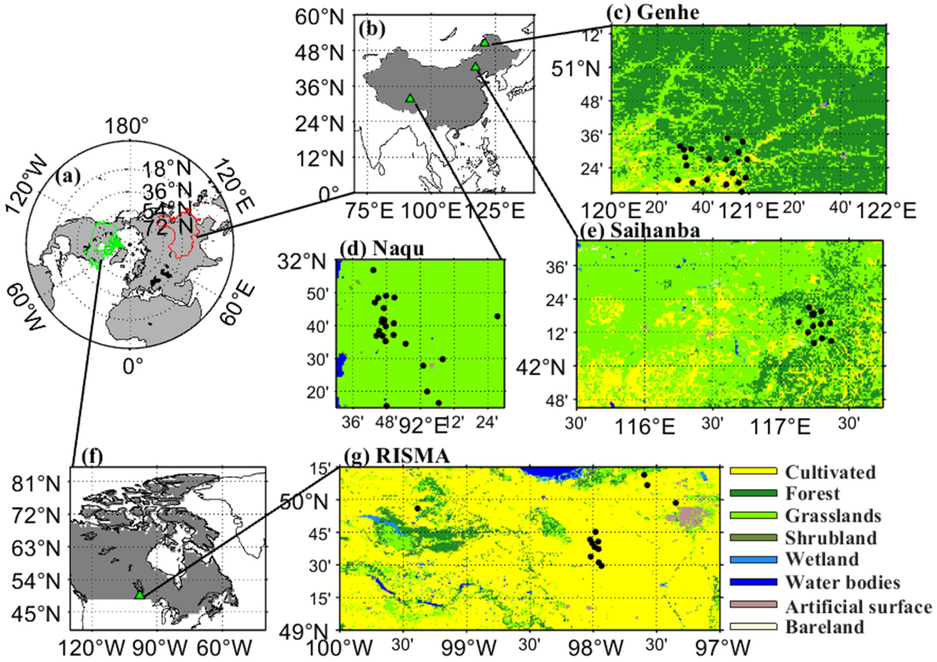
Figure 1.
Study area in Northern Hemisphere (a). Land cover map and distribution of in situ sites over the Genhe watershed (c), Saihanba (e), and Naqu (d) in China (b), and the RISMA network (g) in Canada (f).
Figure 1.
Study area in Northern Hemisphere (a). Land cover map and distribution of in situ sites over the Genhe watershed (c), Saihanba (e), and Naqu (d) in China (b), and the RISMA network (g) in Canada (f).
Figure 2.
Time series of boxplots of SSIS1 at VH polarization over the Genhe watershed (a), Saihanba (b), Naqu (c), and RISMA (d). On each box, the green line indicates the median, and the bottom and top edges of the box indicate the 25th and 75th percentiles, respectively. The whiskers extend to the most extreme data points not considered outliers, and the outliers are plotted individually using the ‘+’ marker symbol in black.
Figure 3.
Same as in
Figure 2 but the boxplot of SSI
S1 at VV polarization.
Figure 3.
Same as in
Figure 2 but the boxplot of SSI
S1 at VV polarization.
Figure 4.
An example of time series of satellite SSIS1, FTI, and in situ soil temperature for cultivated land ((a), site 11), grassland ((b), site 18), and forest ((c), site 2) over the Genhe watershed. Red line with red circle and red plus symbol are the SSI at VV and VH polarization, respectively. Black line with black circle and black plus symbol are the soil temperature and FTI, respectively.
Figure 5.
Scatters between SSI and FTI from simulation data. Black circles represent the simulation data.
Figure 5.
Scatters between SSI and FTI from simulation data. Black circles represent the simulation data.
Figure 6.
An example of scatters between SSIS1 and FTI from satellite data for cultivated land ((a), site 12), grassland ((b), site 3), and forest ((c), site 17) over the Genhe watershed. Black circles represent the satellite data.
Figure 6.
An example of scatters between SSIS1 and FTI from satellite data for cultivated land ((a), site 12), grassland ((b), site 3), and forest ((c), site 17) over the Genhe watershed. Black circles represent the satellite data.
Figure 7.
Scatter plot between the SSIS1 and SSInew both considering (d–f) and not considering (a–c) the LAI for cultivated land ((a,d), site 12), grassland ((b,e), site 3), and forest ((c,f), site 17) over the Genhe watershed.
Figure 7.
Scatter plot between the SSIS1 and SSInew both considering (d–f) and not considering (a–c) the LAI for cultivated land ((a,d), site 12), grassland ((b,e), site 3), and forest ((c,f), site 17) over the Genhe watershed.
Figure 8.
An example of the SSInew histogram at site 24 during late autumn to early spring.
Figure 8.
An example of the SSInew histogram at site 24 during late autumn to early spring.
Figure 9.
The classification accuracies of F/Tnew at each site from June 2017 to May 2019 in the Genhe watershed.
Figure 9.
The classification accuracies of F/Tnew at each site from June 2017 to May 2019 in the Genhe watershed.
Figure 10.
Time series of the SSIS1B, in situ soil moisture and ERA5-land snow depth at site MS3527 over the Naqu area. (a) Time series of the SSIS1 (black line marked with a black circle) and in situ soil moisture (blue dashed line); (b) time series of ERA5-land snow depth.
Figure 10.
Time series of the SSIS1B, in situ soil moisture and ERA5-land snow depth at site MS3527 over the Naqu area. (a) Time series of the SSIS1 (black line marked with a black circle) and in situ soil moisture (blue dashed line); (b) time series of ERA5-land snow depth.
Figure 11.
Time series of the SSInew, threshold of SSInew, in situ soil and ERA5-land air temperature data at site MB3 over the RISMA area.
Figure 11.
Time series of the SSInew, threshold of SSInew, in situ soil and ERA5-land air temperature data at site MB3 over the RISMA area.
Figure 12.
Comparison examples of the spatial distribution of SSIS1B, SSInew, the F/T state retrieved from the SSIS1B, SSInew, and the ERA5-land air temperature over Genhe watershed on 24 October 2018, 5 November 2018, respectively. (SSIS1B: (a,f); SSInew: (b,g); F/TS1B: (c,h); F/Tnew: (d,i); ERA5-land air temperature: (e,j).
Figure 13.
Time series of F/Tnew (first line), F/TS1B (second line) and air temperature over the Genhe watershed area from 24 October 2018 to 5 November 2018.
Figure 13.
Time series of F/Tnew (first line), F/TS1B (second line) and air temperature over the Genhe watershed area from 24 October 2018 to 5 November 2018.
Figure 14.
Same as
Figure 13 but over the Saihanba area from 10 November 2019 to 22 November 2019.
Figure 14.
Same as
Figure 13 but over the Saihanba area from 10 November 2019 to 22 November 2019.
Figure 15.
Same as
Figure 13 but over the RISMA area from 5 March 2019 to 17 March 2019.
Figure 15.
Same as
Figure 13 but over the RISMA area from 5 March 2019 to 17 March 2019.
Figure 16.
The histogram and spatial distribution of the root mean square error (RMSE) between SSInew and SSIS1 of the nonlinear regression model shown in Equation (11) over the Genhe watershed (a,b), Saihanba (c,d), Naqu (e,f), and RISMA (g,h) areas.
Figure 16.
The histogram and spatial distribution of the root mean square error (RMSE) between SSInew and SSIS1 of the nonlinear regression model shown in Equation (11) over the Genhe watershed (a,b), Saihanba (c,d), Naqu (e,f), and RISMA (g,h) areas.
Figure 17.
Two examples of the scatter plot among the SSIS1B, FTI, LAI, and SSInew with lower RMSE (a–c) and higher RMSE (d–f) from the Genhe watershed.
Figure 17.
Two examples of the scatter plot among the SSIS1B, FTI, LAI, and SSInew with lower RMSE (a–c) and higher RMSE (d–f) from the Genhe watershed.
Figure 18.
Comparison of 5 cm soil temperature between S1B overpass time (22:00) and AMSR2 overpass time of the descending orbit (1:30) over cultivated (a), grassland (b), and forest (c) in the Genhe watershed.
Figure 18.
Comparison of 5 cm soil temperature between S1B overpass time (22:00) and AMSR2 overpass time of the descending orbit (1:30) over cultivated (a), grassland (b), and forest (c) in the Genhe watershed.
Figure 19.
A comparison of thawed (a), frozen (b) and total (c) accuracies between F/Tnew and F/Tnew_noLAI.
Figure 19.
A comparison of thawed (a), frozen (b) and total (c) accuracies between F/Tnew and F/Tnew_noLAI.
Figure 20.
The frozen days of F/Tnew (a) and F/Tnew_noLAI (b) from June 2017 to May 2018 over the Genhe watershed area as an example.
Figure 20.
The frozen days of F/Tnew (a) and F/Tnew_noLAI (b) from June 2017 to May 2018 over the Genhe watershed area as an example.
Figure 21.
Comparison of thawed (a), frozen (b), and total (c) accuracies between F/TS1 and F/Tnew at a 1 km resolution.
Figure 21.
Comparison of thawed (a), frozen (b), and total (c) accuracies between F/TS1 and F/Tnew at a 1 km resolution.
Figure 22.
Comparisons of thawed (a), frozen (b), and total (c) accuracies between F/TAMSR2 and F/Tnew at the site level.
Figure 22.
Comparisons of thawed (a), frozen (b), and total (c) accuracies between F/TAMSR2 and F/Tnew at the site level.
Figure 23.
Frozen days calculated from the F/Tnew (a) at 1 km and F/TAMSR2 (b) at 25 km from June 2017 to May 2018.
Figure 23.
Frozen days calculated from the F/Tnew (a) at 1 km and F/TAMSR2 (b) at 25 km from June 2017 to May 2018.
Table 1.
Coordinates and land cover type of the in situ sites.
Table 1.
Coordinates and land cover type of the in situ sites.
| Area | Site Name | Lat (°) | Long (°) | Land Cover | Site Name | Lat (°) | Long (°) | Land Cover |
|---|
| Genhe | Site 1 | 50.507 | 120.529 | Grasslands | Site 17 | 50.451 | 120.987 | Forest |
| Site 2 | 50.451 | 120.711 | Forest | Site 18 | 50.327 | 120.484 | Grasslands |
| Site 3 | 50.448 | 120.834 | Grasslands | Site 19 | 50.329 | 120.696 | Cultivated |
| Site 5 | 50.413 | 120.547 | Grasslands | Site 20 | 50.311 | 120.589 | Cultivated |
| Site 9 | 50.556 | 120.955 | Grasslands | Site 24 | 50.309 | 120.927 | Cultivated |
| Site 11 | 50.301 | 120.836 | Cultivated | Site 26 | 50.256 | 120.948 | Cultivated |
| Site 12 | 50.367 | 120.883 | Cultivated | Site 27 | 50.529 | 120.499 | Grasslands |
| Site 14 | 50.511 | 120.581 | Grasslands | Site 28 | 50.463 | 120.537 | Grasslands |
| Site 15 | 50.575 | 120.843 | Forest | Site 29 | 50.341 | 120.977 | Forest |
| Site 16 | 50.492 | 120.926 | Forest | | | | |
| Saihanba | A3 | 42.312 | 117.242 | Grasslands | P8 | 42.311 | 117.233 | Forest |
| A5 | 42.309 | 117.236 | Grasslands | P9 | 42.249 | 117.294 | Grasslands |
| A6 | 42.308 | 117.241 | Grasslands | P10 | 42.255 | 117.359 | Forest |
| A7 | 42.305 | 117.231 | Grasslands | P11 | 42.201 | 117.199 | Forest |
| A11 | 42.307 | 117.233 | Forest | P12 | 42.236 | 117.236 | Grasslands |
| P2 | 42.351 | 117.207 | Forest | P13 | 42.164 | 117.302 | Forest |
| P6 | 42.367 | 117.296 | Forest | P15 | 42.135 | 117.242 | Forest |
| P7 | 42.261 | 117.131 | Forest | P16 | 42.149 | 117.371 | Forest |
| Naqu | BC07 | 31.274 | 92.109 | Grasslands | MS3513 | 31.677 | 91.842 | Grasslands |
| BC08 | 31.332 | 92.041 | Grasslands | MS3518 | 31.661 | 91.794 | Grasslands |
| C1 | 31.683 | 91.771 | Grasslands | MS3523 | 31.639 | 91.754 | Grasslands |
| C3 | 31.614 | 91.774 | Grasslands | MS3527 | 31.614 | 91.739 | Grasslands |
| C4 | 31.618 | 91.841 | Grasslands | MS3533 | 31.586 | 91.793 | Grasslands |
| CD01 | 31.712 | 92.458 | Grasslands | MS3545 | 31.573 | 91.912 | Grasslands |
| CD07 | 31.495 | 92.132 | Grasslands | MS3603 | 31.259 | 91.799 | Grasslands |
| F4 | 31.698 | 91.773 | Grasslands | MSNQRW | 31.463 | 92.017 | Grasslands |
| F5 | 31.693 | 91.786 | Grasslands | P1 | 31.782 | 91.729 | Grasslands |
| MS3475 | 31.946 | 91.721 | Grasslands | P10 | 31.807 | 91.845 | Grasslands |
| MS3494 | 31.805 | 91.749 | Grasslands | P11 | 31.815 | 91.795 | Grasslands |
| MS3501 | 31.754 | 91.782 | Grasslands | | | | |
| RISMA | MB1 | 49.562 | −98.019 | Cultivated | MB8 | 49.752 | −97.982 | Cultivated |
| MB2 | 49.492 | −97.933 | Cultivated | MB9 | 49.694 | −98.024 | Cultivated |
| MB3 | 49.519 | −97.956 | Cultivated | MB10 | 49.975 | −97.348 | Cultivated |
| MB4 | 49.636 | −97.988 | Cultivated | MB11 | 50.111 | −97.573 | Cultivated |
| MB5 | 49.621 | −97.957 | Cultivated | MB12 | 50.189 | −97.598 | Cultivated |
| MB6 | 49.678 | −97.959 | Cultivated | MB13 | 49.932 | −99.387 | Cultivated |
| MB7 | 49.665 | −98.007 | Cultivated | | | | |
Table 2.
Detailed information on S1 data over the four study areas. Number means the number of S1 SAR images during the time period.
Table 2.
Detailed information on S1 data over the four study areas. Number means the number of S1 SAR images during the time period.
| Area | S1A/S1B | Time Period | Number | Overpass Time |
|---|
| Genhe watershed | S1B | June 2017–May 2019 | 55 | 22:10 |
| Saihanba | S1B | August 2018–December 2019 | 33 | 22:20 |
| Naqu | S1A | January 2018–December 2019 | 59 | 23:50 |
| RISMA | S1B | January 2018–December 2019 | 57 | 00:23 |
Table 3.
The coefficients in Equation (5) over four study areas.
Table 3.
The coefficients in Equation (5) over four study areas.
| Area | a | b | c |
|---|
| Genhe watershed | −0.4552 | −44.3366 | 160.5139 |
| Saihanba | −0.3668 | −35.4591 | 129.0621 |
| Naqu | −0.279 | 40.1433 | 35.5872 |
| RISMA | −0.2266 | −3.3469 | 60.7911 |
Table 4.
Input parameters in the simulation of the radar backscattering coefficient and passive microwave Tb. RMS height indicates root mean square height. CL means correlation length.
Table 4.
Input parameters in the simulation of the radar backscattering coefficient and passive microwave Tb. RMS height indicates root mean square height. CL means correlation length.
| Simulation | Frequency (GHz) | Theta (°) | Soil Moisture (m3/m3) | Soil Temperature (°C) | RMS Height (cm) | CL (cm) | Sand Content
(%) | Clay Content
(%) |
|---|
| Radar | 5.406 | 40 | 0.02–0.44 | −50~50 | 2 | 20 | 40 | 30 |
| Passive | 6.925 | 55 | 0.02–0.44 | −50~50 | 2 | 20 | 40 | 30 |
| 36.5 |
Table 5.
Classification accuracy (%) statistics for F/Tnew over four study areas.
Table 5.
Classification accuracy (%) statistics for F/Tnew over four study areas.
| Area | F_Right | T_Right | Total_Right |
|---|
| Genhe watershed | 93.64 | 93.19 | 93.29 |
| Saihanba | 93.85 | 89.08 | 90.79 |
| Naqu | 93.13 | 85.77 | 88.53 |
| RISMA | 85.24 | 90.2 | 88.1 |
Table 6.
Total classification accuracy (%) statistics for F/Tnew and F/Tnew_noLAI.
Table 6.
Total classification accuracy (%) statistics for F/Tnew and F/Tnew_noLAI.
| | Area | Cultivated | Grassland | Forest |
|---|
| F/Tnew_noLAI | Genhe | 88.66 | 88.23 | 86.16 |
| Saihanba | / | 91.3 | 90.22 |
| Naqu | / | 86.4 | / |
| RISMA | 86.87 | / | / |
| F/Tnew | Genhe | 92.24 | 93.36 | 93.79 |
| Saihanba | / | 91.53 | 90.34 |
| Naqu | / | 88.53 | / |
| RISMA | 88.1 | / | / |
Table 7.
Classification accuracy (%) statistics for F/TS1 and F/Tnew.
Table 7.
Classification accuracy (%) statistics for F/TS1 and F/Tnew.
| | Area | FF | FT | TT | TF | F_Right | T_Right | Total_Right |
|---|
| F/TS1 | Genhe | 357 | 28 | 486 | 55 | 92.73 | 89.83 | 91.04 |
| Saihanba | 221 | 16 | 229 | 62 | 93.25 | 78.69 | 85.23 |
| Naqu | 558 | 38 | 555 | 206 | 93.62 | 72.93 | 82.02 |
| RISMA | 236 | 60 | 365 | 80 | 79.73 | 82.02 | 81.11 |
| F/Tnew | Genhe | 368 | 17 | 505 | 36 | 95.58 | 93.35 | 94.28 |
| Saihanba | 221 | 16 | 242 | 49 | 93.25 | 83.16 | 87.69 |
| Naqu | 552 | 44 | 649 | 112 | 92.62 | 85.28 | 88.5 |
| RISMA | 247 | 49 | 417 | 28 | 83.45 | 93.71 | 89.61 |
Table 8.
Classification accuracy (%) statistics for F/TAMSR2 and F/Tnew.
Table 8.
Classification accuracy (%) statistics for F/TAMSR2 and F/Tnew.
| | Area | FF | FT | TT | TF | F_Right | T_Right | Total_Right |
|---|
| F/TAMSR2 | Genhe | 4529 | 725 | 6897 | 134 | 86.2 | 98.09 | 93.01 |
| Saihanba | 2262 | 311 | 3819 | 392 | 87.91 | 90.69 | 89.64 |
| Naqu | 4868 | 513 | 5958 | 1024 | 90.47 | 85.33 | 87.57 |
| RISMA | 2891 | 795 | 5083 | 386 | 78.43 | 92.94 | 87.1 |
| F/Tnew | Genhe | 4888 | 366 | 6555 | 476 | 93.03 | 93.23 | 93.29 |
| Saihanba | 2823 | 189 | 4353 | 539 | 93.73 | 88.98 | 90.79 |
| Naqu | 6729 | 541 | 8136 | 1384 | 92.56 | 85.46 | 88.53 |
| RISMA | 3273 | 570 | 5088 | 559 | 85.17 | 90.1 | 88.1 |


 ,
, 


