Multi-Temporal LiDAR and Hyperspectral Data Fusion for Classification of Semi-Arid Woody Cover Species

Abstract

Mapping the spatial distribution of woody vegetation is important for monitoring, managing, and studying woody encroachment in grasslands. However, in semi-arid regions, remotely sensed discrimination of tree species is difficult primarily due to the tree similarities, small and sparse canopy cover, but may also be due to overlapping woody canopies as well as seasonal leaf retention (deciduous versus evergreen) characteristics. Similar studies in different biomes have achieved low accuracies using coarse spatial resolution image data. The objective of this study was to investigate the use of multi-temporal, airborne hyperspectral imagery and light detection and ranging (LiDAR) derived data for tree species classification in a semi-arid desert region. This study produces highly accurate classifications by combining multi-temporal fine spatial resolution hyperspectral and LiDAR data (~1 m) through a reproducible scripting and machine learning approach that can be applied to larger areas and similar datasets. Combining multi-temporal vegetation indices and canopy height models led to an overall accuracy of 95.28% and kappa of 94.17%. Five woody species were discriminated resulting in producer accuracies ranging from 86.12% to 98.38%. The influence of fusing spectral and structural information in a random forest classifier for tree identification is evident. Additionally, a multi-temporal dataset slightly increases classification accuracies over a single data collection. Our results show a promising methodology for tree species classification in a semi-arid region using multi-temporal hyperspectral and LiDAR remote sensing data.

1. Introduction

Encroachment of woody vegetation into grasslands occurs worldwide with known implications to ecosystem health [1,2,3,4]. Various studies have shown an association between woody encroachment and ecosystem degradation with consequences to carbon and hydrological cycles, decreased socioeconomic potential, vegetation productivity, habitat quality of wild herbivores and increased erosion [4,5,6,7,8,9,10,11]. Therefore, mapping the spatial distribution of woody vegetation species is an important requirement for sustainable vegetation management and scientific research [12,13,14,15,16,17,18]. Since land management practices for planning, treating, monitoring, and evaluation are often based on individual species, mapping vegetation distribution must also be on an individual level [19,20]. Mapping species specific distribution can aid in restoration and protection efforts and improve understanding of complex species interactions and overall distributions [21,22,23,24,25,26]. Accurately creating species specific maps can give us detailed knowledge about vegetation species composition, distribution, cover and density which provide a base for management decisions and directly influence policy [27,28,29,30,31,32]. Ground based measurements are time consuming, labor intensive, and require economic resources, while remote sensing derived measurements are an excellent alternative for providing efficient, low cost spatially explicit data [12,13,17,33,34,35]. Several studies have utilized various sensors such as passive multi-spectral and hyperspectral sensors, active light detection and ranging (LiDAR) and synthetic aperture radar (SAR) systems [16,17]. All these sensors provide different information that allow for estimation of biophysical parameters and tree species classification [16,17].

Studies have widely utilized multi-spectral sensors with varying spatial resolutions that offer different levels of detail but have not produced suitable accuracies when attempting to discriminate tree species [36]. Utilizing an object-based image analysis (OBIA) on 4 m multi-spectral Ikonos imagery, Kim et al. [37,38] achieved an 83% overall accuracy but was limited to three forest types and non-forested areas. A fine spatial resolution dataset can delineate some forest tree species such as presented in the study by Franklin and Ahmed [39] where OBIA and machine learning classification was used with unmanned aerial system (UAS) images to delineate five classes of tree species, resulting in an accuracy of 78%. High spectral resolution datasets are required to capture the complex variability of species spectral reflectance characteristics [40]. Utilization of hyperspectral sensors has been increasing as they offer more detailed spectral information about land surface characteristics compared to multi-spectral sensors [36,41]. A study carried out by Dian et al. [42] used the Compact Airborne Spectrographic Imager hyperspectral data in a support vector machine (SVM) classifier resulting in an overall accuracy of 86% for four woody species. Relying on spectral signals alone for species classification applications has its limitations due to penetrable canopies, multiple scattering, spectral mixing, and bright soil reflectance influences [43].

The use of LiDAR sensors to produce three-dimensional vegetation modelling offers an accurate method for measuring tree structural attributes [44]. Fusing airborne LiDAR and hyperspectral imagery is an advanced method that provides vertical and horizontal vegetation details that improve species specific distinction and classification confidence [24,44,45,46]. The fusion of datasets can provide complementary and synergistic capabilities for earth monitoring programs to produce vegetation land classification cover maps over large areas with species differentiation [24,43,47]. Hyperspectral datasets provide fine spectral resolution for retrieval of plant functional traits represented by vegetation indices while LiDAR provides tree structural attributes [44]. Incorporating LiDAR datasets increases classification accuracies by providing supportive structural information when optical hyperspectral remote sensing data is limited due to spectral mixing from bright background soils with sparse canopy cover [48,49,50]. Classification studies in forest ecosystems such as boreal, tropical, and temperate, have shown the possibilities of using a fusion of reflectance data and LiDAR datasets to improve distinguishing multiple species for classification estimates [36,51,52]. Asner et al. [51] found error rates of 18.6% or less when combining LiDAR structural data and unique spectroscopic signal for tree species detection within a terrestrial ecosystem. A study carried out by Ballanti et al. [53] explored hyperspectral and LiDAR data to classify 8 vegetation species using pixel/object-based approaches in random forest (RF) and SVM classifiers resulting in overall accuracies above 90% for all classifications. Another study carried out by Dalponte et al. [36] compared various combinations of LiDAR, hyperspectral, and multi-spectral data for tree species identification using pixel-based RF/SVM classifiers that resulted in accuracies from 85% to 93% with decreased accuracies with increased classes.

In arid or semi-arid regions, small sparse vegetation and bright (high albedo) soil backgrounds make it hard to delineate vegetation species through remotely sensed satellite images [19,20]. LiDAR and hyperspectral sensors on board UAS platforms present new technology that offers reduced cost for high spatial and spectral resolution data that are needed for ecological research [19,20]. Some efforts carried out by Sankey et al. [19,20] highlight the potential of utilizing high spatial resolution LiDAR and hyperspectral sensors on UAS drones for dryland vegetation species classification. Their study achieved overall classification accuracies ranging from 84% to 89% for four vegetation classes when performing maximum likelihood, RF, and SVM classifications, although the approach was limited to a small spatial extent (<100 ha) due to flight time limitations and USA Federal Aviation Administration (FAA) line of sight restrictions. More research by Dashti et al. [48] created regional scale maps (23,900 ha) using an integrated LiDAR-hyperspectral approach for classifying three xeric and mesic tree species resulting in accuracies of 60% to 89% with limitations in the mesic classes and low spatial resolutions of 17 km.

The main objective of this paper is to create a framework for producing a species-specific woody vegetation map including five of the most abundant woody species in a large semi-arid region by utilizing a fusion of simultaneously acquired airborne LiDAR and high spatial resolution hyperspectral data to improve classification accuracies. Specifically, we will: (1) create spectral vegetation indices from hyperspectral reflectance bands, create canopy height models derived from raw LiDAR point clouds, and use the data for woody species classification, then (2) assess classifier performance and lastly (3) assess the classifier model, important metrics in the model, and training data combinations. This study builds on prior research studies focused on local scales utilizing similar? resolution datasets for species-specific classifications [19,20,40,48,54].

2. Materials and Methods

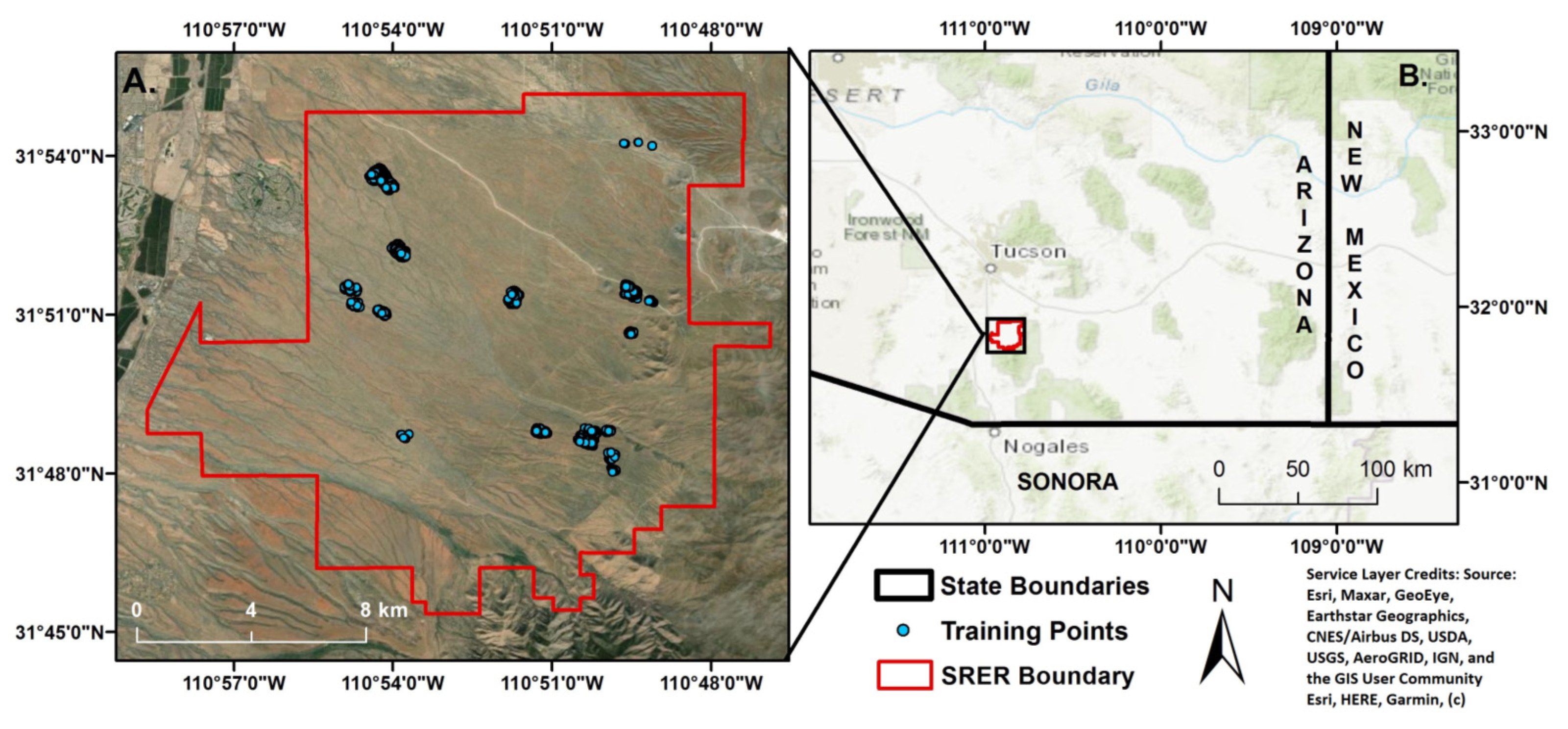
2.1. Study Area

This study was conducted about 80 km south of Tucson, Arizona, United States at the Santa Rita Experimental Range (SRER) (Figure 1). Between 1902 and 1988, SRER was managed by the United States Department of Agriculture Forest Service until the University of Arizona College of Agriculture and Life Sciences took over administration to support extensive ecological research as the longest active rangeland research facility in the United States. The area encompasses 21,000 hectares of semi-arid desert with an elevation gradient from 900 m in the northwest to 1400 m in the southwest. SRER has an average yearly temperature of 20 degrees Celsius and a bimodal precipitation distribution with rainfall events during summer and winter months averaging 275 to 450 mm a year.

The study area is characterized by gently sloped alluvial fans and small areas of precipitous stony hills and isolated buttes [55]. The current vegetation regime is a woody grass savanna with a mixture of scrubs, cacti, succulents, and other herbaceous species [56,57]. Higher elevations consist of savanna woodland while lower elevation physiognomy is desert scrub. Some common trees and shrubs within the study area include blue palo verde (Cercidium floridum (Benth)), velvet mesquite (Prosopis velutina (Woot.)), creosote (Larrea tridentata (Sesse & Moc.) Cov.), and graythorn (Ziziphus obtusifolia (Hook. ex Torr. & Gray) Gray) with an abundance of cacti such as prickly pear (Opuntia engelmanni Salm-Dyck) and various cholla (Cylindropuntia) species (Opuntia spinisior (Engelm.) Toumey, Opuntia fulgida Engelm).

2.2. Raw Data

This study utilized datasets captured by both manned and unmanned aircraft systems (MAS and UAS). Hyperspectral and LiDAR data were collected by the National Ecological Observatory Network (NEON), while high spatial resolution digital color images were collected using various UASs. NEON is funded by the National Science Foundation (NSF) to collect 30 years of long-term open access ecological data for understanding, predicting, and observing U.S. ecosystem change. NEON airborne remote sensing surveys are conducted during peak greenness (90% maximum foliage) seasons at various sites on a national level, using the Airborne Observation Platform (AOP) installed on a light MAS. The NEON AOP collected three years of hyperspectral and LiDAR at the SRER during 2017 (collection data: 24–30 August), 2018 (collection data: 24–28 August), and 2019 (collection data: 1–13 September). Flight surveys were conducted at a low altitude (1000 m AGL) and utilized a minimum of 10 km² area flight box design (survey boundaries) to produce consistent nominal 1 m spatial resolution datasets. Data products were published categorically by levels 1, 2, and 3 (L1, L2, L3) based on the complexity of processing steps. (https://www.neonscience.org/data-collection/airborne-remote-sensing, accessed on 3 December 2021). Level 1 point cloud and level 3 hyperspectral data products were used in this study. Each year had some data gaps and bad pixels due to cloud cover and were excluded from the analysis.

2.2.1. Hyperspectral Data

The AOP imaging spectrometer (NIS) is a passive remote sensing instrument based on the Next Generation Airborne Visible/Infrared Imaging Spectrometer (NG-AVIRIS) developed by NASA’s Jet Propulsion Laboratory (JPL). Level 3 NIS products are atmospherically corrected, orthorectified, scaled by 10,000, and stored in HDF5 format. ATCOR was used to atmospherically correct data products and orthorectified using the UTM projection/ITRF00 datum coordinate system [58]. The NIS level 3 algorithm accounts for sensor position, topography, solar positions, and atmospheric scattering resulting in a NIS level 3 surface reflectance product that has 1 m resolution and is distributed as 1 km × 1 km tiles. Four hundred and twenty-six spectral bands were then subset and converted into thirty-eight tiff reflectance bands to derive spectral indices based on the strongest signal with the least amount of noise.

2.2.2. Point Cloud Data

The AOP operates three commercial LiDAR systems, two Optech Geminis and a Riegle LMS-Q780. These systems receive and transmit high pulse repetition frequencies (PRF) to provide detailed terrain sampling [59]. The Optech Gemini sensors have been active since 2013 and can return reliable point cloud data at a maximum of 100,000 PRF (100 kHz). The Riegl LMS-Q780, active since 2018, operates at a maximum of 400,000 PRF (400 kHz). The LiDAR adjacent flight lines were designed to have a 30% overlap and at least 36° full scan angle with each laser possibly generating multiple returns. PRF’s between 100,000 and 400,000 can produce 2–8 laser pulses touching the landscape every square meter. A point density of 64 points per square meter can be obtained if the ground cover produces multiple returns and overlapping areas can produce double pulses or points. The level 1 LiDAR products are published in the American Society for Photogrammetry and Remote Sensing (ASPRS) journal as an unclassified orthorectified three-dimensional point cloud in LAS meters file format.

2.2.3. Drone Images

We used seventeen high-resolution orthomosaicked images from previous UAS flights piloted by Gillan et al. [60] in 2019 using the DJI Phantom 4 RTK. The flying height was 38 m above ground level (AGL), which resulted in plot sizes from 1.6 to 7.1 ha and a spatial resolution of 1 cm. Most of the images collected were in the southeast section of the SRER and represent the vegetation dynamics in a slightly higher elevation gradient of the range. In 2021, using the DJI Mavic2 Enterprise Dual, we collected high resolution RGB images over six additional sites in the northwest section of the study area to incorporate the different abundant vegetation species within the region for training and validation data detection and selection (Figure S1). To cover a larger area, we flew at a height of 90 m, which resulted in a spatial resolution of 2 cm and plot sizes from 26.9 to 30.9 ha. Each scene collected by the drone was orthomosaicked using Agisoft PhotoScan (version 1.4.4) to create a georeferenced orthomosaicked RGB image. A total of 23 RGB images were used for this study with plot sizes ranging from 1.6 to 30.9 ha and spatial resolutions of <s2 cm. The difference in UAS drone imagery collection time was not a limitation due to slow tree growth patterns and their simple usage as a visualization aid to delineate tree species locations.

2.3. Data Processing

All data were processed through the R programming language and open-source software in RStudio [61]. We utilized parallel processing on large datasets of hyperspectral and LiDAR to produce high spatial resolution classifications of vegetation species. Three years of data were clipped, mosaicked, and stacked to create overlapping raster stacks (Figure 2 and Figure 3). We used an optimal number of cores from 8–15 at a time to speed up processing without compromising or overwhelming performance and memory.

2.3.1. Indices

To optimize hyperspectral metrics and reduce spectral data dimension, 38 spectral bands were selected for this study. The bands chosen had the clearest variation in signals and were readily available for indices calculation appropriate for the study area. We calculated 12 vegetation indices highlighted in

Table 1. Band numbers, respective wavelengths, and vegetation indices that were used in the study with their respective formulas and the references. ρ is used to reference a specific band number that corresponds to a wavelength in nm.

HDF5 Band	TIFF Band	Wavelength (nm)	Indices	Equation
31	4	531	NDVI	$\frac{\rho 862-\rho 661}{\rho 862+\rho 661}$
35	5	551	NDWI	$\frac{\rho 1242-\rho 862}{\rho 1242+\rho 862}$
38	6	564	PRI	$\frac{\rho 551-\rho 531}{\rho 551+\rho 531}$
57	10	661	PRI2	$\frac{\rho 531-\rho 564}{\rho 531+\rho 564}$
59	11	671	SWIRI	$\frac{\rho 1648-\rho 1548}{\rho 1648+\rho 1548}$
67	13	711	SAVI	$1.5\left(\frac{\rho 862-\rho 661}{\rho 862+\rho 661+5000}\right)$
75	14	751	CACTI	$\frac{\rho 862-\rho 970}{\rho 862+\rho 970}$
97	16	862	CACTI2	$\frac{\rho 1070-\rho 970}{\rho 1070+\rho 970}$
119	17	970	MTCI	$\frac{\rho 751-\rho 711}{\rho 711+\rho 671}$
139	18	1070	CI	$\left(\frac{\rho 751}{\rho 711+\rho 751}\right)-1$
173	20	1242	CAI	$0.5\left[\left(\rho 2000+\rho 2210\right)-\rho 2134\right]10$
226	22	1508	NDNI	$\frac{\log \left(\frac{1}{\rho 1508}\right)-\log \left(\frac{1}{\rho 1678}\right)}{\log \left(\frac{1}{\rho 1508}\right)+\log \left(\frac{1}{\rho 1678}\right)}$
234	23	1548
254	25	1648
260	27	1678
324	32	2000
351	34	2134
366	36	2210

. Vegetation indices were developed based on biophysical and biochemical signals of various absorption features that aid in detecting and mapping vegetation species. Bands selected were derived from previous research based on differences in reflectance and absorption features that represent various plant species [62,63].

Vegetation indices (VI) were calculated to highlight vegetation canopy structure, chlorophyll content, water content, leaf area index, pigments, cellulose absorption and light use efficiency to improve discrimination of different species. The normalized difference vegetation index (NDVI) highlights green plants’ chlorophyll absorption of red light and reflectance or scattering of near-infrared (NIR) light [64]. The normalized difference water index (NDWI) was used to distinguish soil from vegetation features by utilizing NIR and short-wave infrared (SWIR) bands [64]. The soil adjusted vegetation index (SAVI) minimizes soil brightness influence on vegetation indices involving red and NIR wavelengths [65,66,67]. The normalized difference nitrogen index (NDNI) estimates canopy nitrogen (N) and lignin contents [68,69]. We used photochemical reflectance indices (PRI) 1 and 2 to assess short term changes in photosynthetic activity with their sensitivities to xanthophyll cycle pigment de-epoxidation state and photosynthetic efficiency [70,71,72,73]. CACTI 1 and 2 were indices developed to identify cacti vegetation using near-infrared signals and water absorption in larger landscapes using hyperspectral bands [74]. The MERIS Terrestrial Chlorophyll Index (MTCI) estimates chlorophyll content with a sensitivity to the red edge position by utilizing reflectance ratio within the wavelength range of 650–700 nm [75,76]. The cellulose absorption index (CAI) was used to account for non-photosynthetic vegetation cover and soil discrimination through depths of cellulose by selecting absorption features positioned at a water absorption feature shoulders within 2000 nm–2210 nm [75,76,77,78,79,80]. Chlorophyll index (CI) was used to measure the amount of chlorophyll in plants as an indicator of leafy vegetation health through selection of bands within the hyperspectral dataset red-edge sections [81,82,83]. To create a short-wave infrared index (SWIRI), near short wave infrared bands from 1648–1642 are used with 1548, 1620 or 1690 nm to detect moister sensitivity based on chlorophyll sensitivity to the fluctuations of plant moisture [80,84,85,86,87].

2.3.2. Canopy Height Model

LAS point cloud data were processed to create a digital terrain model (DTM) for canopy height model (CHM) calculation. Discrete LiDAR point clouds contain information on 3D coordinates of reflected laser energy locations. A digital terrain model (DTM) was created using the lidR [88] package for spatial interpolation by k-nearest neighbor (KNN) of 12 with an inverse-distance weighting (IDW) of 2 in RStudio [61]. The normalized DTM point cloud uses an algorithm that implements a point to raster (p2r) method for creating a denser collection of points resulting in a smoother CHM raster [61,88]. The CHM was created with a p2r of 0.25 and a cell resolution of 0.5 m for a model that best captured vegetation height.

2.3.3. Training Data

To validate the UAS hyperspectral data and to assess image classification outputs, plant canopies and target species of interest were geolocated and hand-delineated using field-based GPS data, an independent source of high-resolution imagery, and ground-based photographs. Accuracy assessment samples were individual pixels randomly selected within canopies across the various flight areas. A total of 3144 trees were selected within the high spatial resolution RGB drone images as training samples for the 5 most abundant woody species within the study area, bare ground, and herbaceous classes. Different dominant species were clearly identifiable through visual interpretation of the orthomosaic imagery, vegetation indices, and the CHMs. Additionally, individual geotagged images of trees during field visits were used to aid in species delineation. Reference points were created within visually defined canopy boundaries on the CHM and vegetation indices. Landscape patterns within all the georeferenced images and high spatial resolution drone images made it easy to identify different tree species.

2.3.4. Classification

Various classification algorithms were tested for this study including Random Forest (RF), Support vector machine (SVM), and a Classification and Regression Tree model (CART). Bare ground and herbaceous cover were classified in addition to five abundant woody species selected for the study including mesquite, palo verde, creosote, lotebush, and cacti. Although clearly not a woody species, we included cacti since it is one of the dominant species in this region. We conducted a comparative approach that compares classifiers and training sample combinations. Each classifier was compared using all available data and the classifier that resulted in the highest overall classification accuracy was used to compare training sample combinations. Visual assessments of indices and CHM imagery were used to find inconsistencies in the data that could influence the final classifications. Some datasets had missing data and/or sensor issues that resulted in a final product of a mosaicked classification (white spaces within the SRER boundaries—Figure S2). Years with obvious sensor issues were removed from the classifications which were then used to fill gaps in the highest overall accuracy classification with all data available.

CART

CART is an algorithm that was developed by Breiman et al. [89] but dates to the 1960s with Automatic Interaction Detection (AID) [90,91]. Models are represented as binary trees with a two-stage procedure and a no interaction responsive formula [92,93]. Decision trees (DT) are constructed by recursively splitting at a node based on the independent variable that resulted in the largest heterogeneous reduction in the dependent variable [90,91,92,93]. The CART model with a minimum of five observations to split a node was built through the Recursive Partitioning and Regression Trees “rpart” package [92,93].

SVM

SVM is a non-parametric classifier model based on statistical learning theory that calls a hyperplane discriminative line through kernel functions to maximize separation between classes and minimize the number of misclassification errors to a proportional quantity [94,95,96,97,98]. The data points used to measure the margin are closest to the hyperplane and are small in numbers [94,95,96]. The algorithm uses a penalizing cost-classification parameter and a function specific radial basis—gamma [99,100]. Models are based on training data with an implementation of matrix and formula interface with a factor dependent variable type (y) for classification [99,100]. A linear SVM model was created using the “e1071” package with parameters best fit for desert vegetation based on Ge et al. [101] which are 0.125 cost and 128 kappa [102,103,104,105,106].

RF

The RF classifier uses randomly selected training data to produce multiple decision trees for an ensemble classification [104,105,106]. Since the RF classifier does not overfit and is computationally efficient, the user-defined number of features and trees grown (N trees) at each node can be as large as possible [97,98,107,108,109]. Our study used a common error stabilizing N value of 500 trees within the R package “randomForest” [97,98,106,110,111].

2.4. Accuracy Assessment

Visual inspections were conducted of each classified image to compare results and assess possible errors. Additionally, a confusion matrixbased on a 5-k-fold cross validation accuracy assessment resulting in overall accuracy (OA), user accuracy (UA), producer accuracy (PA), and kappa was used to accept or reject each classification model and find the highest accuracy classification map. K-fold cross validation subsets the data by randomly choosing equal samples in each fold then using one-fold for validation and four for training [112,113]. The training and testing steps were repeated five times with different partitions to report averaged results [114,115,116,117]. Additionally, variable importance was measured using the mean decrease Gini (MDG) coefficient to assess the contribution of each variable to the classifier’s nodes and leaves homogeneity [118].

3. Results

Classifications were performed with all years of available data using RF, SVM, and CART classifiers. Each classifier was compared and the classifier with the highest overall accuracy was used to perform eight additional classifications with various combinations of datasets. Classification performance of each classifier model is shown in

Table 2. SVM, RF and CART Classifier Overall Accuracy, kappa and processing time in minutes.

All Years Indices + Lidar	SVM	RF	CART
OA	77.48	95.28	88.55
Kappa	72.14	94.17	85.88
Processing Time (min)	55.46	52.30	46.27

. The RF classifier was successful at achieving the highest classification OA of 95.28% and a kappa of 94.17% compared to the SVM and CART classifiers. The SVM classifier achieved the lowest OA of 77.48% and kappa of 72.14% compared to CART achieving an OA of 88.55% and kappa of 85.88%. We utilized the RF classifier to assess training data combinations and produce a final classification map due to it resulting in the highest OA and kappa.

3.1. Training Data Combinations

Classification iterations were conducted using the RF classifier with different combinations of mono- and multi-temporal data. The highest overall classification accuracy, 95.28%, was achieved by using data from all years, while removing the LiDAR data decreased the accuracy to 93.19%. The 2018 and 2019 classifications with LiDAR resulted in the same OA of 92.62% while 2017 dropped to 89.11% OA. Removing the LiDAR training dataset caused about a 3% or more decrease in yearly classification overall accuracies to 90.61%, 88.76%, and 87.78% for 2019, 2018, and 2017 (

Table 3. Training Data Combination OA and kappa.

Training Data Combinations	OA	Kappa
All Years Indices + Lidar	95.28	94.17
2019 Indices + Lidar	92.62	90.88
2018 Indices + Lidar	92.62	90.88
2017 Indices + Lidar	89.11	86.90
All Years Indices	93.19	91.57
2019 Indices	90.61	88.41
2018 Indices	88.76	86.99
2017 Indices	87.78	84.87

).

3.2. Classification Assessment

Visual assessment of the classification showed some issues of missing or misclassification due to raw data having empty data pixels, sensor issues, and weather impacts. Areas with misclassification based on sensors were removed and replaced by the next best classification.

The best classification with the highest overall accuracy of 95.28% OA and a kappa of 94.17% resulted in all classes with accuracies over 90% besides mesquite and lotebush which had accuracies in the 80 s with 88.03% and 86.12% (

Table 4. Shows error matrix and producer/user accuracies for classification iteration with the highest overall accuracy (All Years Indices + LiDAR) and the lowest overall accuracy (2017 Indices).

All Years Indices + LiDAR	Bare Ground	Grass	Mesquite	Cactus	Lotebush	Paloverde	Creosote	Sum	UA
Bare ground	365	2	0	1	0	0	0	368	99.18
Grass	5	287	0	1	2	0	2	297	96.63
Mesquite	0	0	397	1	32	5	2	437	90.85
Cactus	1	2	2	1068	1	3	1	1078	99.07
Lotebush	0	2	43	1	242	2	7	297	81.48
Paloverde	0	0	8	10	2	285	1	306	93.14
Creosote	0	1	1	5	2	0	350	359	97.49
Sum	371	294	451	1087	281	295	363	3142
PA	98.38	97.62	88.03	98.25	86.12	96.61	96.42
2017 Indices	Bare Ground	Grass	Mesquite	Cactus	Lotebush	Paloverde	Creosote	Sum	UA
Bare ground	351	4	0	10	0	0	3	368	95.38
Grass	8	249	5	14	6	1	14	297	83.84
Mesquite	0	3	370	1	50	8	5	437	84.67
Cactus	12	21	10	1022	0	9	4	1078	94.81
Lotebush	0	5	105	2	175	1	9	297	58.92
Paloverde	0	4	13	16	4	266	3	306	86.93
Creosote	13	5	2	10	3	1	325	359	90.53
Sum	384	291	505	1075	238	286	363	3142
PA	91.41	85.57	73.27	95.07	73.53	93.01	89.53

). The variables of greatest MDG were the CACTI, CI, CHM, NDWI, and NDVI. The 2018 CHM had the highest variable importance based on MDG with 2018 and 2019 CACTI, CACTI2, NDVI, and NDWI consecutively following in importance (

Table 5. MDG for classification iteration with the highest (All Years Indices + LiDAR) and lowest overall accuracy (2017 Indices).

All Years Indices + LiDAR	MDG	2017 Indices	MDG
CACTI_2019	131.3818	CACTI_2017	291.5153
CACTI_2018	128.0493	NDVI_2017	266.4296
CHM_2018	118.9476	CACTI2_2017	260.4622
CACTI2_2019	105.366	CI_2017	240.1875
CACTI2_2018	97.37399	NDWI_2017	168.1216
NDVI_2018	83.49702	SWIRI_2017	151.0334
CI_2018	75.12076	NDNI_2017	140.9909
NDVI_2019	74.52218	SAVI_2017	124.6892
NDWI_2019	71.98403	PRI2_2017	115.7335
NDWI_2018	61.93623	MTCI_2017	114.6043
NDNI_2018	58.84034	CAI_2017	86.10462
SWIRI_2019	55.42875	PRI_2017	72.31956
CI_2019	52.13248	CACTI_2017	291.5153
CAI_2019	51.43631	NDVI_2017	266.4296

).

4. Discussion

This study was performed to create a regional species-specific woody cover map in a semi-arid environment. We conducted a series of classifications with a scripted programming approach in an open-source software. In this study, SVM and CART classifiers were less successful in classifying woody species based on a k-fold validation of OA and kappa compared to the RF classifier. Results found that RF had an increased OA by about 18% compared to the SVM and 7% compared to the CART classifiers. RF MDG variable importance based on large numbers of trees and prevention of tree masking by other correlated inputs make it a powerfully effective approach for classifying woody tree species in an arid environment and assessing feature selection. Additionally, the number of user-defined required inputs are less for the RF classifier compared to the SVM classifier. Our results line up with similar remote sensing studies that compared various classifiers that resulted in RF with the highest OA compared to CART, SVM, and other classifiers [97,98,116,117,119]. Our RF classifier resulted in 8% higher OA accuracy when compared to a similar study carried out by Naidoo et al. [40] utilizing RF models to predict savanna ecosystem tree species. Our study utilized an open source R programming approach which makes it easily transferable to other larger areas with available data. Depending on data availability, Google Earth Engine (GEE) could be used apply the same methodology to larger areas and fast processing. Accuracy assessments will need to be performed to evaluate performance in other and larger areas.

To reduce processing time and noise while increasing vegetation delineation we utilize a vegetation index-based training dataset to reduce the number of bands or layers within the classifier and highlight vegetation processes [120,121,122,123]. Adding a layer of LiDAR derived CHMs for quantification of tree height provides a unique vegetation delineation to increase classification accuracy (Table 3, Figure 4). Utilizing both VI and CHM informs the classifier regarding different vegetation assets. Our study shows that tree species classification performance increases when a multiyear combination of structure and spectral information are informing the classifier [16,17,36,124,125,126]. Utilizing multiyear VI on their own resulted in good classifications with over 93.19% OA and 91.57% kappa but species delineation increased when CHM models were added to the predictor variables as OA of classifications increased by 3% (Table 3).

A similar study carried out by Sankey et al. [19] classifying four vegetation species within an arid and semi-arid region using a UAS derived LiDAR and hyperspectral data resulted in an OA of 84–89%. Compared to our study, lower OA were obtained with a smaller number of classes. Similarly, comparing our study to other studies utilizing LiDAR and hyperspectral data such as, Matsuki et al. [127] where they classified sixteen mixed forest types and Dalponte et al. [36] where they classified seven tree species in a mountainous region, resulted in 18% and 13% less OA with 82% and 77%.

MDG values show that spectral data contribute the most to classification accuracy, but structural tree height parameters further improve classification accuracies (Table 5). For our results, we conclude that the LiDAR derived CHM model is a useful compensation tool for minor loss or lack of information through spectral signals and utilizing VI training reduces the number of bands which reduces the number of features in the model for continued reduction in computation time and increase system capacity.

Additionally, we use a multi date training classification dataset that increased classification OA between about 3% and 7% with years 2019 and 2018 variables having the highest influence on classification accuracies (Table 3). Our results are in line with other studies using multi-temporal data for classifications utilizing UAS and non-UAS imagery. Classifications with multi-temporal datasets resulted in the highest OA with all mono-temporal classification resulting in the lowest OA.

Similar results from studies carried out by Weil et al. [128] and Grybas and Congalton [129] found the optimal multi-temporal training dataset was three dates with OA leveling off after three datasets. Our results reinforce the benefits of multi-temporal classification datasets in increasing classification OA compared to a single date. However, the achieved accuracy of the multi-temporal hyperspectral and Lidar dataset stack was only 3% lower than the best single-date classification (Table 3 and Figure 4). Wolter et al. [130] and Mickelson et al. [131] made similar observations based on multi-temporal/multi-spectral datasets resulting in improved classifications. In contrast, Key et al. [132] and Modzelewska et al. [54] found that multi-temporal datasets did not outperform mono date classifications based on their multi-spectra temporal datasets. The difference in results could indicate that collecting a single date spectral and structural remote sensing data at an optimal collection time during peak species contrast could provide similar results as multi-temporal spectral and structural datasets.

We found that VI’s CACTI, NDVI, NDWI, and CI combined with CHMs had the highest influence on the RF classifier during prediction (Table 5). CACTI, NDVI, and NDWI utilize the NIR bands while CI have a variation of NIR and RED bands similarly to the NDVI. Additionally, NDWI includes the SWIR, suggesting that red, NIR, SWIR bands, and CHM increased the capacity to delineate tree species in a semi-arid region. Confusion matrices indicate that the lowest classification OAs were measured for mesquite and lotebush which is supported by the similarities in their spectral signal and canopy height (Table 4, Figure 3 and Figure 5).

Utilizing multi-temporal datasets can introduce challenges to the classification process. Different stages of plant development or phenology during collection time, sensor noise, and weather-related data gaps are a few reasons for classification uncertainty. As shown in Figure S2, there are differences in tree positions, the number of trees/shrubs and weather leather data gaps, which can introduce error when using the same polygons for all datasets. These differences are possibly based on differences in NEON sensor characteristics. Studies have shown these differences influence results when using high spatial resolution images [133,134,135,136,137]. Ferreira et al. [135] had to adjust polygons at each tree sample for resampled WorldView images with varying resolutions between 0.30 and 1.2 m. Our results coincide with prior studies based on NEON 2017 having the lowest quality dataset and lowest influence on the RF forest model. Additionally, NEON 2019 and 2018 had better quality data and in turn resulted in the highest variable importance and strongest predictors within the RF model (Figures S2 and S5, Table 5). The increase in vegetation signal could be due to increased precipitation events during data acquisition in 2019 and 2018 compared to 2017 (Figure 5). Additionally, 2018 CHM had the highest influence based on the Riegl LMS-Q780 LiDAR sensor’s capacity to produce high pulse repetition frequencies (PRF) and return reliable point cloud data at 400 kHz compared to the 2017 and 2019 sensor Optech Gemini LiDAR sensors that produced point cloud data at a maximum 100 kHz. Lastly, cloud cover and sensor noise at specific wavelength bands produced misclassification and classification gaps (Figure S2).

5. Conclusions

This study compared prediction accuracy of modeling methods, various data types, and multi-temporal data for classifying dominant woody vegetation species in a semi-arid region. Our work has demonstrated the application of fine spatial resolution airborne multi-temporal LiDAR and hyperspectral data to effectively identify and classify woody vegetation species in a semi-arid desert region at the Santa Rita Experimental Range.

The results indicate that the best modelling method is the RF with all data types. The RF model results, with a combination of spectral and structural data from mono or multi temporal datasets, resulted in satisfying accuracies. LiDAR data fused with spectral data yielded the highest accuracy and incorporating multi-temporal datasets slightly improved classification accuracy estimates. The main source of misclassifications is in the confusion of lotebush and mesquite due to their similar signals of VI and CHM. Additional indices or data available when lotebush is blooming could help it from delineating from mesquite. To apply this method in other areas, an in situ inventory of tree and species locations are needed to aid in remote identification of tree species using UAS images. Additionally, auxiliary information or multi-temporal data of equal quality may be needed to further delineate tree species more accurately.

The results of this classification study are important in providing land managers and research scientists spatially explicit tree species maps to locate species specific woody encroachment and assess factors influencing woody encroachment [137,138,139,140,141,142]. Our study considers phenology and species traits to increase classification results by using NEON multi-temporal hyperspectral derived vegetation indices and LiDAR derived canopy height data that provide useful information for delineation of tree species in a semi-arid region. In general, the methodology detailed in this paper demonstrated the ability to perform computationally fast, accurate woody species classifications of larger areas. We also demonstrated that classification accuracies were affected by dataset proxies for vegetation dynamics, data phenological signal strength, data quality, and multi-temporal data availability.

References

1. Briggs, J.M.; Schaafsma, H.; Trenkov, D. Woody vegetation expansion in a desert grassland: Prehistoric human impact? J. Arid Environ. 2007, 69, 458–472. [Google Scholar] [CrossRef]
2. Barger, N.N.; Archer, S.R.; Campbell, J.L.; Huang, C.Y.; Morton, J.A.; Knapp, A.K. Woody plant proliferation in North American drylands: A synthesis of impacts on ecosystem carbon balance. J. Geophys. Res. Biogeosci. 2011, 116. [Google Scholar] [CrossRef]
3. Huxman, T.E.; Wilcox, B.P.; Breshears, D.D.; Scott, R.L.; Snyder, K.A.; Small, E.E.; Hultine, K.; Pockman, W.T.; Jackson, R.B. Ecohydrological implications of woody plant encroachment. Ecology 2005, 86, 308–319. [Google Scholar] [CrossRef]
4. Eldridge, D.J.; Bowker, M.A.; Maestre, F.T.; Roger, E.; Reynolds, J.F.; Whitford, W.G. Impacts of shrub encroachment on ecosystem structure and functioning: Towards a global synthesis. Ecol. Lett. 2011, 14, 709–722. [Google Scholar] [CrossRef]
5. Grover, H.D.; Musick, H.B. Shrubland encroachment in southern New Mexico, USA: An analysis of desertification processes in the American Southwest. Clim. Chang. 1990, 17, 305–330. [Google Scholar] [CrossRef]
6. Goudie, A.S. Human Impact on the Natural Environment; John Wiley & Sons: Hoboken, NJ, USA, 2018. [Google Scholar]
7. Pacala, S.W.; Hurtt, G.C.; Baker, D.; Peylin, P.; Houghton, R.A.; Birdsey, R.A.; Heath, L.; Sundquist, E.T.; Stallard, R.F.; Ciais, P.; et al. Consistent land-and atmosphere-based US carbon sink estimates. Science 2001, 292, 2316–2320. [Google Scholar] [CrossRef] [Green Version]
8. Pan, Y.; Birdsey, R.A.; Fang, J.; Houghton, R.; Kauppi, P.E.; Kurz, W.A.; Phillips, O.L.; Shvidenko, A.; Lewis, S.L.; Canadell, J.G.; et al. A large and persistent carbon sink in the world’s forests. Science 2011, 333, 988–993. [Google Scholar] [CrossRef] [Green Version]
9. Jackson, R.B.; Banner, J.L.; Jobbágy, E.G.; Pockman, W.T.; Wall, D.H. Ecosystem carbon loss with woody plant invasion of grasslands. Nature 2002, 418, 623–626. [Google Scholar] [CrossRef]
10. Wardle, D.A.; Bardgett, R.D.; Klironomos, J.N.; Setala, H.; Van Der Putten, W.H.; Wall, D.H. Ecological linkages between aboveground and belowground biota. Science 2004, 304, 1629–1633. [Google Scholar] [CrossRef]
11. David, J.A.; Kari, E.V.; Jacob, R.G.; Corinna, R.; Truman, P.Y. Pathways for Positive Cattle–Wildlife Interactions in Semiarid Rangelands. In Conserving Wildlife in African Landscapes: Kenya’s Ewaso Ecosystem; Smithsonian Contributions to Zoology: Washington, DC, USA, 2011; pp. 55–71. [Google Scholar] [CrossRef]
12. Mairs, J.W. The use of remote sensing techniques to identify potential natural areas in oregon. Biol. Conserv. 1976, 9, 259–266. [Google Scholar] [CrossRef]
13. Ghosh, A.; Fassnacht, F.E.; Joshi, P.K.; Koch, B. A framework for mapping tree species combining hyperspectral and LiDAR data: Role of selected classifiers and sensor across three spatial scales. Int. J. Appl. Earth Obs. Geoinf. 2014, 26, 49–63. [Google Scholar] [CrossRef]
14. Franklin, S.E. Remote Sensing for Sustainable Forest Management; CRC Press: Boca Raton, FL, USA, 2001. [Google Scholar] [CrossRef]
15. Lu, D.; Weng, Q. A survey of image classification methods and techniques for improving classification performance. Int. J. Remote Sens. 2007, 28, 823–870. [Google Scholar] [CrossRef]
16. Dalponte, M.; Bruzzone, L.; Gianelle, D. Fusion of hyperspectral and LIDAR remote sensing data for classification of complex forest areas. IEEE Trans. Geosci. Remote Sens. 2008, 46, 1416–1427. [Google Scholar] [CrossRef] [Green Version]
17. Mountrakis, G.; Im, J.; Ogole, C. Support vector machines in remote sensing: A review. ISPRS J. Photogramm. Remote Sens. 2011, 66, 247–259. [Google Scholar] [CrossRef]
18. Chopping, M.; Su, L.; Rango, A.; Martonchik, J.V.; Peters, D.P.; Laliberte, A. Remote sensing of woody shrub cover in desert grasslands using MISR with a geometric-optical canopy reflectance model. Remote Sens. Environ. 2008, 112, 19–34. [Google Scholar] [CrossRef]
19. Sankey, T.; Donager, J.; McVay, J.; Sankey, J.B. UAV lidar and hyperspectral fusion for forest monitoring in the southwestern USA. Remote Sens. Environ. 2017, 195, 30–43. [Google Scholar] [CrossRef]
20. Manfreda, S.; McCabe, M.F.; Miller, P.E.; Lucas, R.; Pajuelo Madrigal, V.; Mallinis, G.; Ben Dor, E.; Helman, D.; Estes, L.; Ciraolo, G.; et al. On the use of unmanned aerial systems for environmental monitoring. Remote Sens. 2018, 10, 641. [Google Scholar] [CrossRef] [Green Version]
21. Anderson, J.E.; Plourde, L.C.; Martin, M.E.; Braswell, B.H.; Smith, M.L.; Dubayah, R.O.; Hofton, M.A.; Blair, J.B. Integrating waveform lidar with hyperspectral imagery for inventory of a northern temperate forest. Remote Sens. Environ. 2008, 112, 1856–1870. [Google Scholar] [CrossRef]
22. Dandois, J.P.; Ellis, E.C. High spatial resolution three-dimensional mapping of vegetation spectral dynamics using computer vision. Remote Sens. Environ. 2013, 136, 259–276. [Google Scholar] [CrossRef] [Green Version]
23. Xie, Y.; Sha, Z.; Yu, M. Remote sensing imagery in vegetation mapping: A review. J. Plant Ecol. 2008, 1, 9–23. [Google Scholar] [CrossRef]
24. Adam, E.; Mutanga, O.; Rugege, D. Multispectral and hyperspectral remote sensing for identification and mapping of wetland vegetation: A review. Wetl. Ecol. Manag. 2010, 18, 281–296. [Google Scholar] [CrossRef]
25. Franklin, J. Mapping Species Distributions: Spatial Inference and Prediction; Cambridge University Press: Cambridge, UK, 2010. [Google Scholar] [CrossRef]
26. Strecha, C.; Fletcher, A.; Lechner, A.; Erskine, P.; Fua, P. Developing species specific vegetation maps using multi-spectral hyperspatial imagery from unmanned aerial vehicles. ISPRS Ann. Photogramm. Remote Sens. Spat. Inf. Sci. 2012, 3, 311–316. [Google Scholar] [CrossRef] [Green Version]
27. Gong, P.; Pu, R.; Yu, B. Conifer species recognition: An exploratory analysis of in situ hyperspectral data. Remote Sens. Environ. 1997, 62, 189–200. [Google Scholar] [CrossRef]
28. Mather, P.M.; Koch, M. Computer Processing of Remotely-Sensed Images: An Introduction; John Wiley & Sons: Hoboken, NJ, USA, 2011. [Google Scholar] [CrossRef]
29. Plourde, L.C.; Ollinger, S.V.; Smith, M.L.; Martin, M.E. Estimating species abundance in a northern temperate forest using spectral mixture analysis. Photogramm. Eng. Remote Sens. 2007, 73, 829–840. [Google Scholar] [CrossRef] [Green Version]
30. Fassnacht, F.E.; Latifi, H.; Stereńczak, K.; Modzelewska, A.; Lefsky, M.; Waser, L.T.; Straub, C.; Ghosh, A. Review of studies on tree species classification from remotely sensed data. Remote Sens. Environ. 2016, 186, 64–87. [Google Scholar] [CrossRef]
31. Jones, T.G.; Coops, N.C.; Sharma, T. Assessing the utility of airborne hyperspectral and LiDAR data for species distribution mapping in the coastal Pacific Northwest, Canada. Remote Sens. Environ. 2010, 114, 2841–2852. [Google Scholar] [CrossRef]
32. White, J.C.; Coops, N.C.; Wulder, M.A.; Vastaranta, M.; Hilker, T.; Tompalski, P. Remote sensing technologies for enhancing forest inventories: A review. Can. J. Remote Sens. 2016, 42, 619–641. [Google Scholar] [CrossRef] [Green Version]
33. Holmgren, P.; Thuresson, T. Satellite remote sensing for forestry planning—A review. Scand. J. For. Res. 1998, 13, 90–110. [Google Scholar] [CrossRef]
34. Chlingaryan, A.; Sukkarieh, S.; Whelan, B. Machine learning approaches for crop yield prediction and nitrogen status estimation in precision agriculture: A review. Comput. Electron. Agric. 2018, 151, 61–69. [Google Scholar] [CrossRef]
35. Liu, L.; Coops, N.C.; Aven, N.W.; Pang, Y. Mapping urban tree species using integrated airborne hyperspectral and LiDAR remote sensing data. Remote Sens. Environ. 2017, 200, 170–182. [Google Scholar] [CrossRef]
36. Dalponte, M.; Bruzzone, L.; Gianelle, D. Tree species classification in the Southern Alps based on the fusion of very high geometrical resolution multispectral/hyperspectral images and LiDAR data. Remote Sens. Environ. 2012, 123, 258–270. [Google Scholar] [CrossRef]
37. Kim, M.; Madden, M.; Warner, T.A. Forest type mapping using object-specific texture measures from multi-spectral Ikonos imagery. Photogramm. Eng. Remote Sens. 2009, 75, 819–829. [Google Scholar] [CrossRef] [Green Version]
38. Cheng, G.; Han, J.; Lu, X. Remote sensing image scene classification: Benchmark and state of the art. Proc. IEEE 2017, 105, 1865–1883. [Google Scholar] [CrossRef] [Green Version]
39. Franklin, S.E.; Ahmed, O.S. Deciduous tree species classification using object-based analysis and machine learning with unmanned aerial vehicle multi-spectral data. Int. J. Remote Sens. 2018, 39, 5236–5245. [Google Scholar] [CrossRef]
40. Naidoo, L.; Cho, M.A.; Mathieu, R.; Asner, G. Classification of savanna tree species, in the Greater Kruger National Park region, by integrating hyperspectral and LiDAR data in a Random Forest data mining environment. ISPRS J. Photogramm. Remote Sens. 2012, 69, 167–179. [Google Scholar] [CrossRef]
41. Caughlin, T.T.; Graves, S.J.; Asner, G.P.; Van Breugel, M.; Hall, J.S.; Martin, R.E.; Ashton, M.S.; Bohlman, S.A. A hyperspectral image can predict tropical tree growth rates in single-species stands. Ecol. Appl. 2016, 26, 2369–2375. [Google Scholar] [CrossRef]
42. Dian, Y.; Li, Z.; Pang, Y. Spectral and texture features combined for forest tree species classification with airborne hyperspectral imagery. J. Indian Soc. Remote Sens. 2015, 43, 101–107. [Google Scholar] [CrossRef]
43. Mitchell, J.J.; Shrestha, R.; Spaete, L.P.; Glenn, N.F. Combining airborne hyperspectral and LiDAR data across local sites for upscaling shrubland structural information: Lessons for HyspIRI. Remote Sens. Environ. 2015, 167, 98–110. [Google Scholar] [CrossRef]
44. Shi, Y.; Skidmore, A.K.; Wang, T.; Holzwarth, S.; Heiden, U.; Pinnel, N.; Zhu, X.; Heurich, M. Tree species classification using plant functional traits from LiDAR and hyperspectral data. Int. J. Appl. Earth Obs. Geoinf. 2018, 73, 207–219. [Google Scholar] [CrossRef]
45. Mundt, J.T.; Streutker, D.R.; Glenn, N.F. Mapping sagebrush distribution using fusion of hyperspectral and lidar classifications. Photogramm. Eng. Remote Sens. 2006, 72, 47–54. [Google Scholar] [CrossRef] [Green Version]
46. Debes, C.; Merentitis, A.; Heremans, R.; Hahn, J.; Frangiadakis, N.; van Kasteren, T.; Pacifici, F. Hyperspectral and LiDAR data fusion: Outcome of the 2013 GRSS data fusion contest. IEEE J. Sel. Top. Appl. Earth Obs. Remote Sens. 2014, 7, 2405–2418. [Google Scholar] [CrossRef]
47. Zhang, Z.; Kazakova, A.; Moskal, L.M.; Styers, D.M. Object-based tree species classification in urban ecosystems using LiDAR and hyperspectral data. Forests 2016, 7, 122. [Google Scholar] [CrossRef] [Green Version]
48. Dashti, H.; Poley, A.; FGlenn, N.; Ilangakoon, N.; Spaete, L.; Roberts, D.; Enterkine, J.; Flores, A.N.; Ustin, S.L.; Mitchell, J.J. Regional scale dryland vegetation classification with an integrated lidar-hyperspectral approach. Remote Sens. 2019, 11, 2141. [Google Scholar] [CrossRef] [Green Version]
49. Okin, G.S.; Roberts, D.A.; Murray, B.; Okin, W.J. Practical limits on hyperspectral vegetation discrimination in arid and semiarid environments. Remote Sens. Environ. 2001, 77, 212–225. [Google Scholar] [CrossRef]
50. Myint, S.W.; Gober, P.; Brazel, A.; Grossman-Clarke, S.; Weng, Q. Per-pixel vs. object-based classification of urban land cover extraction using high spatial resolution imagery. Remote Sens. Environ. 2011, 115, 1145–1161. [Google Scholar] [CrossRef]
51. Asner, G.P.; Knapp, D.E.; Kennedy-Bowdoin, T.; Jones, M.O.; Martin, R.E.; Boardman, J.; Hughes, R.F. Invasive species detection in Hawaiian rainforests using airborne imaging spectroscopy and LiDAR. Remote Sens. Environ. 2008, 112, 1942–1955. [Google Scholar] [CrossRef]
52. Stanturf, J.A.; Palik, B.J.; Dumroese, R.K. Contemporary forest restoration: A review emphasizing function. For. Ecol. Manag. 2014, 331, 292–323. [Google Scholar] [CrossRef]
53. Ballanti, L.; Blesius, L.; Hines, E.; Kruse, B. Tree species classification using hyperspectral imagery: A comparison of two classifiers. Remote Sens. 2016, 8, 445. [Google Scholar] [CrossRef] [Green Version]
54. Modzelewska, A.; Kamińska, A.; Fassnacht, F.E.; Stereńczak, K. Multitemporal hyperspectral tree species classification in the Białowieża Forest World Heritage site. For. Int. J. For. Res. 2021, 94, 464–476. [Google Scholar] [CrossRef]
55. Medina, A.L. The Santa Rita Experimental Range: History and Annotated Bibliography (1903–1988); DIANE Publishing: Collingdale, PA, USA, 1996. [Google Scholar]
56. McClaran, M.P. Santa Rita Experimental Range: 100 Years (1903 to 2003) of Accomplishments and Contributions, Tucson, AZ, 30 October 2003–1 November 2003. In A Century of Vegetation Change on the Santa RITA Experimental Range; McClaran, M.P., Ffolliott, P.F., Edminster, C.B., Eds.; U.S. Department of Agriculture, Forest Service: Tucson, AZ, USA, 2003; pp. 16–33. Available online: https://www.fs.fed.us/rm/pubs/rmrs_p030/rmrs_p030_016_033.pdf (accessed on 1 June 2022).
57. Schreiner-McGraw, A.P.; Vivoni, E.R.; Ajami, H.; Sala, O.E.; Throop, H.L.; Peters, D.P. Woody Plant encroachment has a larger impact than climate change on Dryland water budgets. Sci. Rep. 2020, 10, 8112. [Google Scholar] [CrossRef]
58. NEON (National Ecological Observatory Network). Spectrometer Orthorectified Surface Directional Reflectance-Mosaic (DP3.30006.001), RELEASE-2022. Available online: https://data.neonscience.org/data-products/DP3.30006.001 (accessed on 3 December 2021).
59. NEON (National Ecological Observatory Network). Discrete Return LiDAR Point Cloud (DP1.30003.001), RELEASE-2022. Available online: https://data.neonscience.org/data-products/DP1.30003.001 (accessed on 3 December 2021).
60. Gillan, J.; Ponce-Campos, G.E.; Swetnam, T.L.; Gorlier, A.; Heilman, P.; McClaran, M.P. Innovations to expand drone data collection and analysis for rangeland monitoring. Ecosphere 2021, 12, e03649. [Google Scholar] [CrossRef]
61. RStudio Team. RStudio: Integrated Development Environment for R; RStudio Team: Boston, MA, USA, 2015; Available online: http://www.rstudio.com/ (accessed on 1 January 2021).
62. van Leeuwen, W.J. Visible, Near-IR, and Shortwave IR Spectral Characteristics of Terrestrial Surfaces; SAGE Publications Ltd.: London, UK, 2009; pp. 33–50. [Google Scholar] [CrossRef]
63. Farella, M.M.; Barnes, M.L.; Breshears, D.D.; Mitchell, J.; van Leeuwen, W.J.; Gallery, R.E. Evaluation of vegetation indices and imaging spectroscopy to estimate foliar nitrogen across disparate biomes. Ecosphere 2022, 13, e3992. [Google Scholar] [CrossRef]
64. Morsy, S.; Shaker, A.; El-Rabbany, A.; LaRocque, P.E. Airborne Multi-Spectral Lidar Data for Land-Cover Classification and Land/Water Mapping Using Different Spectral Indexes. ISPRS Ann. Photogramm. Remote Sens. Spat. Inf. Sci. 2016, 3, 217–224. [Google Scholar] [CrossRef] [Green Version]
65. Huete, A.; Didan, K.; Miura, T.; Rodriguez, E.P.; Gao, X.; Ferreira, L.G. Overview of the radiometric and biophysical performance of the MODIS vegetation indices. Remote Sens. Environ. 2002, 83, 195–213. [Google Scholar] [CrossRef]
66. Bannari, A.; Morin, D.; Bonn, F.; Huete, A. A review of vegetation indices. Remote Sens. Rev. 1995, 13, 95–120. [Google Scholar] [CrossRef]
67. Shakhatreh, H.; Sawalmeh, A.H.; Al-Fuqaha, A.; Dou, Z.; Almaita, E.; Khalil, I.; Othman, N.S.; Khreishah, A.; Guizani, M. Unmanned aerial vehicles (UAVs): A survey on civil applications and key research challenges. IEEE Access 2019, 7, 48572–48634. [Google Scholar] [CrossRef]
68. Serrano, L.; Penuelas, J.; Ustin, S.L. Remote sensing of nitrogen and lignin in Mediterranean vegetation from AVIRIS data: Decomposing biochemical from structural signals. Remote Sens. Environ. 2002, 81, 355–364. [Google Scholar] [CrossRef]
69. Xue, J.; Su, B. Significant remote sensing vegetation indices: A review of developments and applications. J. Sens. 2017, 2017, 1353691. [Google Scholar] [CrossRef] [Green Version]
70. Gamon, J.; Serrano, L.; Surfus, J. The photochemical reflectance index: An optical indicator of photosynthetic radiation use efficiency across species, functional types, and nutrient levels. Oecologia 1997, 112, 492–501. [Google Scholar] [CrossRef]
71. Sims, D.A.; Gamon, J.A. Relationships between leaf pigment content and spectral reflectance across a wide range of species, leaf structures and developmental stages. Remote Sens. Environ. 2002, 81, 337–354. [Google Scholar] [CrossRef]
72. Suárez, L.; Zarco-Tejada, P.J.; Sepulcre-Cantó, G.; Pérez-Priego, O.; Miller, J.R.; Jiménez-Muñoz, J.C.; Sobrino, J. Assessing canopy PRI for water stress detection with diurnal airborne imagery. Remote Sens. Environ. 2008, 112, 560–575. [Google Scholar] [CrossRef]
73. Zarco-Tejada, P.J.; González-Dugo, V.; Berni, J.A. Fluorescence, temperature and narrow-band indices acquired from a UAV platform for water stress detection using a micro-hyperspectral imager and a thermal camera. Remote Sens. Environ. 2012, 117, 322–337. [Google Scholar] [CrossRef]
74. Hartfield, K.; Gillan, J.K.; Norton, C.L.; Conley, C.; van Leeuwen, W.J.D. A Novel Spectral Index to Identify Cacti in the Sonoran Desert at Multiple Scales Using Multi-Sensor Hyperspectral Data Acquisitions. Land 2022, 11, 786. [Google Scholar] [CrossRef]
75. Dash, J.; Curran, P.J. MTCI: The MERIS terrestrial chlorophyll index. Int. J. Remote Sens. 2004, 25, 5403–5413. [Google Scholar] [CrossRef]
76. Viña, A.; Gitelson, A.A.; Nguy-Robertson, A.L.; Peng, Y. Comparison of different vegetation indices for the remote assessment of green leaf area index of crops. Remote Sens. Environ. 2011, 115, 3468–3478. [Google Scholar] [CrossRef]
77. McMorrow, J.M.; Cutler, M.E.J.; Evans, M.G.; Al-Roichdi, A. Hyperspectral indices for characterizing upland peat composition. Int. J. Remote Sens. 2004, 25, 313–325. [Google Scholar] [CrossRef]
78. Lowe, J.J.; Walker, M. Reconstructing Quaternary Environments; Routledge: London, UK, 2014. [Google Scholar] [CrossRef]
79. Thenkabail, P.S.; Lyon, J.G. (Eds.) Hyperspectral Remote Sensing of Vegetation; CRC Press: Boca Raton, FL, USA, 2016. [Google Scholar] [CrossRef]
80. Hively, W.D.; Lamb, B.T.; Daughtry, C.S.; Serbin, G.; Dennison, P.; Kokaly, R.F.; Wu, Z.; Masek, J.G. Evaluation of SWIR Crop Residue Bands for the Landsat Next Mission. Remote Sens. 2021, 13, 3718. [Google Scholar] [CrossRef]
81. Jensen, J.R. Introductory Digital Image Processing: A Remote Sensing Perspective; Prentice Hall Press: Hoboken, NJ, USA, 2015. [Google Scholar]
82. Congalton, R.G.; Green, K. Assessing the Accuracy of Remotely Sensed Data: Principles and Practices; CRC Press: Boca Raton, FL, USA, 2019. [Google Scholar] [CrossRef]
83. Brantley, S.T.; Zinnert, J.C.; Young, D.R. Application of hyperspectral vegetation indices to detect variations in high leaf area index temperate shrub thicket canopies. Remote Sens. Environ. 2011, 115, 514–523. [Google Scholar] [CrossRef] [Green Version]
84. Galvão, L.S.; Roberts, D.A.; Formaggio, A.R.; Numata, I.; Breunig, F.M. View angle effects on the discrimination of soybean varieties and on the relationships between vegetation indices and yield using off-nadir Hyperion data. Remote Sens. Environ. 2009, 113, 846–856. [Google Scholar] [CrossRef]
85. Mahlein, A.K.; Rumpf, T.; Welke, P.; Dehne, H.W.; Plümer, L.; Steiner, U.; Oerke, E.C. Development of spectral indices for detecting and identifying plant diseases. Remote Sens. Environ. 2013, 128, 21–30. [Google Scholar] [CrossRef]
86. Thenkabail, P.S.; Teluguntla, P.; Gumma, M.K.; Dheeravath, V. Hyperspectral Remote Sensing for Terrestrial Applications. In Land Resources Monitoring, Modeling, and Mapping with Remote Sensing; CRC Press: Boca Raton, FL, USA, 2015; pp. 201–233. ISBN 9781482217957. Available online: http://oar.icrisat.org/id/eprint/8611 (accessed on 1 June 2022).
87. Adão, T.; Hruška, J.; Pádua, L.; Bessa, J.; Peres, E.; Morais, R.; Sousa, J.J. Hyperspectral imaging: A review on UAV-based sensors, data processing and applications for agriculture and forestry. Remote Sens. 2017, 9, 1110. [Google Scholar] [CrossRef] [Green Version]
88. Roussel, J.R.; Auty, D.; Coops, N.C.; Tompalski, P.; Goodbody, T.R.; Meador, A.S.; Bourdon, J.-F.; de Boissieu, F.; Achim, A. lidR: An R package for analysis of Airborne Laser Scanning (ALS) data. Remote Sens. Environ. 2020, 251, 112061. [Google Scholar] [CrossRef]
89. Breiman, L.; Friedman, J.H.; Olshen, R.A.; Stone, C.J. Classification and Regression Trees; Routledge: London, UK, 2017. [Google Scholar] [CrossRef]
90. Morgan, J.N.; Sonquist, J.A. Problems in the analysis of survey data, and a proposal. J. Am. Stat. Assoc. 1963, 58, 415–434. [Google Scholar] [CrossRef]
91. Hastie, T.J.; Tibshirani, R.J. Generalized Additive Models; Routledge: London, UK, 2017. [Google Scholar] [CrossRef] [Green Version]
92. Therneau, T.M.; Atkinson, E.J. An Introduction to Recursive Partitioning Using the RPART Routines; Technical Report; Mayo Foundation: Rochester, UK, 1997; Volume 61, p. 452. Available online: https://stat.ethz.ch/R-manual/R-patched/library/rpart/doc/longintro.pdf (accessed on 1 August 2021).
93. Therneau, T.M.; Atkinson, E.J. An Introduction to Recursive Partitioning Using the RPART Routines; Mayo Foundation: Rochester, UK, 2015; Available online: https://cran.r-project.org/web/packages/rpart/vignettes/longintro.pdf (accessed on 1 August 2021).
94. Ngai, E.W.; Xiu, L.; Chau, D.C. Application of data mining techniques in customer relationship management: A literature review and classification. Expert Syst. Appl. 2009, 36, 2592–2602. [Google Scholar] [CrossRef]
95. Wamba, S.F.; Akter, S.; Edwards, A.; Chopin, G.; Gnanzou, D. How ‘big data’can make big impact: Findings from a systematic review and a longitudinal case study. Int. J. Prod. Econ. 2015, 165, 234–246. [Google Scholar] [CrossRef]
96. Therneau, T.M.; Atkinson, B.; Ripley, M.B. The Rpart Package; R Foundation for Statistical Computing: Oxford, UK, 2010; Available online: https://cran.r-project.org/web/packages/rpart/index.html (accessed on 1 August 2021).
97. Vapnik, V.N. The Nature of Statistical Learning Theory; Springer: New York, NY, USA, 1995; 188p. [Google Scholar] [CrossRef]
98. Goodfellow, I.; Bengio, Y.; Courville, A. Deep Learning; MIT Press: Cambridge, MA, USA, 2016; Available online: http://www.deeplearningbook.org (accessed on 1 June 2022).
99. Pal, M. Random forest classifier for remote sensing classification. Int. J. Remote Sens. 2005, 26, 217–222. [Google Scholar] [CrossRef]
100. Kuncheva, L.I. Combining Pattern Classifiers: Methods and Algorithms; John Wiley & Sons: Hoboken, NJ, USA, 2014. [Google Scholar] [CrossRef]
101. Ge, G.; Shi, Z.; Zhu, Y.; Yang, X.; Hao, Y. Land use/cover classification in an arid desert-oasis mosaic landscape of China using remote sensed imagery: Performance assessment of four machine learning algorithms. Glob. Ecol. Conserv. 2020, 22, e00971. [Google Scholar] [CrossRef]
102. Colgan, M.S.; Baldeck, C.A.; Féret, J.B.; Asner, G.P. Mapping savanna tree species at ecosystem scales using support vector machine classification and BRDF correction on airborne hyperspectral and LiDAR data. Remote Sens. 2012, 4, 3462–3480. [Google Scholar] [CrossRef] [Green Version]
103. Asner, G.P.; Martin, R.E.; Knapp, D.E.; Tupayachi, R.; Anderson, C.B.; Sinca, F.; Vaughn, N.R.; Llactayo, W. Airborne laser-guided imaging spectroscopy to map forest trait diversity and guide conservation. Science 2017, 355, 385–389. [Google Scholar] [CrossRef]
104. Meyer, D.; Dimitriadou, E.; Hornik, K.; Weingessel, A.; Leisch, F.; Chang, C.-C.; Lin, C.-C.; Meyer, M.D. Package ‘e1071’. R J. 2019. Available online: https://cran.r-project.org/web/packages/e1071/e1071.pdf (accessed on 1 August 2021).
105. Dimitriadou, E.; Hornik, K.; Leisch, F.; Meyer, D.; Weingessel, A.; Leisch, M.F. The e1071 Package. Misc Functions of Department of Statistics (e1071), TU Wien. 2006, pp. 297–304. Available online: https://www.researchgate.net/profile/Friedrich-Leisch-2/publication/221678005_E1071_Misc_Functions_of_the_Department_of_Statistics_E1071_TU_Wien/links/547305880cf24bc8ea19ad1d/E1071-Misc-Functions-of-the-Department-of-Statistics-E1071-TU-Wien.pdf (accessed on 1 June 2022).
106. Torgo, L. Data Mining with R: Learning with CASE Studies; Chapman and Hall/CRC: Boca Raton, FL, USA, 2011. [Google Scholar] [CrossRef]
107. Breiman, L. Random forests. Mach. Learn. 2001, 45, 5–32. [Google Scholar] [CrossRef] [Green Version]
108. Hsiao, C. Analysis of Panel Data; Cambridge University Press: Cambridge, UK, 2022. [Google Scholar] [CrossRef]
109. Belgiu, M.; Drăguţ, L. Random forest in remote sensing: A review of applications and future directions. ISPRS J. Photogramm. Remote Sens. 2016, 114, 24–31. [Google Scholar] [CrossRef]
110. Guan, H.; Li, J.; Chapman, M.; Deng, F.; Ji, Z.; Yang, X. Integration of orthoimagery and lidar data for object-based urban thematic mapping using random forests. Int. J. Remote Sens. 2013, 34, 5166–5186. [Google Scholar] [CrossRef]
111. Ma, L.; Li, M.; Ma, X.; Cheng, L.; Du, P.; Liu, Y. A review of supervised object-based land-cover image classification. ISPRS J. Photogramm. Remote Sens. 2017, 130, 277–293. [Google Scholar] [CrossRef]
112. Lawrence, R.L.; Wood, S.D.; Sheley, R.L. Mapping invasive plants using hyperspectral imagery and Breiman Cutler classifications (RandomForest). Remote Sens. Environ. 2006, 100, 356–362. [Google Scholar] [CrossRef]
113. Rodriguez-Galiano, V.F.; Ghimire, B.; Rogan, J.; Chica-Olmo, M.; Rigol-Sanchez, J.P. An assessment of the effectiveness of a random forest classifier for land-cover classification. ISPRS J. Photogramm. Remote Sens. 2012, 67, 93–104. [Google Scholar] [CrossRef]
114. James, G.; Witten, D.; Hastie, T.; Tibshirani, R. An Introduction to Statistical Learning; Springer: New York, NY, USA, 2013; Volume 112, p. 18. [Google Scholar]
115. Lohr, S.L. Sampling: Design and Analysis; Chapman and Hall/CRC: Boca Raton, FL, USA, 2021. [Google Scholar] [CrossRef]
116. Stone, M. Cross-validatory choice and assessment of statistical predictions. J. R. Stat. Soc. Ser. B (Methodol.) 1974, 36, 111–133. [Google Scholar] [CrossRef]
117. Silverman, B.W. Density Estimation for Statistics and Data Analysis; Routledge: London, UK, 2018. [Google Scholar] [CrossRef]
118. Ramezan, C.A.; Warner, T.A.; Maxwell, A.E. Evaluation of sampling and cross-validation tuning strategies for regional-scale machine learning classification. Remote Sens. 2019, 11, 185. [Google Scholar] [CrossRef] [Green Version]
119. Ilia, I.; Loupasakis, C.; Tsangaratos, P. Land subsidence phenomena investigated by spatiotemporal analysis of groundwater resources, remote sensing techniques, and random forest method: The case of Western Thessaly, Greece. Environ. Monit. Assess. 2018, 190, 623. [Google Scholar] [CrossRef]
120. Immitzer, M.; Atzberger, C.; Koukal, T. Tree species classification with random forest using very high spatial resolution 8-band WorldView-2 satellite data. Remote Sens. 2012, 4, 2661–2693. [Google Scholar] [CrossRef] [Green Version]
121. Thanh Noi, P.; Kappas, M. Comparison of random forest, k-nearest neighbor, and support vector machine classifiers for land cover classification using Sentinel-2 imagery. Sensors 2017, 18, 18. [Google Scholar] [CrossRef] [Green Version]
122. Qi, J.; Chehbouni, A.; Huete, A.R.; Kerr, Y.H.; Sorooshian, S. A modified soil adjusted vegetation index. Remote Sens. Environ. 1994, 48, 119–126. [Google Scholar] [CrossRef]
123. Rondeaux, G.; Steven, M.; Baret, F. Optimization of soil-adjusted vegetation indices. Remote Sens. Environ. 1996, 55, 95–107. [Google Scholar] [CrossRef]
124. Shafri, H.Z.; Hamdan, N. Hyperspectral imagery for mapping disease infection in oil palm plantationusing vegetation indices and red edge techniques. Am. J. Appl. Sci. 2009, 6, 1031. [Google Scholar] [CrossRef] [Green Version]
125. Sankaran, S.; Mishra, A.; Ehsani, R.; Davis, C. A review of advanced techniques for detecting plant diseases. Comput. Electron. Agric. 2010, 72, 1–13. [Google Scholar] [CrossRef]
126. Alonzo, M.; Bookhagen, B.; Roberts, D.A. Urban tree species mapping using hyperspectral and lidar data fusion. Remote Sens. Environ. 2014, 148, 70–83. [Google Scholar] [CrossRef]
127. Matsuki, T.; Yokoya, N.; Iwasaki, A. Hyperspectral tree species classification of Japanese complex mixed forest with the aid of LiDAR data. IEEE J. Sel. Top. Appl. Earth Obs. Remote Sens. 2015, 8, 2177–2187. [Google Scholar] [CrossRef]
128. Weil, G.; Lensky, I.M.; Resheff, Y.S.; Levin, N. Optimizing the timing of unmanned aerial vehicle image acquisition for applied mapping of woody vegetation species using feature selection. Remote Sens. 2017, 9, 1130. [Google Scholar] [CrossRef] [Green Version]
129. Grybas, H.; Congalton, R.G. A Comparison of Multi-Temporal RGB and Multi-spectral UAS Imagery for Tree Species Classification in Heterogeneous New Hampshire Forests. Remote Sens. 2021, 13, 2631. [Google Scholar] [CrossRef]
130. Wolter, P.T.; Mladenoff, D.J.; Host, G.E.; Crow, T.R. Using multi-temporal landsat imagery. Photogramm. Eng. Remote Sens. 1995, 61, 1129–1143. Available online: https://www.mnatlas.org/metadata/arrow95_14.pdf (accessed on 1 June 2022).
131. Mickelson, J.G.; Civco, D.L.; Silander, J.A. Delineating forest canopy species in the northeastern United States using multi-temporal TM imagery. Photogramm. Eng. Remote Sens. 1998, 64, 891–904. Available online: https://www.asprs.org/wp-content/uploads/pers/1998journal/sep/1998_sep_891-904.pdf (accessed on 1 June 2022).
132. Key, T.; Warner, T.A.; McGraw, J.B.; Fajvan, M.A. A comparison of multi-spectral and multitemporal information in high spatial resolution imagery for classification of individual tree species in a temperate hardwood forest. Remote Sens. Environ. 2001, 75, 100–112. Available online: http://www.as.wvu.edu/~jmcgraw/JBMPersonalSite/2001KeyEtAl.pdf (accessed on 1 June 2022). [CrossRef]
133. Clark, M.L.; Roberts, D.A.; Clark, D.B. Hyperspectral discrimination of tropical rain forest tree species at leaf to crown scales. Remote Sens. Environ. 2005, 96, 375–398. [Google Scholar] [CrossRef]
134. Yang, H.; Du, J. Classification of desert steppe species based on unmanned aerial vehicle hyperspectral remote sensing and continuum removal vegetation indices. Optik 2021, 247, 167877. [Google Scholar] [CrossRef]
135. Ferreira, M.P.; Wagner, F.H.; Aragão, L.E.; Shimabukuro, Y.E.; de Souza Filho, C.R. Tree species classification in tropical forests using visible to shortwave infrared WorldView-3 images and texture analysis. ISPRS J. Photogramm. Remote Sens. 2019, 149, 119–131. [Google Scholar] [CrossRef]
136. Nezami, S.; Khoramshahi, E.; Nevalainen, O.; Pölönen, I.; Honkavaara, E. Tree species classification of drone hyperspectral and RGB imagery with deep learning convolutional neural networks. Remote Sens. 2020, 12, 1070. [Google Scholar] [CrossRef] [Green Version]
137. Takahashi Miyoshi, G.; Imai, N.N.; Garcia Tommaselli, A.M.; Antunes de Moraes, M.V.; Honkavaara, E. Evaluation of hyperspectral multitemporal information to improve tree species identification in the highly diverse atlantic forest. Remote Sensing 2020, 12, 244. [Google Scholar] [CrossRef] [Green Version]
138. Laliberte, A.S.; Rango, A.; Havstad, K.M.; Paris, J.F.; Beck, R.F.; McNeely, R.; Gonzalez, A.L. Object-oriented image analysis for mapping shrub encroachment from 1937 to 2003 in southern New Mexico. Remote Sens. Environ. 2004, 93, 198–210. [Google Scholar] [CrossRef]
139. Blaschke, T. Object based image analysis for remote sensing. ISPRS J. Photogramm. Remote Sens. 2010, 65, 2–16. [Google Scholar] [CrossRef] [Green Version]
140. Hantson, W.; Kooistra, L.; Slim, P.A. Mapping invasive woody species in coastal dunes in the N etherlands: A remote sensing approach using LIDAR and high-resolution aerial photographs. Appl. Veg. Sci. 2012, 15, 536–547. [Google Scholar] [CrossRef]
141. Maschler, J.; Atzberger, C.; Immitzer, M. Individual tree crown segmentation and classification of 13 tree species using airborne hyperspectral data. Remote Sens. 2018, 10, 1218. [Google Scholar] [CrossRef] [Green Version]
142. Oddi, L.; Cremonese, E.; Ascari, L.; Filippa, G.; Galvagno, M.; Serafino, D.; Cella, U.M.d. Using UAV Imagery to Detect and Map Woody Species Encroachment in a Subalpine Grassland: Advantages and Limits. Remote Sens. 2021, 13, 1239. [Google Scholar] [CrossRef]
Figure 1. Location of Santa Rita Experimental Range (SRER), training points for the supervised species classification are symbolized in blue (A) and study area is outlined in red (B).
Remotesensing 14 02896 g001
Figure 2. Methodology Flowchart—Hyperspectral and LiDAR processing, data fusion, and classification steps.
Remotesensing 14 02896 g002
Figure 3. SRER species classification results based on 3 years of hyperspectral and LiDAR data.
Remotesensing 14 02896 g003
Figure 4. Class (A) 2018 CHM differences and (B) 2019 CACTI and NDVI model with 95% confidence interval ellipses visualizing species delineation and legend indicating the color designated to each class.
Remotesensing 14 02896 g004
Figure 5. Rainfall events at time of data acquisition and mean reflectance curves by class for hyperspectral bands used in highest variable importance (CACTI and NDVI) for the classification with the highest OA classification.
Remotesensing 14 02896 g005