Subpixel Snow Mapping Using Daily AVHRR/2 Data over Qinghai–Tibet Plateau

Abstract

Based on a linear spectral mixture model and multiple endmember spectral mixture analysis, using daily advanced very-high-resolution radiometer (AVHRR/2) data of the Qinghai–Tibet Plateau, a subpixel snow mapping algorithm was proposed in this paper, for prolonging the historical time series of the fractional snow cover data to 40 years. In particular, the normalized difference vegetation index (NDVI), and channels 1 and 2 of AVHRR/2 data were used to automatically select the end-members directly, from a certain AVHRR/2 image. A look-up table of sample spectra of mixed pixels and their respective snow cover percentages was introduced for one AVHRR/2 image. According to the established look-up tables, the fractional snow cover of each mixed pixel can then be extracted from the AVHRR/2 images. Before the subpixel snow mapping, the cloud pollution of the AVHRR/2 images was mitigated, with both the thick and thin clouds almost removed from the AVHRR/2 images. It turns out that the processing speed of the subpixel snow mapping is three times faster than the process not using the look-up table. The mapping algorithm was validated against the snow-covered area from Thematic Mapper (TM) data, with the root-mean-square errors (RMSEs) well below 0.12. Results show that the proposed algorithm for subpixel snow mapping is both effective and efficient, especially in such a mountainous region as the Qinghai–Tibet Plateau.

1. Introduction

Snow coverage data of high temporal and spatial precision are vitally important for hydrological and meteorological studies and sustainable development strategies, and can only be obtained from the subpixel snow mapping of moderate-resolution remotely sensed data. (Site observation only covers local area.) At present, reliable algorithms of subpixel snow mapping have been developed for Moderate Resolution Imaging Spectroradiometer (MODIS) data and advanced very-high-resolution radiometer (AVHRR/3) data. Painter et al. [1,2,3] introduce multiple endmember spectral mixture analysis (MESMA) into subpixel snow mapping, and obtain multiple snow end-members from the two-flow radiation transfer model, and also obtain multiple non-snow end-members from field measurements. The research indicates that the accuracy of subpixel snow mapping improves through introducing multiple end-members into it. Using MODIS data, Salomonson and Appel [4,5] introduce linear relations between the snow cover percentage of a pixel and its normalized difference snow index (NDSI), and obtain the fractional snow cover of the MODIS image. This algorithm is good, simple, and easy to implement. The artificial neural network is introduced into subpixel snow mapping, and subpixel snow area data are obtained [6]. The non-parametric regression spline functions are used for estimating the subpixel snow area [7]. Zhu et al. [8] develop the algorithm of subpixel snow mapping using MODIS data of the Qinghai–Tibet Plateau, based on linear spectral mixture models, and find an approach to automatically select multiple end-members directly from MODIS images, which proves simple and reliable. Extensive studies were conducted on the subpixel snow mapping [9,10,11,12,13,14,15].

AVHRR/3 sensors were first used on board the satellite of NOAA-15 (i.e., NOAA-K) launched in 1998, and MODIS sensors were first used on board the satellite of EOS/TERRA, launched in 1999. Therefore, the time series of their data are not long enough to meet the needs of hydrology and meteorology. AVHRR/2 sensors were first used on board the satellite of NOAA-7, launched in 1981. The time series of this AVHRR data is more than 40 years, and can also supply data of a high-temporal-resolution. However, because AVHRR/2 sensors do not have a channel covering the wavelength of 1.6μm, which AVHRR/3 sensors and MODIS sensors have, the existing, reliable subpixel snow mapping algorithm of moderate resolution cannot be used to implement the subpixel snow mapping of AVHRR/2 data. It is necessary to further study the subpixel snow mapping of AVHRR/2 data.

Previously, some studies were conducted using the subpixel snow mapping of AVHRR/2 data. Metsämäki et al. [16,17] use the linear interpolation between the surface reflectance of full snow cover and non-snow cover, based on AVHRR data, and obtain the percentage of snow cover in a pixel. However, the physical mechanism is not studied in the algorithm. Zhu et al. [18] obtain fractional snow area data, based on a ten day composite of AVHRR/2 data of the Qinghai–Tibet Plateau, and the linear spectral mixture model. Due to the use of the ten day composite of AVHRR/2 data in the research, the daily fractional snow area data is not obtained, and cloud removal is quite difficult. Therefore, it is necessary to further study and develop the subpixel snow mapping of daily AVHRR/2 data.

The Qinghai–Tibet Plateau is widely covered with snow, and has significant impacts on the regional hydrologic cycle and atmospheric change. At present, high-precision data of snow-covered area are still difficult to obtain over the plateau, in terms of dense spatio-temporal coverage. Although local monitoring stations obtain very accurate snow data on the plateau, they can only do so within small areas, on a local scale. To meet the requirements of deeper understanding of hydrologic and atmospheric cycles, among others, it is imperative to obtain the subpixel snow mapping of daily AVHRR/2 data over the plateau, so that the historical data of fractional snow cover can be obtained, and the duration of the time covered by highly precise snow cover data be largely extended. In performing the above tasks, the high-precision spatio-temporal parameter of the snow-covered area may be acquired for the modelling hydrology and atmosphere systems.

However, completing daily subpixel snow mapping based on AVHRR/2 data for the whole Qinghai–Tibet Plateau requires heavy computation. The objective of this study is to develop a fast and accurate algorithm for subpixel snow mapping in rugged mountainous areas.

2. Materials and Methods

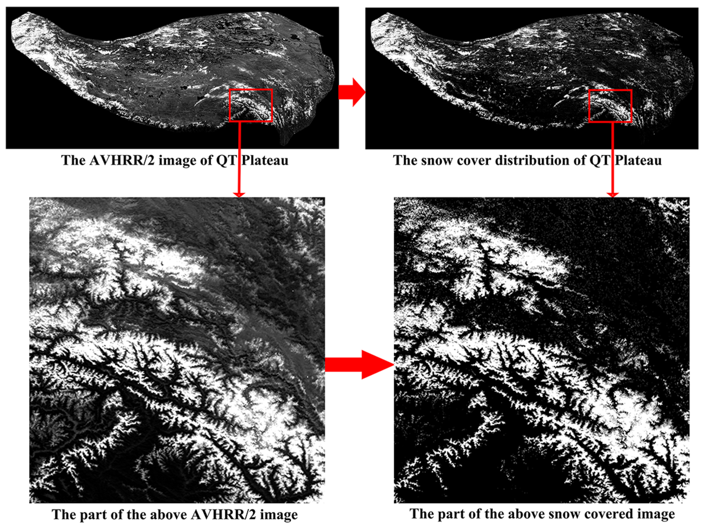
2.1. Study Area and Satellite Data

2.1.1. Study Area

The study area is the Qinghai–Tibet Plateau in southwest China, whose latitude and longitude are about 26°N–40°N and 73°E–105°E, respectively, and whose area and altitude are about 3,000,000 km² and 4000–5000 m, respectively. The plateau has abundant snow cover and glaciers all year round, whose meltwaters are the main run-off sources for the upper reaches of many great rivers. Figure 1 shows the location and terrain of the plateau.

2.1.2. Satellite Data

AVHRR/2 sensors were first used on board the satellite of NOAA-7, in 1981. There are a total of five channels; channel 1 and channel 2 are the visible and near-infrared bands, respectively, channel 3 the is middle-infrared band, and channel 4 and channel 5 are both thermal infrared bands. AVHRR/2 data have a spatial resolution of about 1100 m, a high-temporal-resolution, and a time span of more than 40 years. Note that AVHRR/2 sensors do not possess the channel of 1.6μm, which AVHRR/3 and MODIS sensors all have.

In this study, AVHRR/2 daily data were used, obtained from the National Satellite Meteorological Centre of China, stored as LDF files, including header file and channel data, and then both geometrically corrected and geo-located to [19], and calibrated according to NOAA’s calibration coefficients [20]. Their boundaries are about 17°N–41°N, 65°E–106°E.

2.2. Cloud Removal for the AVHRR/2 Images

2.2.1. Cloud Types

Clouds often cover some ground objects, which are not seen in the remotely sensed images, and need to be removed from the remotely sensed images before the images are used. Different types of clouds have different features, thus, each type of cloud may need a respective approach of removal from the remotely sensed images. According to the altitude and form of clouds, clouds can be classified into various types.

• Low clouds

Low clouds are generally under 2500 m of height, and mainly consist of small water droplets, maybe produce precipitation, and include cumulus, cumulonimbus, stratocumulus, stratus, and nimbostratus. In addition, low clouds have a high brightness temperature in the thermal infrared band, while their optical spectral features are diverse [21].

• Medium clouds

Medium clouds are a combination of small water droplets, supercooled water droplets, and ice crystals or snow crystals, and include high stratus and high cumulus. The height of medium cloud bottom is about 2500–5000 m. High stratus often produces rainfall in summer, and snowfall in winter; in addition, high cumulus can bring about precipitation in a plateau region.

• High clouds

High clouds are composed of small ice crystals, and include cirrus, cirrostratus, and cirrocumulus. The height of the high cloud bottom is higher than 5000 m, but lower in a plateau region. High clouds have a low brightness temperature in the thermal infrared band; however, their albedo is not high [21].

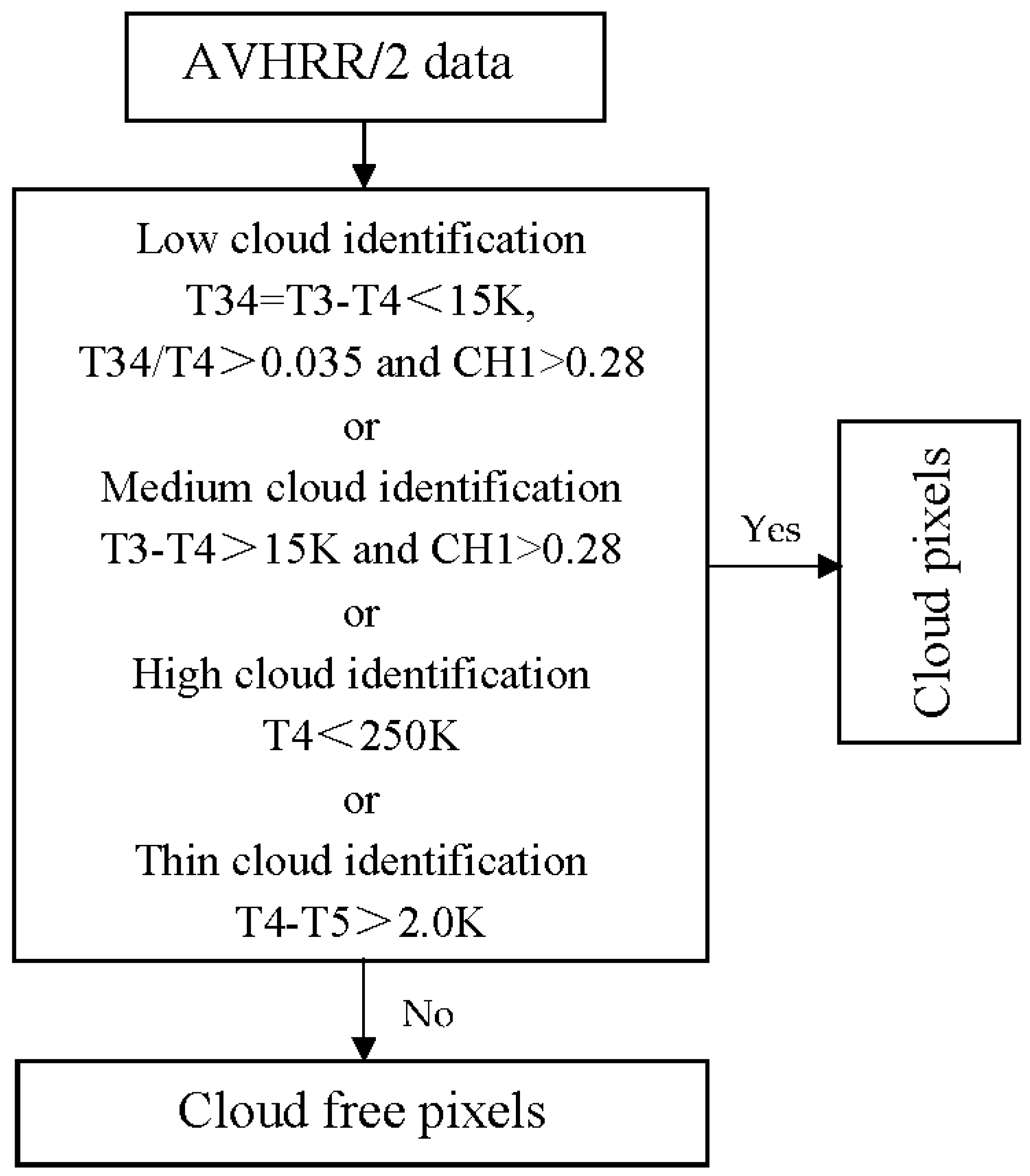
2.2.2. The Identification of Clouds from AVHRR/2 Images

In the remote sensing images including clouds and snow together, it is difficult to remove clouds because the reflectance of clouds and snow is very high in the visible band, especially with regard to AVHRR/2 images, which lack the channel around 1.6μm, and only have two optical channels. It is noted that other ground objects, except snow, are more easily separated from the clouds in the AVHRR/2 images, since the difference in the spectra is quite great between clouds and the other ground objects.

At high elevation, the Qinghai–Tibet Plateau is covered, both permanently and seasonally, with snow, which is of high interest in regard to mapping, but there are often heavy clouds over the plateau. As such, the clouds must be removed from the satellite images, such as from AVHRR/2, to allow for the accurate subpixel snow mapping of the plateau. Undoubtedly, clouds are difficult to remove from images including clouds and snow together. Nevertheless, some methods are proposed for removing clouds from AVHRR/2 images [22,23,24]. These cloud removal methods can be used as the references here.

For fully removing cloud pollution from AVHRR/2 images, clouds are divided into high clouds, medium clouds, low clouds, and thin clouds. Four types of clouds are identified from AVHRR/2 images, and the steps of detecting the four cloud types on the AVHRR/2 images are illustrated in Figure 2.

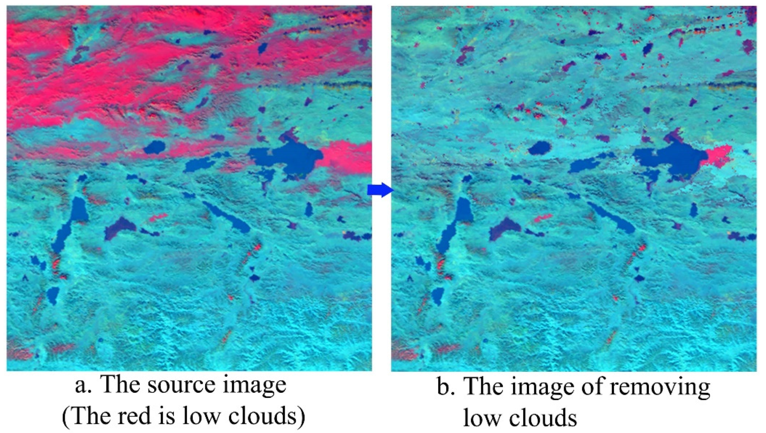
• Identifying low clouds from AVHRR/2 images

Low clouds are low in height, and include supercooled water; thus, their reflectance of about 3.7μm waveband is much higher than that of ice cover on the earth surface [25]. In the Antarctic continent, Turner [23] detected the low clouds based on the data of channel 3. However, Antarctic ground features are quite different to that of the Qinghai–Tibet Plateau; therefore, Turner’s method cannot be used unchanged in the low cloud detection of the plateau.

The detection of the low clouds improves when the data of channel 4 and channel 1 are used in the detection. Based on the experiments using the AVHRR/2 data of 1995, 1998, and 2007, the low cloud detection formula can be obtained as follows:

$$\{\begin{array}{c}\mathrm{T}34=\mathrm{T}3-\mathrm{T}4<15\mathrm{K}\\ \frac{\mathrm{T}34}{\mathrm{T}4}>0.035\\ \mathrm{C}\mathrm{H}1>0.28\end{array}$$

(1)

In Formula (1), T3 and T4 indicate the brightness temperatures of channel 3 and channel 4, respectively, and CH1 and CH2 are the reflectance of channel 1 and channel 2, respectively.

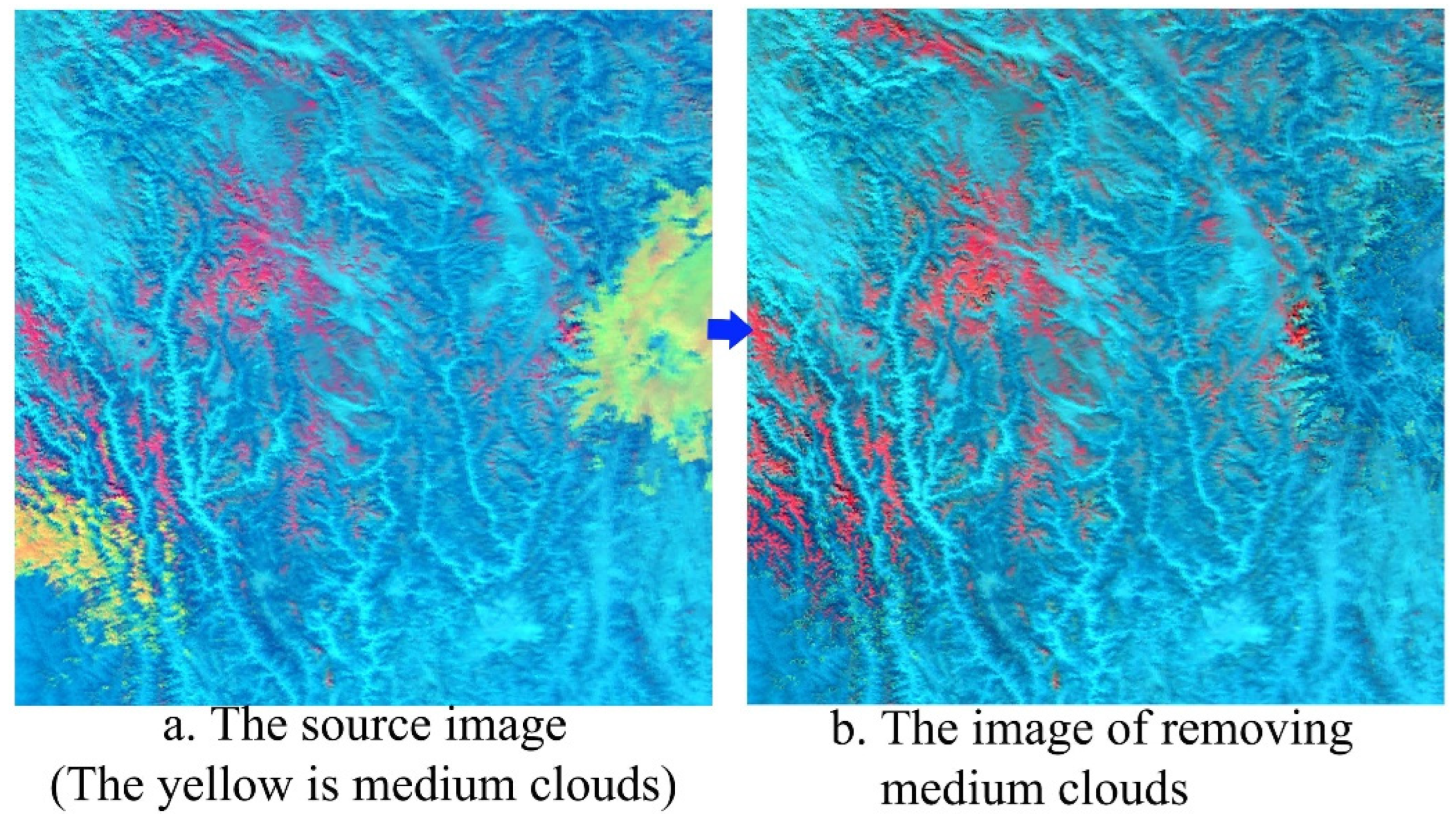
• Identifying medium clouds from AVHRR/2 images

Compared to high clouds and low clouds, the altitude of medium clouds is not too high and not too low, and the reflectance of medium clouds is high. In addition to ice crystals, the medium clouds also include supercooled water, and can be detected using the brightness temperature difference between channel 3 and channel 4. As the data of channel 1 can remove the disturbance of bare land in the detection of the medium clouds, channel 1 is also used in the detection of the medium clouds. Then, based on experiments, the medium-cloud-identifying formula is:

$$\{\begin{array}{c}\mathrm{T}3-\mathrm{T}4>15\mathrm{K}\\ \mathrm{C}\mathrm{H}1>0.28\end{array}$$

(2)

• Identifying high clouds from AVHRR/2 images

The altitude of high clouds is quite high, and little ice crystals are the main component of high clouds; therefore, the ground temperature under high clouds is certainly higher than that of the top of high clouds. In addition, the temperature of ground objects determines the thermal infrared spectra of remotely sensed images; consequently, the high clouds can be separated from ground objects, based on the data of thermal infrared channels in AVHRR/2 images [26].

Here, the channel 4 data are used to detect the high clouds in the AVHRR/2 images over the Qinghai–Tibet Plateau. The threshold of detecting the high clouds is determined to be 250 K, on the basis of the experiments of detecting high clouds. Finally, if the brightness temperature of a pixel is lower than 250 K in channel 4, the pixel is labeled a high cloud pixel.

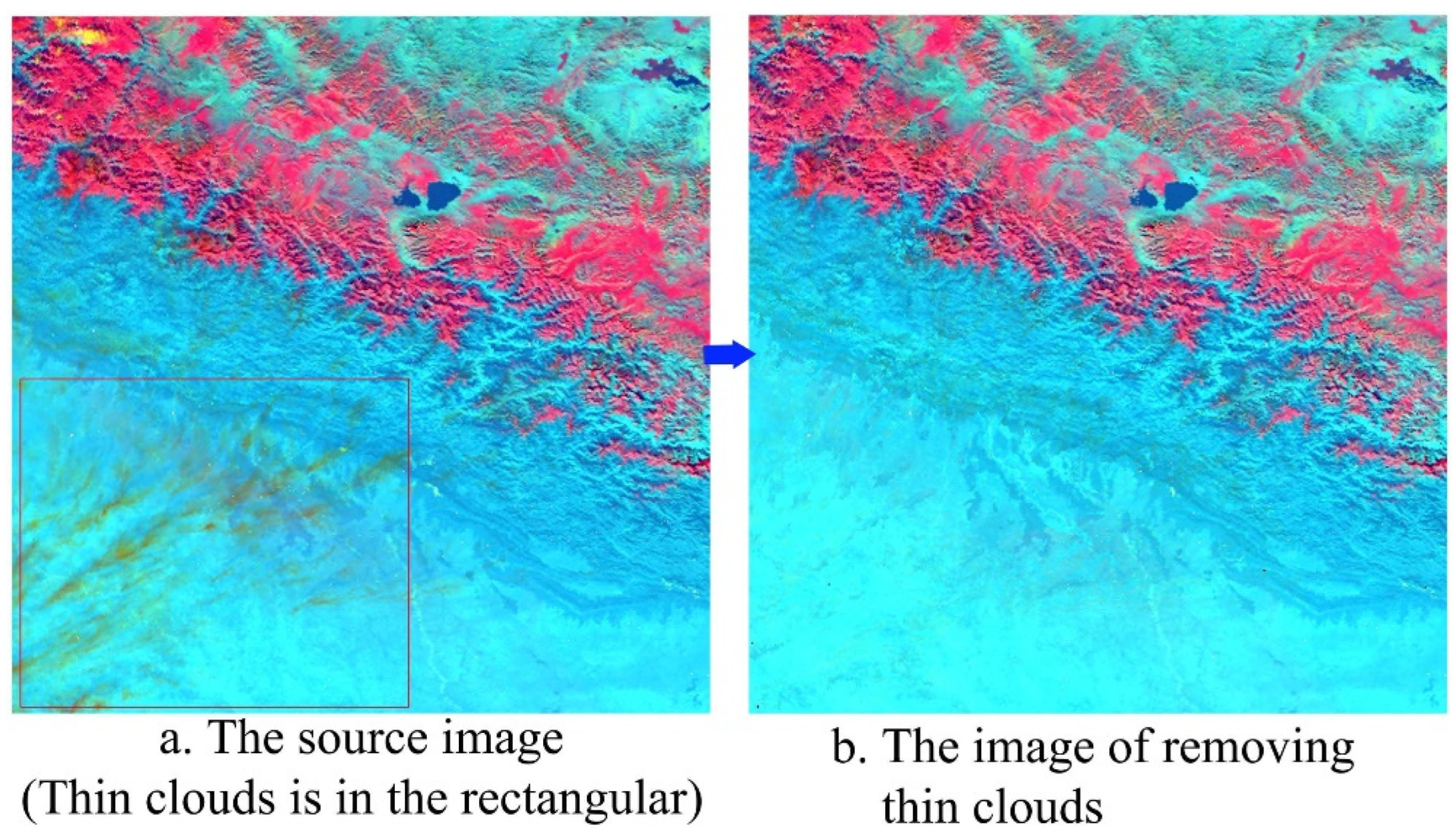
• Identifying thin clouds from AVHRR/2 images

Here, thin clouds are treated as the clouds under which ground objects are hazily seen in AVHRR/2 images; that is, the ground objects cannot be seen clearly, because the surface radiation only partly passes through the thin clouds to sensors, and is partly blocked by the thin clouds. If AVHRR/2 images that do not have the thin clouds removed are used in subpixel snow mapping, then the accuracy is reduced. In this work, the thin clouds are also considered in the cloud removal.

Detecting the thin clouds from AVHRR/2 images using the brightness temperature differences between channel 4 and channel 5 is reported by Yamanouchi in [22]. Here, Yamanouchi’s method is used for removing the thin clouds. Thin clouds have a difference in the brightness temperature between channels 4 and 5 [22]. The experiments indicate that the brightness temperature differences of the thin cloud pixels are larger than 2 K, namely, the pixels are determined as thin cloud pixels if T4–T5 > 2.0 K.

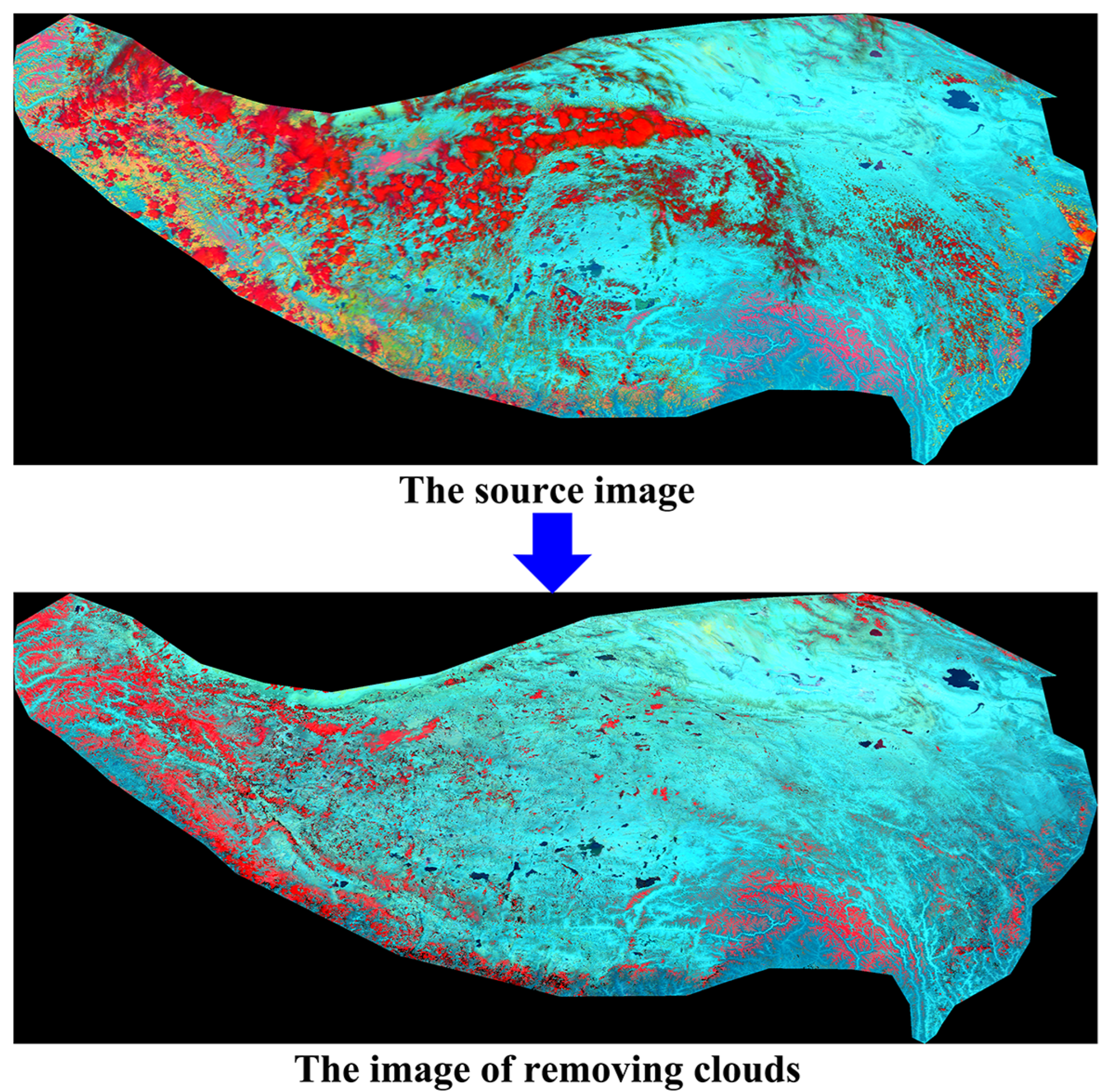
2.2.3. The Substitution of Cloud Pixels in the AVHRR/2 Images

The removal of clouds from AVHRR/2 images includes two steps: the detection of cloud pixels, and the substitution of cloud pixels. According to the above results of cloud detection, every cloud pixel in an AVHRR/2 image is substituted with a cloud-free pixel of the same position in another AVHRR/2 image that was taken temporally nearest to the substituted AVHRR/2 image. However, the temporal difference of the two images is not generally more than a certain time length, such as 7 or 10 days. It is likely that the time length of more than 7 or 10 days is better for cloud removal; however, too long a time length can result in changes in surface features.

2.2.4. Contrasting Cloud Removed Images with Their Source Images

After the cloud pollution is removed from the AVHRR/2 images, the clouds do not disturb subpixel snow mapping; therefore the subpixel snow mapping is reliable. In addition, while the cloud pollution was removed from the AVHRR/2 images here, the snow cover remained in the AVHRR/2 images. This is indicated in Figure 3, Figure 4, Figure 5, Figure 6 and Figure 7, which compare figures between the images with the clouds removed and their source images. In fact, a lot of images were used to validate the algorithm of cloud removal, and it turns out that the cloud removal algorithm is reliable and feasible.

However, the results of cloud removal are not validated quantitatively, because, at present, reference data are difficult to find. A great many experimental results of cloud removal indicate, to some degree, that the algorithm of cloud removal is reliable, and the final results of subpixel snow mapping also prove indirectly that the algorithm of cloud removal in this research is reliable. In addition, further explanation is needed, as the mechanism of detecting clouds is not studied in deep here, and the method of detecting clouds may only be suitable for use in the Qinghai–Tibet Plateau. However, there also are some other successful cloud removal methods, such as the cubic spline interpolation algorithm in [14,27].

2.3. Subpixel Snow Mapping Using Daily AVHRR/2 Data

In this work, the subpixel snow mapping of the Qinghai–Tibet Plateau included two parts: firstly, the removal of cloud, and then the subpixel snow mapping itself. After removing clouds from the AVHRR/2 images, the subpixel snow mapping was implemented; the progress steps are shown Figure 8. In the subpixel snow mapping, a linear spectral mixture model was used to unmix the mixed pixels of a remotely sensed image. The end-members were selected automatically and directly from the AVHRR/2 image used, using the normalized difference vegetation index (NDVI), and channels 1 and 2 of the AVHRR/2 image. The end-members are different from each other for different AVHRR/2 images. However, with a view to reduce the computing complexity of pixel unmixing, only two kinds of end-members were used simultaneously to perform the spectral mixture computation of a mixed pixel.

2.3.1. Linear Spectral Mixture Model

Among the spectral mixture analysis models of remotely sensed images, linear spectral mixture model is robust, easy to use, and the most widely used; thus, it is used in this work.

Supposing that each column of a matrix M represents the end-member spectra of one ground object class, x is the spectra of each band of a pixel, f is the areal percent of each end-member within a mixed pixel, and e is the observational error. Therefore, a linear spectral mixture model of a mixed pixel can be expressed as:

$$\mathrm{X}=\mathrm{Mf}+\mathrm{e}$$

(3)

2.3.2. Approach to Selecting Multiple Snow and Non-Snow End-Members

In remotely sensed images, the same class of ground objects may have different spectra. Therefore, if one class of ground objects only use one kind of end-member spectrum in the unmixing computation of mixed pixels, some additional errors are introduced into the results of the unmixing. For improving the precision of the subpixel snow mapping, multiple end-members were extracted for one class of ground objects in the unmixing computation of this work.

• Extraction of snow end-members from AVHRR/2 data

Snow is comprised of ice crystals, liquid water, and air, and has a very high reflectance in the visible band. In the band of 0.4 μm–0.6 μm, snow has a very strong reflection height, and its reflectance is close to 100%. Although the reflectance of snow is very high in the visible and near-infrared bands, its reflectance is lower with an increase in wavelength, and its reflectance is lowest in the short-wave infrared band of almost 1.6 μm.

Channel 1 and channel 2 of the AVHRR/2 data are a visible band and a near-infrared band, respectively, and the snow reflectance of the two channels is quite high, however, the snow reflectance of channel 1 is generally higher than that of channel 2. The normalized difference vegetation index (NDVI) is reliable and useful in the indication of land surface features, and its computational formula is:

$$\mathrm{NDVI}=\left(\mathrm{CH}2-\mathrm{CH}1\right)/\left(\mathrm{CH}2+\mathrm{CH}1\right)$$

(4)

where CH1 and CH2 are the reflectance of channel 1 and channel 2 of the AVHRR/2 data, respectively. As the snow reflectance of channel 2 is lower than that of channel 1, the NDVI of snow should be small numerical values; according to Formula (4), the NDVI of pure snow should be below 0, and the NDVIs of mixed snow pixels should be near to 0. Therefore, a rule for selecting pure snow pixels can be assumed as:

NDVI < 0

(5)

Certainly, it is not enough if only the NDVI is used for selecting pure snow pixels, because the errors may appear in selection of pure snow pixels.

Since the snow reflectance of channel 1 is very high, channel 1 can be used to select pure snow pixels, that is:

CH1 > m

(6)

where m is a threshold. Many pure snow pixels were extracted from different remotely sensed data, including AVHRR data, MODIS data, and TM data, and it is found that the snow pixels whose reflectance is greater than 0.8 are pure snow pixels; consequently, the reflectance of channel 1 must be greater than 0.8.

Therefore, the rules for selecting pure snow pixels can be determined as:

$$\{\begin{array}{c}\mathrm{N}\mathrm{D}\mathrm{V}\mathrm{I}<0\\ \mathrm{C}\mathrm{H}1>0.8\end{array}$$

(7)

Finally, the experiments also prove that Formula (7) is reliable.

• Extraction of non-snow end-members from AVHRR/2 data

Besides having snow cover, the Qinghai–Tibet Plateau is mainly covered with bare land, vegetation, and water. No matter the season, the bare land covers most of the plateau. Therefore, the pure pixels of the bare land should be selected as a class of non-snow end-members. There is little vegetation on the plateau in winter, but much in summer, consequently, the pure pixels of vegetation should be also selected as a class of non-snow end-members. Although the area of water is small in the plateau, it cannot be ignored. Here, the pure pixels of water should also serve as a class of non-snow end-members. In this work, the end-members of non-snow include three classes of ground objects, namely, bare land, vegetation, and water.

• Rules for extracting the end-members of bare land

The bare land reflectance of channel 1 is between 10% and 20%, and the reflectance of channel 2 is mainly between 20% and 25% (Figure 9). The bare land reflectance of channel 2 is greater than that of channel 1, however, the reflectance difference between them is not big, thus, the NDVIs of bare land are also small, generally from 0 to 0.2.

In the experiments, the reflectance differences of channel 2 and channel 1 are useful for extracting the end-members of bare land. It is found that the reflectance differences are less than 0.1, according to Figure 9.

In addition, the reflectance of channel 1 is also used for extracting end-members of bare land, in order to improve the reliability of the end-members here.

Finally, the rules for extracting the end-members of bare land are as follows:

$$\{\begin{array}{c}0 < \mathrm{NDVI} < 0.2\\ \mathrm{CH}2 - \mathrm{CH}1 < 0.1\\ \mathrm{CH}1 < 0.28\end{array}$$

(8)

2.

Rules for extracting the end-members of vegetation

The spectra of vegetation are deeply influenced by chlorophyll. The reflection height and absorption valley are in the visible waveband, and the middle wavelengths are about 0.55 μm and 0.67 μm, respectively. In the near-infrared band, the reflectance of vegetation is very high, and its height generally appears at about 1.1 μm.

As vegetation has such spectral features, especially the reflectance of channel 2, which is much higher than that of channel 1, the NDVI of vegetation is very high. In fact, the NDVI of vegetation is highest in all the ground objects of the Qinghai–Tibet Plateau; therefore, the end-members of vegetation can be obtained from the AVHRR/2 images using NDVI. NDVI values are low in the regions where vegetation is sparse. Here, it can be found that the NDVI values of vegetation are more than 0.3, as shown in Figure 10. Therefore, the NDVI threshold for extracting the end-members of vegetation is about 0.3, and this is proven by experiments. Therefore, the rule for extracting the end-members of vegetation is:

NDVI > 0.3

(9)

3.

Rules for extracting the end-members of water

In AVHRR/2 data, the water reflectance of channel 1 is about 2 times that of channel 2, and the visible and near-infrared reflectance of water is very low (as in Figure 11).

In addition, the NDVI of water is certainly smaller than 0. Therefore, the rules for extracting water can be as follows:

$$\{\begin{array}{c}\mathrm{N}\mathrm{D}\mathrm{V}\mathrm{I}<0.0\\ \frac{\mathrm{CH}1}{\mathrm{CH}2}>2.0\end{array}$$

(10)

If only Formula (10) is used to extract pure pixels of water from AVHRR/2 images, some errors may appear in the extraction. Generally, the reflectance of water is very low, compared with other ground objects. Thus, channel 1 can be used for improving the accuracy of the extraction. In the experiments of the extraction, after CH1 < 0.05 was used, its accuracy improved greatly. Finally, the rules for extracting the end-members of water are:

$$\{\begin{array}{c}\mathrm{N}\mathrm{D}\mathrm{V}\mathrm{I}<0.0\\ \frac{\mathrm{CH}1}{\mathrm{CH}2}>2.0\\ \mathrm{C}\mathrm{H}1<0.05\end{array}$$

(11)

2.3.3. The Unmixing of Mixed Pixels in AVHRR/2 Images

After the spectral mixture model and the approaches of selecting the end-members are determined, the mixed pixels can be unmixed for obtaining their snow area percentage. In the following, the unmixing procedure of AVHRR/2 images is described.

• Selection of snow end-members and non-snow end-members according to the above rules of extracting end-members

Following the above rules, the snow and non-snow end-members can be extracted from each AVHRR/2 image, respectively. The obtained snow and non-snow end-members are stored in their respective databases, namely, the snow end-member database and non-snow end-member database. At the same time, the position information of each snow or non-snow end-member is also saved in the respective databases. In addition, each AVHRR/2 image has also its own end-member database, which are different from those of other AVHRR/2 images.

• Approaches to using snow and non-snow end-members in the unmixing of mixed pixels in AVHRR/2 images

If all end-members in a database are used in the unmixing calculation, the calculation cost is very large. To reduce the calculation cost, the end-members of one class are divided into different subgroups, according to the end-member features of the class, and the unmixing calculation only uses the spectral mean value of the end-members in each subgroup. The spectral mean value is also defined as the typical spectral value of the subgroup (i.e., a typical end-member). The end-members of a same subgroup are more similar in their spectral features than those of other subgroups, thus, the typical end-member represents its own subgroup in the spectral feature. If the typical end-members are used in the unmixing computation, instead of all the end-members in the subgroup, the number of end-members used in the unmixing calculation is greatly reduced, as is the calculation cost, and the unmixing speed increases.

Each scene of an AVHRR/2 image covers a large area, and the ground objects of the same class in different regions generally have different spectral features. Consequently, the various ground objects of one class in the same region should have more similar spectral features than those of the class in different regions. If a mixed pixel is adjacent to a pure pixel as an end-member, it is called the neighboring end-member of the mixed pixel. In this work, the spatial distance between a mixed pixel and its neighboring end-member cannot be greater than 5 pixels. Generally speaking, the neighboring end-members are more reliable in the unmixing calculation than the typical end-members [8].

Before unmixing a mixed pixel, its neighborhood must be searched to find its neighboring pure pixels (i.e., neighboring end-members) in the AVHRR/2 image used. After its neighboring end-members are found, all neighboring and typical end-members are used in the unmixing calculation. In addition, the unmixing calculation should be based on the linear spectral mixture model. However, only the best result is needed in the unmixing calculation. The best result can be obtained using typical end-members and/or neighboring end-members. Of course, if there are no neighboring end-members, typical end-members will be used alone in the unmixing. Then, the snow area percentage of the mixed pixel can be also obtained through the unmixing calculation. In this way, the subpixel snow mapping is faster and more reliable than processes not using these approaches.

2.3.4. Subpixel Snow Mapping through a Look-Up Table

According to the unmixing algorithm above, a computer code can be written out for calculating the snow area percentage of a mixed pixel in AVHRR/2 images. Then, the subpixel snow distribution of the Qinghai–Tibet Plateau can be also obtained. But a great amount of time is needed for the calculation of the subpixel snow mapping, and its calculating speed is also very slow. Therefore, it is necessary to find an approach to speed up the subpixel snow mapping.

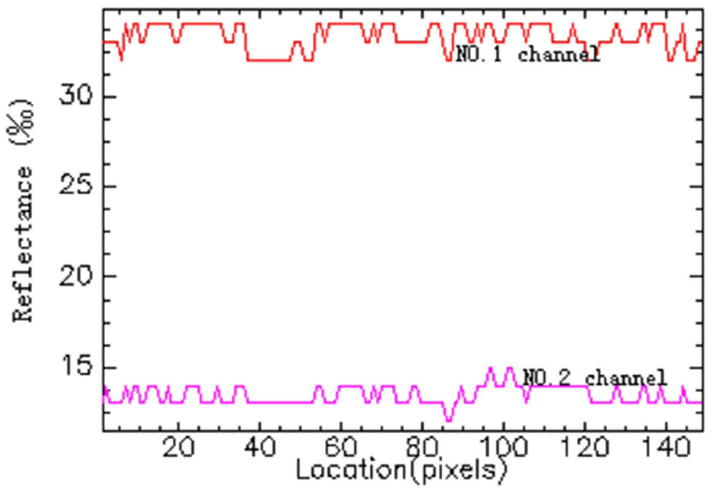
• Look-up table and sample spectra

For speeding up the subpixel snow mapping, and reducing the calculation time, a look-up table comparing sample spectra of mixed pixels and their own snow area percentage was introduced into the subpixel snow mapping here. The sample spectra are explained in the following. By comparing the spectrum of a certain mixed pixel with a sample spectrum, its snow area percentage can be found in the look-up table.

Here, sample pixels are the pixels that represent other pixels in their spectra, that is, the spectra of sample pixels are similar to those of the represented pixels in an AVHRR/2 image. In addition, the spectra of sample pixels are also called the sample spectra in the paper. The sample spectra are unmixed, according to the algorithm of spectral mixture above, and the snow area percentage of the sample pixel can be obtained. After all sample pixels are unmixed, the look-up table between sample spectra and their own snow area percentage can be established for the AVHRR/2 image.

• Approach to selecting the sample spectra from AVHRR/2 images

Whether or not all the sample spectra really represent all the mixed pixel spectra of a certain AVHRR/2 image directly determines the accuracy of the subpixel snow mapping. The selection of sample pixels is very important for the subpixel snow mapping of AVHRR/2 data. The method of selecting sample pixels is described in the following (shown in Figure 12):

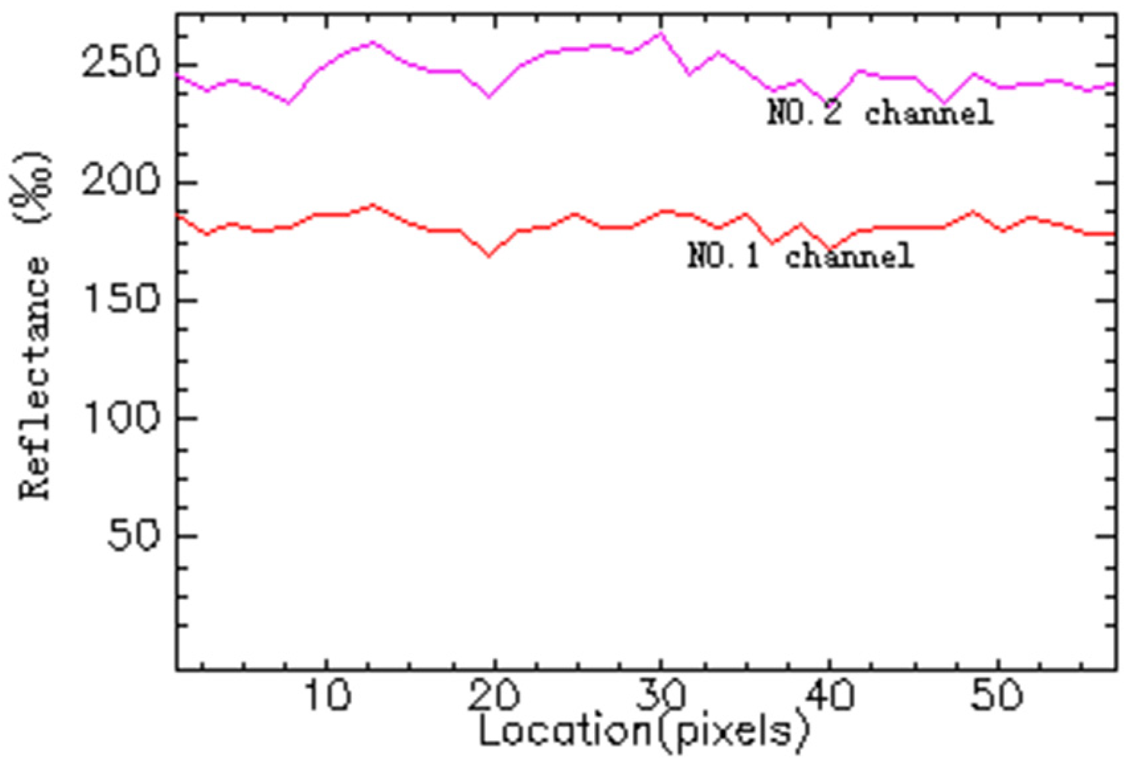
• For an AVHRR/2 image, the reflectance of all its mixed pixels are multiplied by 1000, then the values of reflectance are changed into integers, from 0 to 1000;
• According to the reflectance integral values of channel 1, the mixed pixels of the same reflectance value constitute one pixel group; that is, all the mixed pixels are divided into 1001 pixel groups because the reflectance has 1001 kinds of integral values in total;
• According to the reflectance value distribution of channel 2, each pixel group is also divided into several pixel subgroups. In one pixel group, if there are some pixel clusters with close channel 2 reflectance values, each pixel cluster serves as a subgroup. Then, from each pixel subgroup, one pixel, which best represents all the pixels of the subgroup, is selected as the sample pixel of that subgroup, and its spectrum is also the sample spectrum. Generally, the pixel is the spectral mean value of the subgroup.

• How to use the look-up table

After the look-up table of an AVHRR/2 image is established, the subpixel snow mapping of the image can be implemented. In the subpixel snow mapping, each mixed pixel of the image is compared to every sample pixel of the look-up table, and the most similar sample spectra of the mixed pixel are found. The snow area percentage is equal to that of the most similar sample pixel. If the most similar sample pixel of each mixed pixel is found, the snow area percentages of all the mixed pixels are also obtained for the AVHRR/2 image.

Here, the rules of determining the most similar sample spectra of a mixed pixel are:

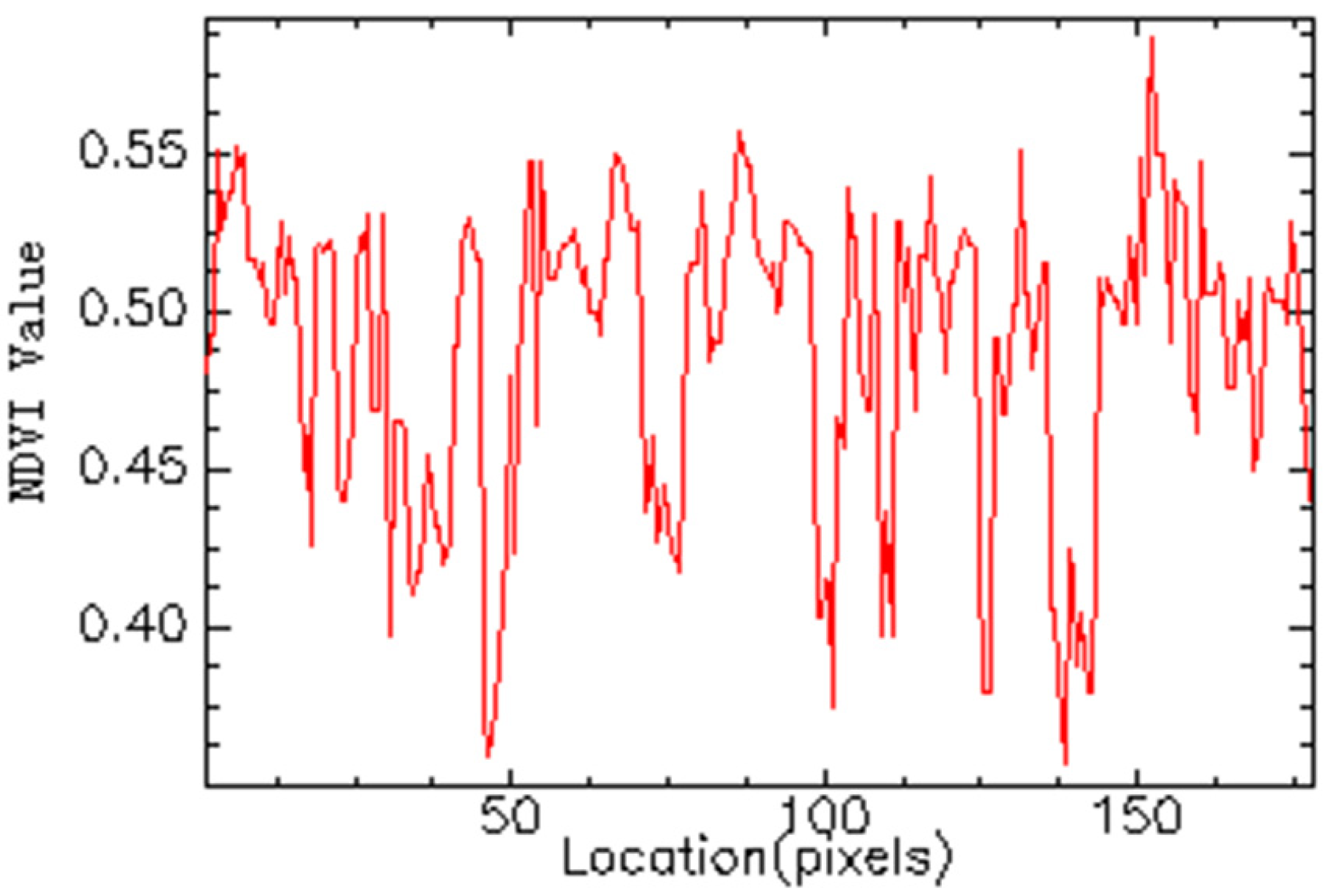
• The difference sum between the NDVI values, and band 1 and band 2 reflectance values of the mixed pixel and its most similar sample pixel is the smallest among all the difference sums between the mixed pixel and sample pixels;
• The respective differences between the NDVI values, and band 1 and band 2 reflectance values of the mixed pixel and its most similar sample pixel are not greater than their difference sum. For example, the difference between NDVI values, as well as band 1 or band 2 reflectance values, must be less than the difference sum of the three kinds of data between the mixed pixel and its most similar sample pixel.

Lastly, the snow end-members and non-snow end-members are added to the unmixing results of the mixed pixels, and the final results of the subpixel snow mapping can be obtained for the AVHRR/2 image. The snow-covered area of the AVHRR/2 image includes the fractional snow cover of the mixed pixels, snow end-members, and non-snow end-members. Of course, the snow area percent of a snow end-member is 1, and is 0 for a non-snow end-member.

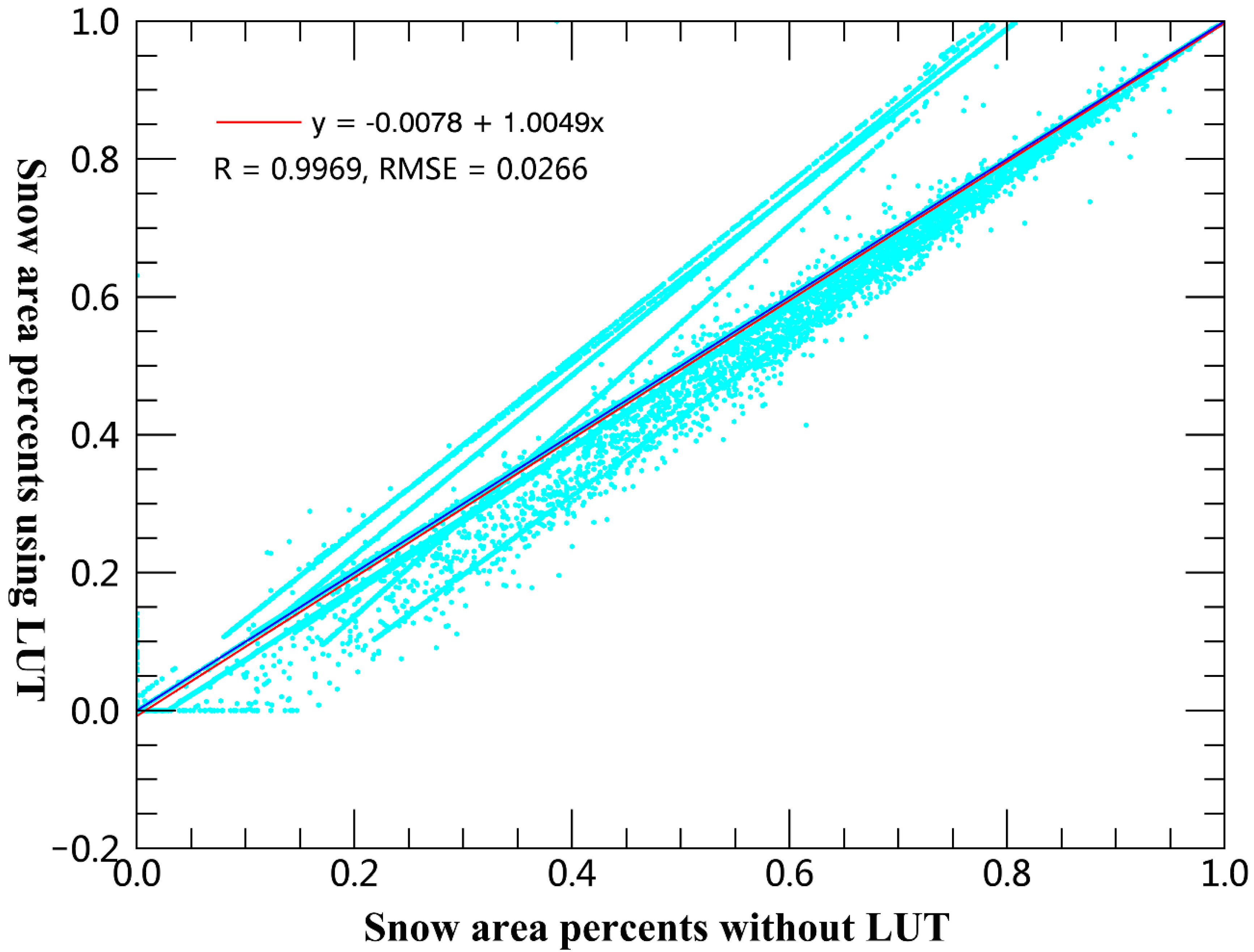
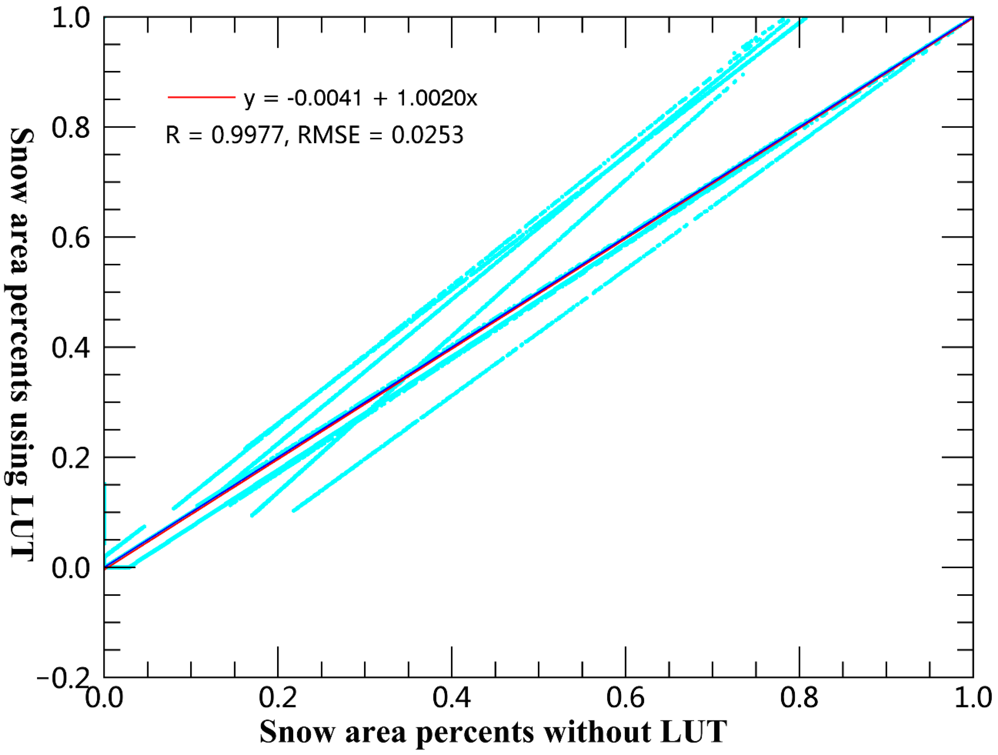
• Comparison between the subpixel snow mappings using the look-up table and without using the look-up table

Based on the same AVHRR/2 image, subpixel snow mapping was performed using the look-up table, and without using the look-up table, and the two results of snow mapping were compared with each other, in order to test the reliability and feasibility of the subpixel snow mapping using the look-up table (Figure 13 and Figure 14).

In Figure 13 and Figure 14, the two results of snow mapping are quite consistent, their correlation coefficients are 0.9969 and 0.9980, respectively, and their RMS errors are 0.0264 and 0.0245, respectively. That indicates that using the look-up table is feasible and reliable in the subpixel snow mapping.

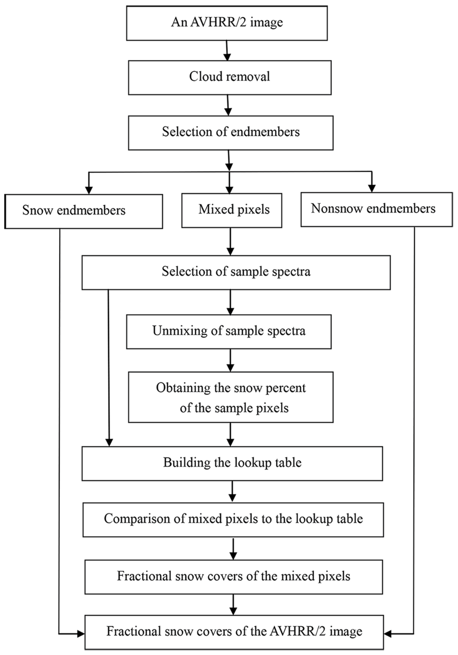
2.3.5. Steps of the Subpixel Snow Mapping of Qinghai–Tibet Plateau Using Daily AVHRR/2 Data

As described above, the algorithm of the subpixel snow mapping using daily AVHRR/2 data over the Qinghai–Tibet Plateau was established. In the following, the steps of the subpixel snow mapping are described briefly (shown in Figure 8):

• According to the above algorithm of cloud removal, the cloud-removed AVHRR/2 data are obtained. In the research, the clouds must be removed from the AVHRR/2 data first, before the AVHRR/2 data are used in the subpixel snow mapping;
• According to the above approach of end-member selection, all the pixels of a certain AVHRR/2 image are divided into three classes, i.e., snow end-members, non-snow end-members, and mixed pixels;
• Using the unmixing calculation, the snow area percentage of the mixed pixels is obtained. In addition, the pure pixels serving as snow and non-snow end-members are added directly to the results of the subpixel snow mapping, and do not join the unmixing calculation. The unmixing process of the mixed pixels is as follows:
  • According to the above selection approach of sample spectra, sample pixels are selected from the AVHRR/2 image, and the sample spectra obtained;
  • The sample spectra are unmixed using the above algorithm of spectral mixture, and the snow area percent of sample spectra obtained. Then, a look-up table of the sample spectra and their own snow area percentage can be established;
  • Each mixed pixel of the AVHRR/2 image is compared to all the sample pixels in the look-up table. The snow area percentage is equal to that of the sample pixel with the most similar spectrum;

• The fractional snow cover of the mixed pixels, plus those of snow end-members and non-snow end-members, is the final result of the subpixel snow mapping. Thus, the snow-covered area of the AVHRR/2 image includes fractional snow covers of the mixed pixels and snow end-members.

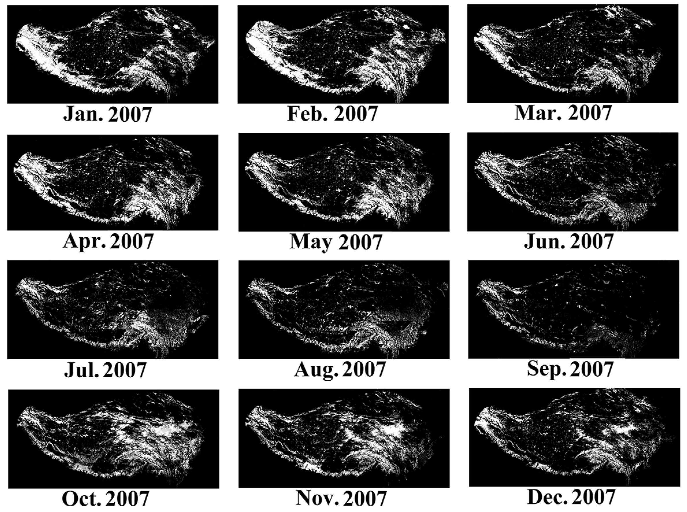
In addition, after the look-up table is used, the calculating time of the subpixel snow mapping is only 1/3 of the time compared to when the look-up table is not used, according to corresponding experiments. The look-up table largely improves the running speed of the subpixel snow mapping using AVHRR/2 data.

3. Results

3.1. Validation of the Subpixel Snow Mapping

3.1.1. Thematic Mapper (TM) Data and Their Processing

Here, TM data are used to validate the subpixel snow mapping using daily AVHRR/2 data of the Qinghai–Tibet Plateau, and have seven wave bands. Among the seven bands, band 1 to band 5 and band 7 are visible and near-infrared bands, and their spatial resolution is 30 m. The central wavelengths of the six bands are 0.49, 0.56, 0.66, 0.83, 1.67, and 2.22 μm, respectively.

The pixel values of TM data are recorded with digital numbers (DN). For extracting snow pixels from the TM images, the DN values of pixels need to be converted into the reflectance of the pixels. However, the conversion is not described in detail here.

3.1.2. The Extraction of Snow Cover from the TM Data

The reflectance of snow is high in the visible band of 0.4 μm–0.7 μm, but low in the near infrared band of 1.55 μm–1.75 μm, which is very different from other ground objects. Band 2 (0.52 μm–0.60 μm) of the TM data belong to the visible band, and band 5 of the TM data is exactly the near-infrared band of 1.55 μm–1.75 μm. According to the reflectance features of snow, snow pixels can be identified from TM images.

Generally, the normalized difference snow index (NDSI) is useful for identifying the snow pixels of remotely sensed images, and can be obtained with band 2 and band 5, as follow [28]:

$$\mathrm{NDSI}=\frac{\left(\mathrm{TM}2-\mathrm{TM}5\right)}{\left(\mathrm{TM}2+\mathrm{TM}5\right)}$$

(12)

In Formula (14), TM2 and TM5 are the reflectance of band 2 and band 5 of the TM data, respectively. However, because the visible reflectance of water is also higher than that of its near-infrared, water pixels may be confused with snow pixels in a binary snow classification, if the NDSI serves as the only criterion of classification.

The water strongly absorbs the radiation of near-infrared, but the snow only weakly absorbs it, so the reflectance of band 4 is used to identified snow pixels of the TM images.

It should also be possible to obtain the models of snow extracted from the TM images; however, is not described in detail here because this is a common issue. In the end, the models of binary snow classification for the TM data are:

$$\{\begin{array}{c}\mathrm{N}\mathrm{D}\mathrm{S}\mathrm{I}>0.4\\ \mathrm{T}\mathrm{M}4>0.11\end{array}$$

(13)

where TM4 is the band 4 reflectance of TM data.

According to the above models, the snow pixels can be extracted from the TM images, and the snow-covered areas of the TM images can be obtained.

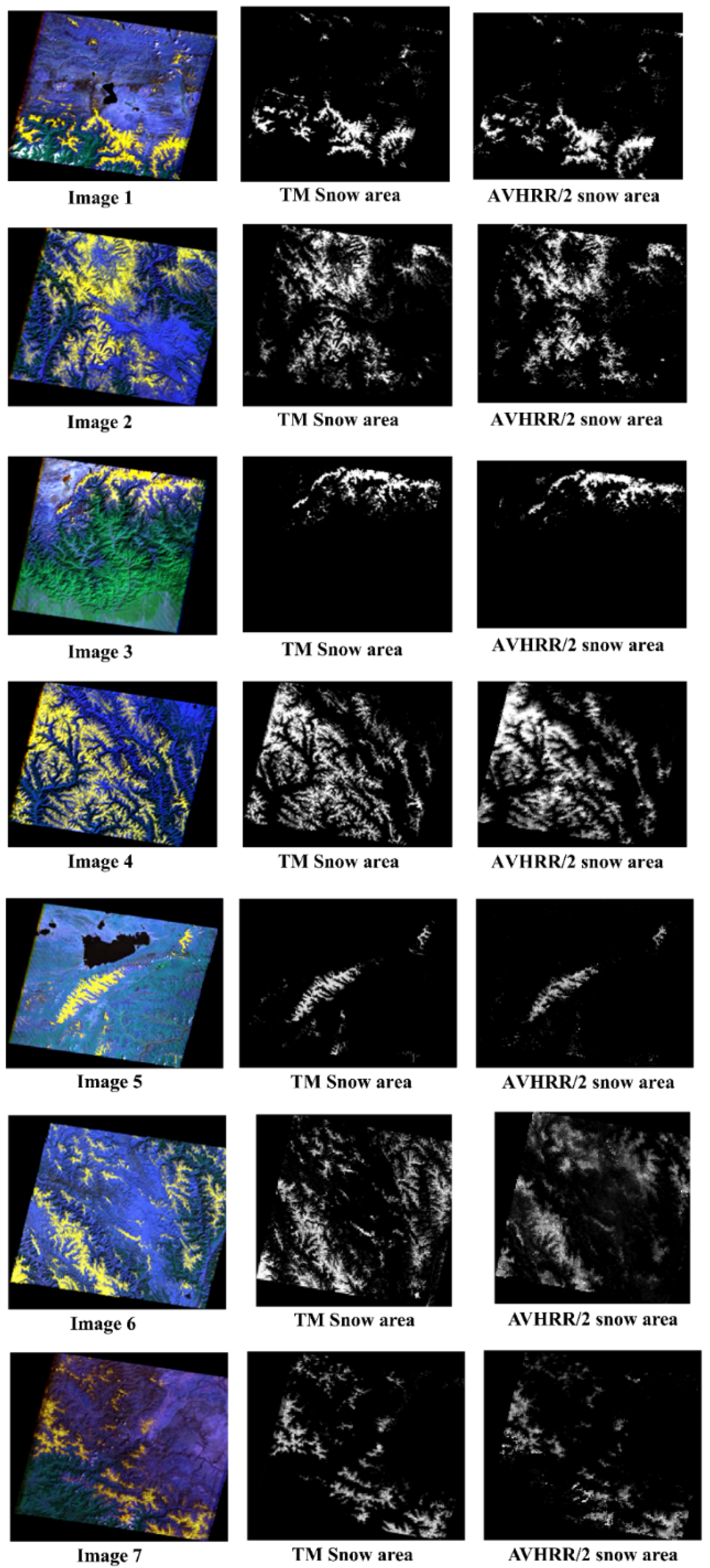
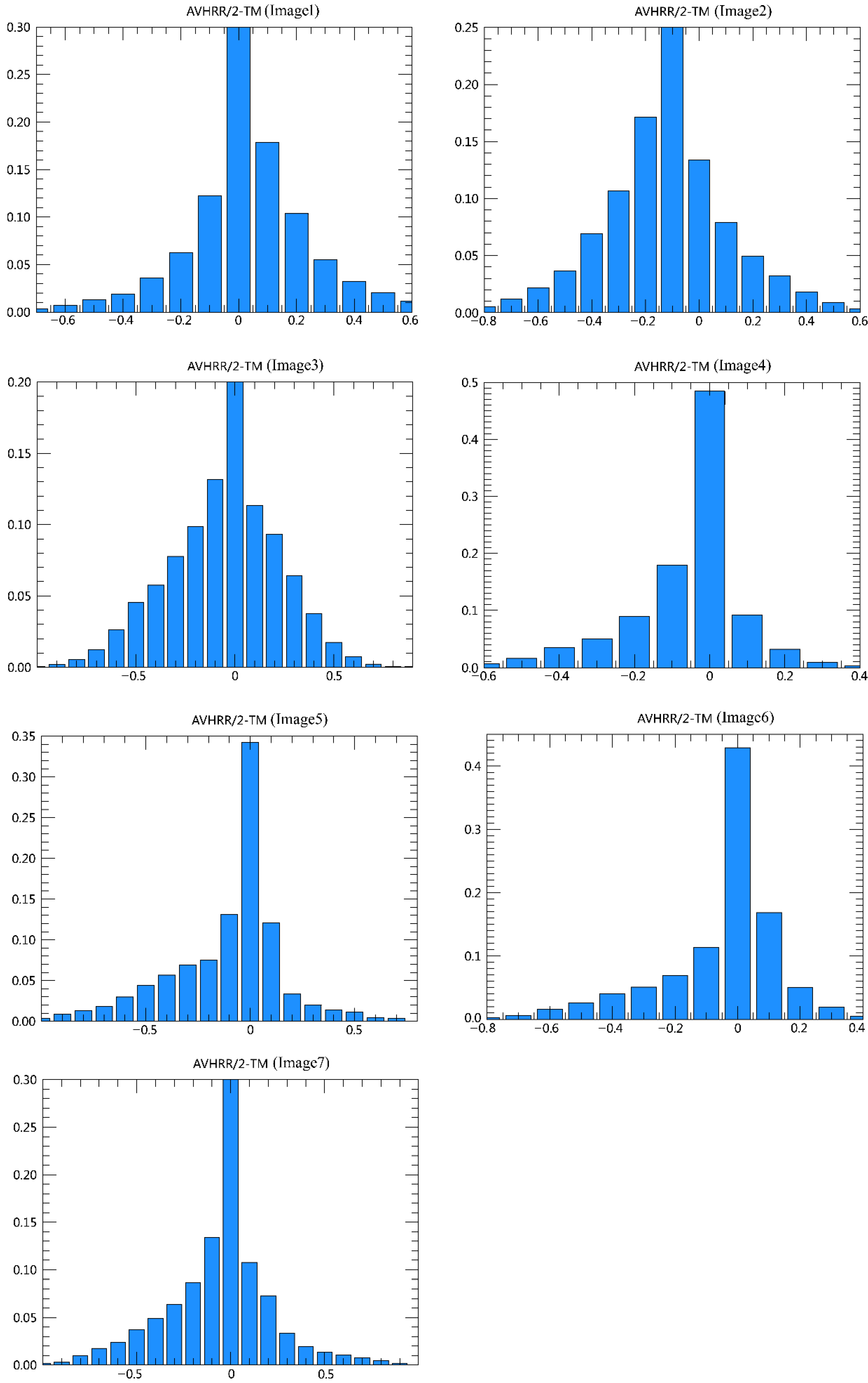
3.1.3. Validation of the Subpixel Snow Mapping

The snow cover image of binary snow classification from the TM data is resampled to the same spatial resolution as the AVHRR/2 data, and then the fractional snow cover data from the TM data are obtained, with resolutions identical to that of the AVHRR/2 data. In addition, the fractional snow cover data from TM data and AVHRR/2 data are rectified into the same projection system. By means of comparison between the fractional snow cover data from the TM data and AVHRR/2 data, the accuracy and precision of the subpixel snow mapping from AVHRR/2 data is confirmed.

3.2. The Results of Comparing to the TM Data

Here, seven scenes of TM images over the Qinghai–Tibet Plateau (Figure 15) are selected, and used to test the subpixel snow mapping. The spatial ranges of the seven TM images are described in

Table 1. The parameters of the 7 TM images.

Image	Latitude	Longitude	Orbit	Row	Date
Image 1	27°53′49.88″N 29°49′54.75″N	84°28′23.30″E 86°56′34.61″E	141	40	6 October 2006
Image 2	29°19′14.67″N 31°15′14.35″N	98°36′48.02″E 101°8′8.07″E	132	39	2 December 2006
Image 3	26°27′26.18″N 28°23′26.99″N	88°39′26.81″E 91°5′18.76″E	133	40	23 December 2007
Image 4	27°56′42.85″N 29°49′13.34″N	96°39′25.17″E 99°18′2.60″E	138	41	25 December 2006
Image 5	29°21′16.25″N 31°15′52.25″N	89°22′43.10″E 91°50′19.10″E	138	39	1 August 2017
Image 6	29°24′36″N 31°12′0″N	97°8′42″E 99°13′30″E	133	39	16 November 1992
Image 7	30°46′30.19″N 32°42′54.19″N	77°22′30.06″E 79°36′18.06″E	146	38	23 September 2016

.

For reducing the error of snow mapping from the geometric correction and varying spatial resolutions of the pixels in an AVHRR image, in this work the pixels of the validated data are resampled into four kinds of grids during the validation of the subpixel snow mapping, such as 1100 × 1100 m, 2200 × 2200 m, 4400 × 4400 m, and 8800 × 8800 m. The validation of the subpixel snow mapping is implemented according to the four classes of grid scales. At the edge of the swath, the spatial resolution is much coarser than in nadir, so the larger of the grids are more reliable for validating the pixels at the edge of the swath. With increasing grid scales, the error from the coarser resolutions at the edge and geometric correction should become smaller, and the accuracies of the validation higher (shown in

Table 2. The validation results of the subpixel snow mapping in this work.

Image	Resolution (m)	R	R2	RMSE
1	1100	0.8760	0.76738	0.0750
	2200	0.9136	0.83466	0.0610
	4400	0.9582	0.89208	0.0380
	8800	0.9759	0.9182	0.0262
	8800	0.9759	0.91815	0.0262
2	1100	0.8555	0.73188	0.0810
	2200	0.8898	0.79174	0.0707
	4400	0.9445	0.89208	0.0497
	8800	0.9642	0.9297	0.0402
	8800	0.9642	0.92968	0.0402
3	1100	0.8461	0.71588	0.1170
	2200	0.8802	0.77475	0.1000
	4400	0.9446	0.89226	0.0663
	8800	0.9725	0.9458	0.0466
	8800	0.9725	0.94576	0.0466
4	1100	0.9067	0.82210	0.0492
	2200	0.9389	0.88153	0.0420
	4400	0.9723	0.94537	0.0305
	8800	0.9802	0.96079	0.0229
5	1100	0.8332	0.6942	0.0703
	2200	0.8554	0.7317	0.0691
	4400	0.9404	0.8843	0.0517
	8800	0.9732	0.9471	0.0427
6	1100	0.8507	0.72369	0.1104
	2200	0.8563	0.73325	0.1087
	4400	0.8825	0.77881	0.1006
	8800	0.9172	0.84126	0.0902
7	1100	0.8018	0.64288	0.1030
	2200	0.8120	0.65934	0.1017
	4400	0.8222	0.67601	0.0827
	8800	0.8635	0.74563	0.0647

Note: R indicates correlation coefficient.

).

4. Discussion

Following the above methods, the results of subpixel snow mapping are obtained and validated. Figure 15 shows the comparisons between the snow area distributions from the TM data and AVHRR/2 data. Based on Figure 15, it is found that the snow area distributions from the AVHRR/2 data are very similar to those from the TM data. To a certain degree, this shows that the algorithm of the subpixel snow mapping in this work is reliable.

To better validate the accuracy and reliability of the subpixel snow mapping, linear regression between the snow-covered areas of AVHRR/2 data and the respective TM data is performed, and the results of the linear regressions are given in Table 2. For the grid scales of 1100 × 1100 m, 2200 × 2200 m, 4400 × 4400 m, and 8800 × 8800 m, correlation coefficients (i.e., R) between the snow-covered areas from the AVHRR/2 data and TM data are more than 0.80, 0.81, 0.82, and 0.86, respectively, and their root-mean-square errors (i.e., RMSE) are lower than 0.12, 0.11, 0.11, and 0.10, respectively (shown in Table 2). Moreover, most RMSEs are smaller than 0.10 for the grid scale of 1100 × 1100 m, smaller than 0.09 for the grid scale of 2200 × 2200 m, 0.07 for 4400 × 4400 m, and 0.06 for 8800 × 8800 m. With increasing grid scales, the RMSEs are smaller but the correlation coefficients are greater. Although the grid scale is 1100 × 1100 m, the RMSEs are still lower than 0.12, and the correlation coefficients are more than 0.80. Therefore, the algorithm of the subpixel snow mapping using daily AVHRR/2 data of the Qinghai–Tibet Plateau is reliable and accurate.

In addition, accuracies of the subpixel snow mapping are higher with increasing grid scales; therefore, it is indicated that the error of the subpixel snow mapping partly comes from the coarser resolutions at the edge of the images and geometric correction. With larger validating grid scales, the error from the edge of the images and geometric correction will be smaller, and the results of subpixel snow mapping more accurate. On the other hand, it is even more proof that the algorithm of the subpixel snow mapping is reliable and accurate.

For illustrating the error distribution of the subpixel snow mapping, the seven error histograms are obtained from the validation results of the subpixel snow mapping, using the seven AVHRR/2 images (shown in Figure 16).

As shown in Figure 16, the respective error distribution of the seven TM image validations is an almost normal distribution, and the pixels with an error of 0 are almost always the most common in each TM image validation. Except for image 2, the error distribution of the other images is almost perfect. The error distribution of image 2 is slightly weaker, but still very good. Therefore, the algorithm of the subpixel snow mapping is reliable.

Figure 17 is the comparison between an AVHRR/2 image and its snow-covered area image from the subpixel snow mapping. This figure shows the difference between the snow distribution of the AVHRR/2 image and respective snow-covered area image, through visual comparison. If their snow distribution difference is obvious, the subpixel snow mapping is certainly not reliable. According to Figure 17, the snow distribution from visual interpretation of the AVHRR/2 image is consistent with that from the subpixel snow mapping. The algorithm of subpixel snow mapping is further confirmed, to some extent.

Metsämäki et al. estimate the snow-covered area (SCA) from NOAA/AVHRR observations, based on a linear interpolation between the reference reflectance for full-snow-covered conditions (SCA = 100%), and snow-free conditions (SCA = 0%). The overall accuracy of their work is 85%, if the validation is performed against in situ SCA of snow courses, and its accuracy is 64.4% if performed against snow cover from the weather stations [17,18]. In Metsämäki’s research, a forest cover transmissivity is used, thus, the uncertainty is increased. Perhaps the accuracy of their research is incomparable to this work. However, the RMSEs of this work are lower than 0.12, and the algorithm of subpixel snow mapping in this paper should be reliable and feasible.

Figure 18 is the monthly fractional snow distribution of the Qinghai–Tibet Plateau in 2007. As Channel 3A of NOAA-18 is out of service, since 2006, Channel 3B works during both the day and night. The AVHRR sensors of NOAA-18 are identical to AVHRR/2 sensors, and the AVHRR data of NOAA-18 after 2006 is regarded as AVHRR/2 data. The AVHRR data of NOAA-18 in 2007 are used in the algorithm of subpixel snow mapping in this work, and the monthly fractional snow distribution of the Qinghai–Tibet Plateau obtained.

The monthly fractional snow distribution is worked out using the following procedures. Firstly, images of a snow-covered area for a month all are summed up. According to the sum of the snow-covered area, its average is then obtained. The average is the monthly fractional snow distribution of the month.

According to Figure 18, it is found the monthly snow distributions are almost accordant with the real distributions of the plateau. Furthermore, based on Figure 18, the changes in monthly snow distributions are consistent with regular rules, and the monthly snow level is higher in winter, and lower in summer.

In addition, the subpixel snow mapping is achieved, and then the high spatio-temporal snow-covered area data are extended to a time span of more than 40 years, reaching 1981, and meet the requirements of hydrologic and atmospheric research and understanding. However, the quality of AVHRR/2 data is not good before 1998, which is a difficulty that disturbs the subpixel snow mapping.

5. Conclusions

In the paper, a subpixel snow mapping algorithm of the Qinghai–Tibet Plateau using daily AVHRR/2 data was proposed, together with linear spectral mixture model and multiple end-member spectral mixture analysis. Based on the algorithm, fractional snow-covered area data from satellite data of moderate resolutions can extend the time series, from 1981 to 1998.

For mitigating the cloud pollution of AVHRR/2 images, an approach to removing clouds is developed. From the experiments, it is found that the high clouds, medium clouds, and low clouds can be removed; moreover, the thick clouds and thin clouds are almost removed from the AVHRR/2 images.

An approach to selecting multiple end-members is established. In light of the approach, the NDVI, and channels 1 and 2 of the AVHRR/2 data are chosen to automatically select the end-members directly from a certain AVHRR/2 image. Neighboring end-members and typical end-members are used to unmix the AVHRR/2 images. The use of neighboring and typical end-members improves the speed and the accuracy of the subpixel snow mapping.

A look-up table using sample spectra of mixed pixels and their snow area percentage is established for the subpixel snow mapping. Based on the look-up table, the fractional snow cover of each mixed pixel in a certain AVHRR/2 image can be obtained. According to the experiments, the subpixel snow mapping using the look-up table is reliable and feasible, and its computation time of the subpixel snow mapping is only 1/3 of that without using the look-up table.

The proposed algorithm is validated against the snow-covered area from the TM data, the correlation coefficients are larger than 0.80, and the RMSEs are all below 0.12. Therefore, the algorithm of subpixel snow mapping is reliable and accurate, especially in such a mountainous region as the Qinghai–Tibet Plateau. However, in this work, shadow pixels are not taken into account. If the proposed algorithm of subpixel snow mapping is used to unmix the shadow pixels, errors are expectedly induced. Future studies will be dedicated to solving this problematic issue.

References

1. Painter, T.H.; Roberts, D.A.; Green, R.O.; Dozier, J. The effect of grain size on spectral mixture analysis of snow-covered area from AVIRIS. Remote Sens. Environ. 1998, 65, 320–332. [Google Scholar] [CrossRef]
2. Painter, T.H.; Dozier, J.; Roberts, D.A.; Divis, R.E.; Green, R.O. Retrieval of subpixel snow-covered area and grain size from imaging spectrometer data. Remote Sens. Environ. 2003, 85, 64–77. [Google Scholar] [CrossRef] [Green Version]
3. Painter, T.H.; Rittger, K.; McKenzie, C.; Slaughter, P.; Divis, R.E.; Dozier, J. Retrieval of subpixel snow covered area, grain size, and albedo from MODIS. Remote Sens. Environ. 2009, 113, 868–879. [Google Scholar] [CrossRef] [Green Version]
4. Salomonson, V.V.; Appel, I. Estimating fractional snow cover from MODIS using the normalized difference snow index. Remote Sens. Environ. 2004, 89, 351–360. [Google Scholar] [CrossRef]
5. Salomonson, V.V.; Appel, I. Development of the Aqua MODIS NDSI fractional snow cover algorithm and validation results. IEEE Trans. Geosci. Remote Sen. 2006, 44, 1747–1756. [Google Scholar] [CrossRef]
6. Illiyana, D.D.; Andrew, G.K. Fractional snow cover mapping through artificial neural network analysis of MODIS surface reflectance. Remote Sens. Environ. 2011, 115, 3355–3366. [Google Scholar]
7. Kuter, S.; Akyurek, Z.; Weber, G.-W. Estimation of subpixel snow-covered area by nonparametric regression splines. Int. Arch. Photogrammety Remote Sens. Spat. Inf. Sci. 2016, 42, 31–36. [Google Scholar] [CrossRef] [Green Version]
8. Zhu, J.; Shi, J.; Wang, Y. Subpixel snow mapping of the Qinghai–Tibet Plateau using MODIS data. Int. J. Appl. Earth Obs. Geoinf. 2012, 18, 251–262. [Google Scholar] [CrossRef]
9. Jin, Z.; Simpson, J.J. Bidirectional anisotropic reflectance of snow and sea ice in AVHRR channel 1 and 2 spectral regions: Part I. Theoretical analysis. IEEE Trans. Geosci. Remote Sens. 1999, 37, 543–554. [Google Scholar]
10. Hall, D.K.; Foster, J.L.; Salomonson, V.V.; Klein, A.G.; Chien, J.Y.L. Development of a technique to assess snow-cover mapping errors from space. IEEE Trans. Geosci. Remote Sens. 2001, 39, 432–438. [Google Scholar] [CrossRef]
11. Zhu, J.; Shi, J.; Chu, H.; Wang, Y. Approaches to using end-members for sub-pixel snow mapping with MODIS data in Qinghai-Tibet Plateau. In Proceedings of the 2010 IEEE International Geoscience and Remote Sensing Symposium (IGARSS 2010), Honolulu, HI, USA, 25–30 July 2010; pp. 1725–1728. [Google Scholar]
12. Tang, Z.; Wang, J.; Li, H.; Liang, J.; Li, C.; Wang, X. Extraction and assessment of snowline altitude over the Tibetan plateau using MODIS fractional snow cover data (2001 to 2013). J. Appl. Remote Sens. 2014, 8, 084689. [Google Scholar] [CrossRef]
13. Tang, Z.; Wang, X.; Wang, J.; Wang, X.; Li, H.; Jiang, Z. Spatiotemporal variation of snow cover in Tianshan Mountains, Central Asia, based on cloud-free MODIS fractional snow cover product, 2001–2015. Remote Sens. 2017, 9, 1045. [Google Scholar] [CrossRef] [Green Version]
14. Tang, Z.; Wang, X.; Deng, G.; Wang, X.; Jiang, Z.; Sang, G. Spatiotemporal variation of snowline altitude at the end of melting season across High Mountain Asia, using MODIS snow cover product. Adv. Space Res. 2020, 66, 2629–2645. [Google Scholar] [CrossRef]
15. Deng, G.; Tang, Z.; Hu, G.; Wang, J.; Sang, G.; Li, J. Spatiotemporal dynamics of snowline altitude and their responses to climate change in the Tienshan Mountains, Central Asia, During 2001–2019. Sustainability 2021, 13, 3992. [Google Scholar] [CrossRef]
16. Metsämäki, S.; Vepsalainen, J.; Pulliainen, J.; Sucksdorff, Y. Improved linear interpolation method for the estimation of snow-covered area from optical data. Remote Sens. Environ. 2002, 82, 64–78. [Google Scholar] [CrossRef]
17. Metsämäki, S.; Anttila, S.T.; Markus, H.J.; Attila, J. A feasible method for fractional snow cover mapping in boreal zone based on a reflectance model. Remote Sens. Environ. 2005, 95, 77–95. [Google Scholar] [CrossRef]
18. Zhu, J.; Shi, J. An algorithm for subpixel snow mapping: Extraction of a fractional snow-covered area based on ten-day composited AVHRR/2 data of the Qinhai-Tibet Plateau. IEEE Geosci. Remote Sens. Mag. 2018, 6, 86–98. [Google Scholar] [CrossRef]
19. Zheng, Z.; Liu, R.; Liu, Y. Correction to the Localization of NOAA AVHRR with DEM (Chinese). J. Appl. Meteorol. Sci. 2007, 18, 417–426. [Google Scholar]
20. Satellite Products and Services Division, Direct Services Branch, NOAA. Satellite Instrument Calibration. July 2018. Available online: https://noaasis.noaa.gov/NOAASIS/ml/calibration.html (accessed on 6 July 2018).
21. Zhu, Y.; Liu, J.; Bai, J. Statistical analysis on spectral and textural features of clouds. Remote Sens. Technol. Appl. 2006, 21, 18–24. (In Chinese) [Google Scholar]
22. Yamanouchi, T.; Suzuki, K.; Kawaguchi, S. Detection of clouds in Antarctica from infrared multispectral data of AVHRR. J. Meteorol. Soc. Jpn. 1987, 65, 949–962. [Google Scholar] [CrossRef] [Green Version]
23. Turner, J.; Marshall, G.J.; Ladkin, R.S. An operational real-time cloud detection schime for use in the Antarctic based on AVHRR data. Int. J. Remote Sens. 2001, 22, 3027–3046. [Google Scholar] [CrossRef]
24. Dybbroe, A.; Karlsson, K.G.; Thoss, A. NWCSAF AVHRR Cloud Detection and Analysis Using Dynamic Thresholds and Radiative Transfer Modelling. J. Appl. Meteorol. 2005, 44, 39–54. [Google Scholar] [CrossRef]
25. Kidder, S.Q.; Wu, H. Dramatic Contrast Between Low Clouds and Snow Cover in Daytime 3.7μm Imagery. Mon. Weather. Rev. 1984, 112, 2345–2346. [Google Scholar] [CrossRef] [Green Version]
26. Oleson, F.S.; Grassl, H. Cloud detection and classification over oceans at night with NOAA-7. Int. J. Remote Sens. 1985, 6, 1435–1444. [Google Scholar] [CrossRef]
27. Tang, Z.; Wang, J.; Li, H.; Yan, L. Spatiotemporal changes of snow cover over the Tibetan plateau based on cloud-removed moderate resolution imaging spectroradiometer fractional snow cover product from 2001 to 2011. J. Appl. Remote Sens. 2013, 7, 073582. [Google Scholar] [CrossRef]
28. Vogel, S.W. Usage of high-resolution Landsat7 band 8 for single-band snow-cover classification. Ann. Glaciol. 2002, 34, 53–57. [Google Scholar] [CrossRef] [Green Version]
Figure 1. Location and terrain of Qinghai–Tibet Plateau.
Remotesensing 14 02899 g001
Figure 2. The flow chart of cloud detection in AVHRR/2 images (CH1, T3, T4, and T5 are the pixel values of Channels 1, 3, 4, and 5, respectively).
Remotesensing 14 02899 g002
Figure 3. The low-cloud-removed image (a) and its source image (b).
Remotesensing 14 02899 g003
Figure 4. The medium-cloud-removed image (a) and its source image (b).
Remotesensing 14 02899 g004
Figure 5. The high-cloud-removed image (a) and its source image (b).
Remotesensing 14 02899 g005
Figure 6. The thin-cloud-removed image (a) and its source image (b).
Remotesensing 14 02899 g006
Figure 7. The cloud-removed image, and its source image of the whole Qinghai–Tibet Plateau.
Remotesensing 14 02899 g007
Figure 8. Steps of subpixel snow mapping using daily AVHRR/2 data.
Remotesensing 14 02899 g008
Figure 9. The bare land reflectance of channels 1 and 2 on the cutting line of an AVHRR/2 image (the location is indicated with the pixel numbers on the line.)
Remotesensing 14 02899 g009
Figure 10. NDVI values of vegetation on the cutting line of an AVHRR/2 image (the location is indicated with the pixel numbers on the line).
Remotesensing 14 02899 g010
Figure 11. The water reflectance of channel 1 and channel 2 on the cutting line of an AVHRR/2 image (the location is indicated with the pixel numbers on the line).
Remotesensing 14 02899 g011
Figure 12. Selection of sample pixels from an AVHRR/2 image.
Remotesensing 14 02899 g012
Figure 13. The comparison of the mapping results using LUT (look-up table) vs. without using LUT (1).
Remotesensing 14 02899 g013
Figure 14. The comparison of the mapping results using LUT vs without using LUT (2).
Remotesensing 14 02899 g014
Figure 15. The comparison between snow cover distributions from AVHRR/2 data and TM data.
Remotesensing 14 02899 g015
Figure 16. The error distribution of the 7 TM images used to test the subpixel snow mapping.
Remotesensing 14 02899 g016
Figure 17. An AVHRR/2 image, and its snow cover distribution from subpixel mapping.
Remotesensing 14 02899 g017
Figure 18. Monthly fractional snow cover of Qinghai–Tibet Plateau in 2007.
Remotesensing 14 02899 g018