Article

Dynamic Antenna Selection for Colocated MIMO Radar

Air and Missile Defense College, Air Force Engineering University, Xi’an 710051, China
*
Author to whom correspondence should be addressed.
Remote Sens. 2022, 14(12), 2912; https://doi.org/10.3390/rs14122912
Submission received: 14 May 2022 / Revised: 11 June 2022 / Accepted: 13 June 2022 / Published: 18 June 2022
(This article belongs to the Special Issue Small or Moving Target Detection with Advanced Radar System)

Abstract

:
Antenna distribution plays an important role for the performance gain in multiple-input–multiple-output (MIMO) radar target tracking. Since to meet the requirements of the low probability of interception, especially in a hostile environment, only a finite number of antennas can be activated at each step. This naturally leads to a performance-driven resource management problem. In this paper, a dynamic antenna selection strategy is proposed for tracking targets in colocated MIMO radar. The derived posterior Cramér–Rao lower bound (PCRLB) of joint direction-of-arrival (DOA) and Doppler estimate were chosen as the optimization criteria. Furthermore, in the deviation, the target radar cross-section (RCS) as the determining variable and the random variable are both discussed. The objective function is related to the antenna allocation and non-convex, and an efficient fast discrete particle swarm optimization (FDPSO) algorithm is proposed for the solution exploration. Additionally, a closed-loop feedback system is established, where the main idea is that the tracking information from the current time epoch is utilized to predict the PCRLB and to guide the antenna adjustment for the next time epoch. The simulation results demonstrate the performance improvement compared with the three fixed-antenna configurations. Moreover, the FDPSO can provide close-to-optimal solutions while satisfying the real-time demand.

Graphical Abstract

1. Introduction

1.1. Background and Motivation

Owing to its benefits such as its path diversity [1], virtual aperture extension and its high probability of detection brought about by transmitting orthogonal waveforms, the colocated MIMO radar [2] has been drawing lots of attention in recent years. The research scope varies from target detection [3,4] to target localization [5,6,7,8], target tracking [9,10], etc. In the parameter estimation for the colocated MIMO radar, e.g., target localization and target tracking, the estimate performance is always the focus. For example, ref. [5] firstly studies the Cramér–Rao lower bound (CRLB) of the direction-of-arrival (DOA) estimate. However, when multiple targets fall into the same resolution cell, the CRLB will be affected accordingly. Aimed at the problem, ref. [6] proposes an alternative form of CRLB, where the effect of targets in the same resolution cell is considered. Refs. [7,8] further analyzes the influence of the time delay, and put forward the CRLB of the joint range and DOA. In addition, ref. [11] studies the CRLB associated with the DOA estimate in the bistatic MIMO radar. For target tracking, refs. [9,10] derives the posterior CRLB (PCRLB) [12] of the range, velocity and angle, and the trace of PCRLB is chosen as the criterion for resource allocation. By using the defocused transmit–focused receive mode, ref. [13] decomposes the multi-target tracking problem into multiple single-target tracking problems using one beam. These studies put forward the derivation of PCRLB and use it as an evaluation tool. However, during the derivation, refs. [5,6,7,8,9,10] all treat the target radar cross-section (RCS) as a determining variable, whilst not exploiting the statistical information. Furthermore, the analysis of the received signal in refs. [5,6,7,8] is based on the single pulse, and the situation of the pulse train is not discussed.
Antenna configuration is a critical issue in the resource management of the sensor array system. Ref. [14] identifies the optimal relative sensor–target geometries by minimizing the CRLB of target localization in range-only, the time-of-arrival-based and bearing-only, respectively. For target tracking, refs. [15,16] utilizes the PCRLB to find the optimal subsets of the large-scale sensor, where the known and fixed number of targets as well as the unknown and time-varying number of targets are separately considered in the surveillance region. The CRLB is also employed in refs. [17,18,19,20] to guideline antenna allocation in the widely separated MIMO radar. By selecting the desirable active antennas, the performance of the estimate is significantly improved. However, to the best of our knowledge, the work on the antenna distribution in the colocated MIMO radar is not comprehensive. It is often the case that, especially in a hostile environment, only a finite number of antennas can be selected to meet the requirements of low-probability of interception. Furthermore, it has been shown in refs. [7,8] that the CRLB of localization in a colocated MIMO radar is the function of antenna configuration. Therefore, it is of interest to find the optimal antenna placement in a novel scenario of target tracking. While ref. [7] has studied the antenna configuration problem for the colocated MIMO radar, the following points should be highlighted:
(1) The scenario is for target localization, but not for target tracking. In the former case, the time delay and the DOA are the main focus, but in the latter case, the DOA and Doppler frequency are our concern.
(2) As mentioned before, the analysis in ref. [7] pays attention to the receiving signal containing the single pulse, but the situation of the pulse train is not discussed.
(3) It treats the target RCS as the determining variable, and when it is regarded as the random variable, the statistical information is not exploited.

1.2. Methodology

For tracking targets, the cognition technique [21] establishes a feedback scheme from the transmitter to the receiver so that it perceives the environment and then adapts the working parameters. Furthermore, it is widely adopted in various resource management problems, not limited to target tracking, for the MIMO radar system [9,10,22,23,24]. In the colocated MIMO radar framework, refs. [9,10] put forward an efficient power allocation strategy in simultaneous multi-beam working mode by exploiting the target prior information. In ref. [22], the waveform is adaptively synthesized for target localization. Based on the greedy search algorithm, ref. [23] proposes an algorithm for the joint sensor and power distribution according to the target and channel state in the MIMO radar with separated antennas. Ref. [24] discusses the power and bandwidth distribution for multi-target localization. An important feature in refs. [10,22,23,24] is that the corresponding CRLB is employed to form the objective function, and the convex optimizer is used to solve the problem. However, in many optimization issues, the objective functions are usually non-convex, which results in a powerless convex optimization technique. Although the exhaustive search method [25] is applicable, its complexity increases exponentially with the problem dimension, bringing excessive computational burden. The particle swarm optimization (PSO) algorithm [26,27], a nature-inspired optimization method, possesses merits of quick convergence and easy implementation, and has thus been applied to different engineering optimization problems, such as imaging [28,29], scheduling in a network [30], model parameter identification [31], etc.
The PSO simulates the foraging procedure of bird flocking and fish schooling, where each individual is represented for an alternative solution, and all particles will update its own position and velocity through tracking the best particle itself which has been achieved to date and the swarm which has been achieved to date. Through the swarm cooperation and iterative optimization, the optimal solution can be obtained. Though the traditional PSO [25,26,27] has the flaw of being easily trapped into local optima, many PSO variants were proposed, aiming at the high efficiency and global optimum. Generally speaking, the techniques can be divided into three parts: changing the update mechanisms [32,33,34], multiple swarm coordination [35,36,37], as well as integration with another swarm algorithm [38,39,40]. Ref. [32] presents the multi-objective vortex PSO by using rotational and translational motions. Ref. [33] applies the fuzzy logic to PSO and the parameters are dynamically adapted. Ref. [34] suggests a unification factor to balance the effects of cognitive and social terms. Ref. [35] assigns different searching strategies to different swarms. Ref. [36] assembles different PSOs for solving complex problems. Ref. [37] selects a specific evolutionary method for each subgroup of PSOs. In Refs. [38,39,40], various crossover operators are designed and the simulation results demonstrate their effectiveness.

1.3. Main Contributions

As such, this paper concerns the dynamic antenna distribution in target tracking by colocated MIMO radar, where the joint DOA and Doppler estimate model is established in the situation of transmitting a coherent pulse train, and a dynamic antenna configuration scheme is proposed. The main contributions are as follows.
(1) The PCRLB of the joint DOA and Doppler is derived in the situation of transmitting the coherent pulse train. Compared with the single pulse case, the accumulation of pulses should be considered in the PCRLB of transmitting the coherent pulse train. Additionally, in the derivation, the target RCS of Swerling I type in the determining variable and random variable cases are both discussed. The derived PCRLB is the function of antenna placement, thus it provides a suitable optimization criterion for the dynamic antenna configuration.
(2) An efficient and fast discrete PSO (FDPSO) algorithm is proposed for the solution to the problem. The derived PCRLB is nonlinear and non-convex, and the traditional convex optimizer is not applicable. By introducing the penalty function in the convex optimizer, a FDPSO is structured. In order to decrease the computational complexity, we transform the antenna selection problem into the antenna placement in the discrete solution region. The particles will be punished if it does not meet the multiple constraints. Furthermore, the updated equation of PSO is modified, and a damping and random redistribution term is embedded to diversify the population, enabling particles searching solutions more precisely around local optima. Accordingly, the FDPSO can be sufficiently efficient while providing high-quality solutions.
(3) A closed-loop feedback antenna configuration strategy for target tracking is established. The square root cubature filter (SCKF) [41], which possesses a simple structure and high accuracy, is used to tackle the nonlinear transform in target tracking. After obtaining the tracking information from the current time epoch, the PCRLB is predicted and used to guideline the antenna adjustment for the next time epoch. Thereby, the radar can adaptively turn the antenna configuration in response to the change in target state, and a closed-loop system is realized.
(4) The simulation results show that the proposed dynamic antenna selection method can achieve much better performance compared with three fixed-antenna configurations. More importantly, this also provides close-to-optimal performance while satisfying the real-time demand.
The remainder of this paper is organized as follows. In Section 2, the system models are depicted. In Section 3, the PCRLB with an antenna configuration is derived for target tracking. In Section 4, the optimization problem is established and an efficient FDPSO is proposed for the solution to the problem. In Section 5, the simulation results, which demonstrate the effectiveness of the proposed method, are presented. Section 6 concludes this paper.

2. System Model

In this section, the target tracking model in the colocated MIMO radar is established, which provides the basis for the derivation of PCRLB.

2.1. Signal Model

Consider a colocated MIMO radar, whose center for transmit and receive antennas is located at the original point (0,0). The mth transmit antenna is (xtm,ytm) and nth receive antenna is (xrn,yrn) are located where m = 1, 2…, M and n = 1, 2,…, N, respectively. M is the total number of active transmit antennas and N is the total number of active receive antennas. The target moves in the x–y plane, and θ is the DOA angle. For simplicity, the single target case is concerned. Each antenna transmits an orthogonal and coherent pulse train signal, whose pulse width is tc, and the pulse repetition period is Tp. The transmit signal by mth transmit antenna is sm(t), and the carrier wavelength is λ. The sample interval between two adjacent measurements is Ts, and the number of received pulse trains in one measurement is L. Therefore, in the kth sample interval, the lth pulse in sm(t) is
s k , m , l ( t ) = s k , m t + ( l 1 ) T p , 0 t t c
where t and t’ are the fast time and slow time, respectively. The target RCS in a pulse duration is regarded to be constant. The time delay from the center of the transmit antennas to the receive antennas is τ, and it is treated as a known variable. By time delay compensation, the lth pulse in the received signal is expressed as [7,8,9,10,11]:
r k , l ( t ) = α k , l a r ( θ k ) a t T ( θ k ) s k , l ( t ) e j 2 π f d k t + n k , l ( t )
a r ( θ k ) n = exp j 2 π λ sin ( θ k ) x r n + cos ( θ k ) y r n a t ( θ k ) m = exp j 2 π λ sin ( θ k ) x t m + cos ( θ k ) y t m s k , l ( t ) m = s k , m , l ( t )
where αk,l is the target RCS in lth pulse in kth measurement. fdk is the Doppler frequency shift. [.]i denotes ith element in the column vector. ar(θk) and at(θk) are the receive steering vector and transmit steering vector, respectively. sk,l(t) is the transmit signal vector. The dimensions of ar(θk), at(θk) and sk,l(t) are N × 1, M × 1 and M × 1, separately. nk,l(t) is the zero mean Gaussian noise.
Substituting Equation (2) into the slow time, we have
r k , l ( t ) = α k , l a r ( θ k ) a t T ( φ k ) s k , l t + ( l 1 ) T p e j 2 π f d k t + ( l 1 ) T p   + n k , l t + ( l 1 ) T p
Then, the coherent process operates the receive signal [11]:
Y k , l = 0 t c r k , l ( t ) s k , l H ( t ) d t = α k , l a r ( θ k ) a t T ( θ k ) a f ( f d k ) e j 2 π f d k ( l 1 ) T p + N k , l
where sH denotes the Hermitian transpose operation to matrix s. Hereafter, we treat the transmit waveform as absolutely orthogonal ones with each other and the transmit power of each antenna as unitary. The noise term is
N k , l = 0 t c n k , l t + ( l 1 ) T p s k , l H ( t ) d t
By vectorizing Yk,l, the received signal is characterized as:
y k , l = α k , l e j 2 π f d k ( l 1 ) T p vec a r ( θ k ) a t T ( θ k ) + v k , l = α k , l e j 2 π f d k ( l 1 ) T p g k + v k , l
where vet(.) denotes the vectorizing operation to the matrix. Vk,l~N (0,σv2IMN), the complex Gaussian vector with zero mean and covariance of σv2IMN. IMN is MN × MN dimensional unit matrix. Gk is expressed as:
g k = exp j 2 π λ B t 1 1 × N 1 1 × M B r T [ sin θ k , cos θ k ] T
B t = b t 1 , b t 2 , b t M , b t m = x t m , y t m T B r = b r 1 , b r 2 , , b r N , b r n = x r n , y r n T
where ⊗ denotes the Kronecker product. 1N × 1 stands for N × 1 matrix with all entries being equal to one, and 1M × 1 has the similar meaning accordingly. btm is the location of mth transmit antenna, and brn is the location of the nth receive antenna.

2.2. Target Dynamics

The target motion model is described by the constant acceleration (CA) model:
x k + 1 = F k x k + w k
where x k = [ x k , x ˙ k , x ¨ k , y k , y ˙ k , y ¨ k ] T . Fk is the transition matrix with
F k = I 2 1 T s T s 2 / 2 0 1 T s 0 0 1
wk~N(0, Qk). In addition, we have Equation (12) with the process noise:
Q k = n f I 2 T s 5 / 20 T s 4 / 8 T s 3 / 6 T s 4 / 8 T s 3 / 3 T s 2 / 2 T s 3 / 6 T s 2 / 2 T s
where nf is the noise coefficient.

2.3. Measurement Model

From the receive signal described in Equation (7), some target information can be extracted:
z k = h ( x k ) + η k
where h(.) is the nonlinear transform with respect to the velocity and angle:
r ˙ k = x k x ˙ k + y k y ˙ k / x k 2 + y k 2 θ k = arctan x k / y k
The distribution of ηk and zk will be discussed in the next section. Without loss of generality, we assume that the covariance matrix of zk is Rk. Rk is given by the CRLB matrix, which will be shown in the next section.

3. Cramér–Rao Lower Bound of Joint Velocity and DOA

The CRLB provides the lowest bound for any unbiased estimator. For the target measurement model depicted in Section 2, Equation (15) is obtainable under the condition that f(yk) is assumed to be the unbiased estimate for xk:
E x k , y k f ( y k ) x k f ( y k ) x k T J 1 ( x k )
where E x k , y k denotes the expectation operation to the target state and measurement. J(xk) is the Bayesian Fisher information matrix corresponding to the target state, and it can be obtained by
J ( x k ) = E x k , y k x k x k ln p ( y k , x k )
where the notation ∇ηκ =ηκT denotes the second-order partial derivative vectors. The joint PDF in Equation (16) can be factorized as:
p ( y k , x k ) = p ( x k ) p ( y k x k )
where p(yk,xk) is the joint PDF of (yk,xk), p(xk) is the PDF of the target state xk, and p(yk|xk) is the joint conditional PDF. By blocking BIM, ref. [12] purposes an elegant recursive method for discrete-time nonlinear filtering, which avoids manipulation on the large matrix:
J ( x k ) = J I ( x k ) + J D ( x k )
where JI(xk) and JD(xk) are the Fisher information matrix of the prior information and the data, respectively [10]:
J I ( x k ) = E x k x k x k ln p ( x k ) = D k 1 22 D k 1 21 J ( x k 1 ) + D k 1 11 1 D k 1 12 J D ( x k ) = E x k , y k x k x k ln p ( y k x k )
where
D k 1 11 = E x k 1 , x k x k 1 x k 1 ln p ( x k x k 1 ) D k 1 12 = E x k 1 , x k x k x k 1 ln p ( x k x k 1 ) = D k 1 21 T D k 1 22 = E x k 1 , x k X k X k ln p ( x k x k 1 )
For the target dynamics with the Gaussian distribution described in Equation (10), the three terms in Equation (20) can be easily obtained by dropping out the expectation operator:
D k 1 11 = F k 1 T Q k 1 1 F k 1 D k 1 12 = F k 1 T Q k 1 1 D k 1 22 = Q k 1 1
Substituting Equation (21) into the first term of Equation (19), and using the matrix inverse lemma, JI(xk) is obtained as:
J I ( x k ) = Q k 1 + F k 1 J 1 ( x k 1 ) F k 1 T 1  
As for JD(xk), we have the following equation when substituting Equation (17) into Equation (19):
J D ( x k ) = E x k , y k x k x k ln p ( y k x k ) = E x k E y k x k x k x k ln p ( y k x k )
In addition, we have
E y k x k x k x k ln p ( y k x k ) = H k T E y k ξ k ξ k ξ k ln p ( y k ξ k ) H k = H k T R k 1 H k
where H k = [ x k h ( x k ) ] T is the Jacobian matrix of the measurement function h(xk) with respect to the target state xk and ξ k = r ˙ k , θ k T . The expression of Rk1 is presented in Appendix A, where the RCS of Swering I type in determining the case and random case are both discussed.
Combining Equations (22) and (24), we have the BIM expression:
J ( x k ) = Q k 1 + F k 1 J 1 ( x k 1 ) F k 1 T 1 + E x k H k T R k 1 H k
Combined with Appendix A, the transmit and receive antenna configuration has an impact on Rk1, and thus on J(xk). This naturally leads to the optimization of J(xk) by the dynamic change in antenna selection. However, the main problem in the application of Equation (25) is that the BIM will be evaluated by the Monte Carlo techniques [10]. This means that, to achieve the CRLB, we must implement a large number of Monte Carlo simulations, which will consume an excessive amount of time. To satisfy the real-time demand of a radar system, we use Ĥk and R ^ k 1 to approximate Hk and Rk1, respectively, where Ĥk and R ^ k 1 are the Jacobian and measurement covariance matrix evaluated around xk|k−1. xk|k−1 denotes the prediction state vector in the case of zero process noise [42]. Therefore, Equation (25) is rewritten as:
J ( x k ) = Q k 1 + F k 1 J 1 ( x k 1 ) F k 1 T 1 + H ^ k T R ^ k 1 H ^ k

4. Dynamic Antenna Configuration Strategy

It has been shown that the tracking performance is connected with the antenna configuration in the colocated MIMO radar system. To achieve better tracking performance, the dynamic antenna configuration should be considered. The cognition technique perceives the environment change through the closed-loop feedback mechanism from the transmitter to the receiver, and then self-turns the working parameters. Its superiorities in MIMO radar resource management have been shown [9,10,22,23]. As such, in this section, a closed-loop antenna adjustment scheme is proposed. Since the PCRLB is predictive, the main idea is that the tracking information obtained from the previous time epoch is used to approximate the PCRLB in the next time epoch and serves as a guideline for the antenna configuration.
However, the number of antennas in the colocated MIMO radar is usually large, which makes the solution of the antenna selection problem expensive. Therefore, we firstly treat it as the antenna placement problem. Then, in the solution exploration, the whole solution region is discretized into many grids, which matches the antenna position in reality, to select the optimal antennas.

4.1. Objective Function Establishment

In practice, the antennas to be chosen in the colocated MIMO radar need to be well separated to satisfy the maintenance and safety requirements. On the other hand, the distance between antennas should be sufficiently small to ensure that the far-filed assumption is valid [7]. The constraints are expressed as:
Δ b m n 2 d min m n Δ b m n 2 d max m n
where dminmn is the minimum distance constraint between the transmit antenna m and receive antenna n, and dmaxmn can be explained accordingly. Δbmn is shown in Equation (A12).
Additionally, the center of both transmit antennas and receive antennas are located in the origin, and the transmit antenna and receive antenna should be within a region. Thus, the following constraints should be considered:
m = 1 M b t m + n = 1 N b r n = 0
b tmin b t m b tmax b rmin b r n b rmax
where btmin and btmax form the region wherein the transmit antenna should be located, and brmin and brmax form the region to which the receive antenna should be restricted.
Therefore, the optimization problem is established as:
min tr J 1 ( x k ) s . t . d min m n Δ b m n 2 d max m n m = 1 M b t m + n = 1 N b r n = 0 b tmin b t m b tmax b rmin b r n b rmax m 1 , 2 , , M , n 1 , 2 , , N
Combined with Appendix A, it is evident that the objective function in Equation (30) is non-convex [7]. Standard convex approaches are powerless. Thus, a FDPSO is proposed as the solution to the optimization problem.

4.2. FDPSO Algorithm

Owing to its high efficiency and easy implementation, the PSO algorithm has been used to solve many engineering optimization problems. Refs. [28,29] proposes a novel PSO at an acceptable time cost for the endmember extraction in the hyperspectral image. Ref. [30] presents an anarchic PSO for scheduling a distributed production network. Ref. [31] uses the coevolutionary PSO (CPSO) method to identify the battery parameters. As such, in this section, a novel PSO variant is proposed for the solution to Equation (30).
The PSO is originally inspired by the social behaviors of bird flocking and fish schooling. During foraging, each individual in the swarm will change the position and velocity depending on its own experience and the interaction with others. As a result, all individuals will fly to the best position found by the swarm. Finally, through swarm cooperation and iterative optimization, the global optimum will finally be achieved. However, the traditional PSO is restricted by its large computational demand in the application of target tracking. Therefore, many optimization methods are put forward and integrated into the PSO, whose main aim is to meet real-time requirements while offering high-quality solutions.
Firstly, the whole solution region is discretized into many grid points to match the real antenna placement. Secondly, the penalty function is introduced into the PSO. When the particles do not satisfy the constraints, and additional punishment function will be introduced to the fitness value, leading to other particles staying far away from those individuals. In contrast, the particles will fly to those satisfying the constraints. Thereby, the exploration ability of the algorithm is enhanced. Last but not least, the update equation of PSO is modified to be concise enough, and a random and damping factor is put forward to diversify the population around the local optima. As such, the efficiency can be further improved. Meanwhile, the particles can be driven for exploring the global optimum, which guarantees the quality of solutions.
The flow chart of FDPSO is shown in Figure 1.
Assuming that the population cardinality is Npop, the number of variables in each particle is Nvar, the smallest resolution unit is chosen as Δd (to discretize the solution region) and the vector of the lower bound and the upper bound of variables are bL and bU, respectively. Here, bL is formed by btmin and brmin, and bU is formed by btmax and brmax. Before running the FDPSO, the optimization problem should be reformulated as:
min f ( x ) s . t . g j 1 ( x ) 0   j 1 = 1 , 2 , J 1 h j 2 ( x ) = 0   j 2 = 1 , 2 , J 2 b L x b U
In population initialization, the Gaussian initializer is adopted:
x i , t = randi ( [ b L / Δ d , b U / Δ d ] , 1 , N var )
where xi,t is ith particle’s position in tth iteration. randi([bL/Δd,bU/Δd],1,Nvar) means generating a 1 × Nvar dimensional vector with Gaussian distribution, and all the elements are restricted in the region of [bL/Δd,bU/Δd].
In the fitness value calculation, the punishment function in the convex optimizer is introduced:
F ( x i ) = f ( x i ) + φ 1 j 1 = 1 J 1 max 0 , g j 1 ( x ) 2 + φ 2 j 2 = 1 J 2 h j 2 ( x i ) 2
where φ1 and φ2 are two relatively large numbers. It can be seen that when the particle does not meet the constraints shown in Equation (31), a relatively large value will be added to its fitness value, resulting in this particle possessing a bad fitness value. Therefore, according to the swarm update mechanism, other particles will stay away from this one. Conversely, the particles satisfying the constraints will have more chances to attract other individuals and update their positions.
The update equation of a traditional PSO is [25,26,27]:
v i , t + 1 = w × v i , t + c 1 × r 1 × p i , t best x i , t + c 2 × r 2 × g t best x i , t
x i , t + 1 = x i , t + v i , t
where vi,t is the velocity vector of ith particle in the tth iteration, pi,tbest is the best position achieved by ith particle to date, xi,t is the position vector of ith particle, and gtbest is the best position achieved by the swarm so far. w is the inertia weight, which balances the particles’ exploration ability between the whole solution region and the local solution region. c1 and c2 determine the speed when the particle is flying to pi,tbest and gtbest, respectively. Usually, c1 = c2 = 2. r1 and r2 are random values which belong to (0,1).
However, such an updated equation may be a little redundant in the application for target tracking. Thus, the core idea in the PSO is reserved and the equation is modified as:
x i , t = p i , t best + β ( g t best p i , t best ) + ρ t randn ( 1 , N var ) ( b U / Δ d b L / Δ d )
where β is a predetermined parameter belonging to (0,1) which controls the convergence ratio of the algorithm. The small β corresponds to slow convergence, whereas a large β enables the fast convergence. ρt is the random damping factor which is calculated by:
ρ t = γ ρ t 1
where γ is the parameter belonging to (0,1). randn(1,Nvar) generates a 1 × Nvar dimensional integer vector. denotes the Hadamard product. Equation (36) shows that many futile parameters are removed on the basis of a traditional particle update equation, and a random item is introduced. Thereby, the algorithm is sufficiently useful for application. Meanwhile, particles will further explore better solutions around local optima, so that high-quality solutions can be determined. Additionally, the ρt is diminishing along with the iteration, ensuring that the random disturbance term is also diminishing. Therefore, the convergence of the algorithm can be guaranteed.

4.3. Computational Complexity Analysis

In this subsection, the computational complexity of the proposed FDPSO is estimated. Since the FDPSO is a kind of swarm-search based (meta-heuristic) algorithm, its computational complexity is affected by two factors: the cardinality of swarm Npop and the maximum iteration tmax. In a specific run, it requires the complexity of O(Npoptmax). They can be tuned by its performance. In contrast, for solving the antenna selection problem, the exhaustive search algorithm needs an exponential complexity of O(2Mtot+Ntot). Mtot and Ntot are the total transmit antennas and total receive antennas, respectively. The computational complexity comparison is presented in Table 1.

4.4. Closed-Loop Feedback System for Target Tracking

To tackle the nonlinear transformation in the radar coordinate, a desirable filter must be chosen. The CKF [41], which is based on the three-degree spherical cubature rule, transforms the nonlinear filtering problem into the integration calculation. Its merits of simple structure and high precision have been demonstrated in various estimate problems [43,44,45,46]. The SCKF introduces the matrix triangular factorization on the basis of CKF and avoids the recursive square root operation to the state error covariance matrix, so that the numerical stability and accuracy are further improved. Therefore, the SCKF is adopted.
Since the PCRLB is predictive, after obtaining the tracking result from the current time epoch, the PCRLB can be predicted in order to choose the optimal antenna configuration in the next time epoch. Then, antenna placement can be adjusted to improve the whole tracking performance.
As such, the procedure of the closed-loop tracking system can be summarized as follows:
Step 1—Obtain the state and the state estimate error covariance matrix of a target in current time epoch;
Step 2—Predict the PCRLB in the next time epoch, and call the proposed FDPSO algorithm to adjust antenna placement;
Step 3—The tracking results by the antenna adjustment are sent back to guide the antenna configuration in next time epoch, rendering it a closed-loop system.

5. Simulations and Results

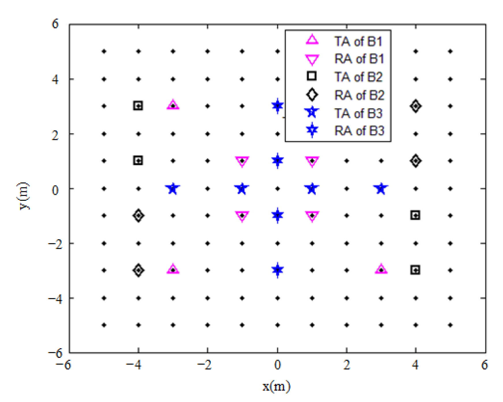
In this section, some target tracking results in relation to varying DOA and Doppler frequency are given to illustrate the effectiveness of the proposed algorithm. The simulation is run on a single Inter (R) Core (TM) i7-4790CPU (3.6 GHz) processor with 4 GB memory, Windows 7 OS. The simulation parameters are shown in Table 2. Assume a colocated MIMO radar with uniformly distributed antennas with 1 m space in a 5 m × 5 m region. The benchmarks for comparison are three fixed antenna configurations: benchmark 1 (B1, annular configuration); benchmark 2 (B2, symmetric configuration); and benchmark 3 (B3, cross-shaped configuration), as shown in Figure 2, where TA means an active transmit antenna, and RA means an active receive antenna. Additionally, each black point in Figure 2 represents an MIMO radar array, which can both transmit and receive signals. The solution yielded by the optimization model (Equation (30)) is also presented for comparison (optimal), which is carried out by the exhaustive search method. The criteria for performance are the square root of the trace of PCRLB, represented by the objective function in Equation (30).
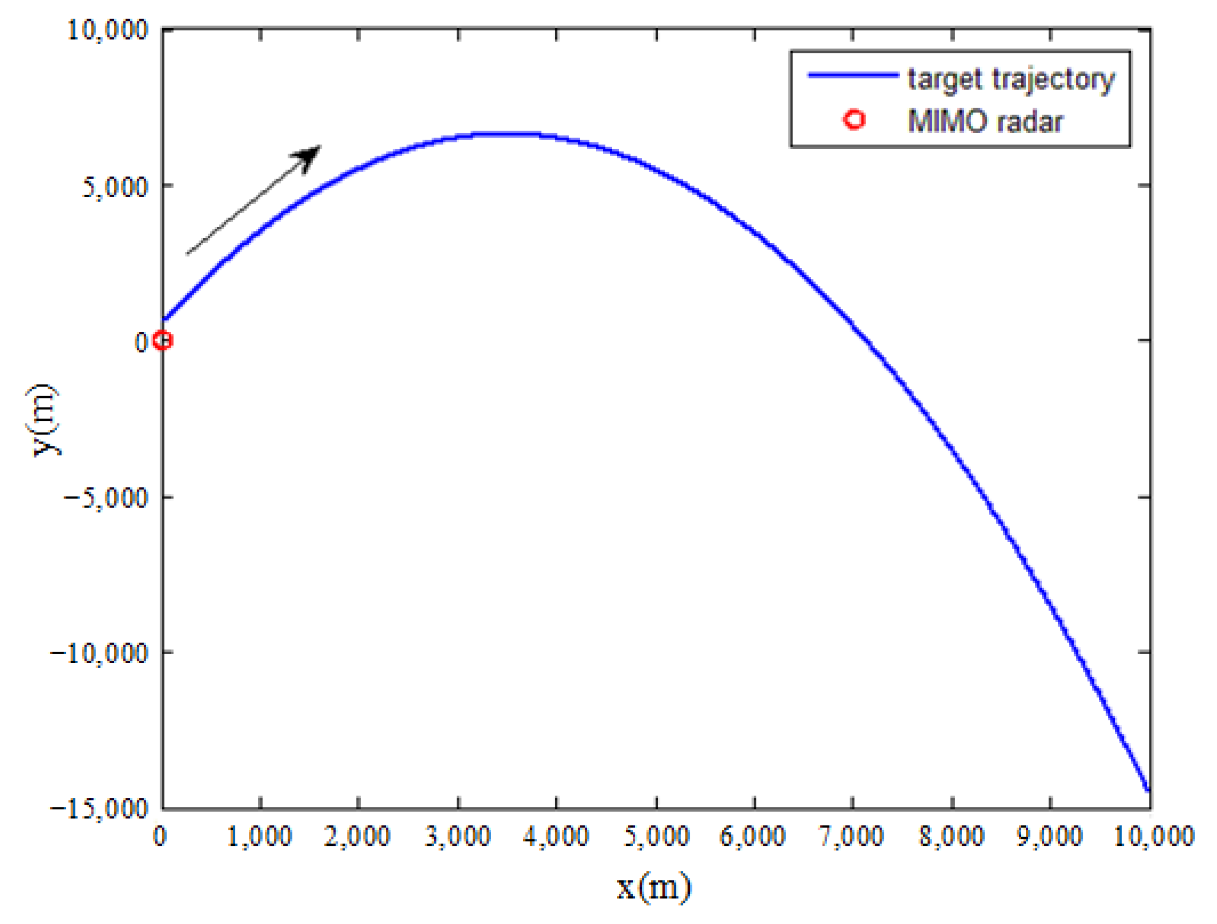
The geometric relationship between the target and the colocated MIMO radar is shown in Figure 3. The target trajectory contains a variety of DOA in the region of [0, π]. The initial state is x = [0, 100, 0, 500, 350, −10]T, and the target moves in the CA model.

5.1. Determining Variable α

In this case, α is regarded as a determining variable. The comparison of performance, obtained by 100 Monte Carlo simulations, is shown in Figure 4 and Figure 5 as well as in Table 3, Table 4 and Table 5.
(1)
Case of SNR = −20 dB
Figure 4. Comparison of the square root of trace of PCRLB.
Remotesensing 14 02912 g004
Figure 5. Computational complexity comparison.
Remotesensing 14 02912 g005
Table 3. Antenna selection of the proposed method in one trial.
Time Epochbt1bt2bt3bt4br1br2br3br4
3(−3,−2)(0,−3)(5,0)(0,1)(2,1)(2,−1)(−4,4)(−2,0)
4(−3,2)(−3,4)(5,2)(1,−4)(4,−3)(1,0)(−4,1)(−1,−2)
5(−4,0)(−4,5)(5,−4)(−3,−3)(2,1)(−1,−1)(0,1)(5,1)
6(2,1)(−5,2)(−1,−5)(5,−1)(4,1)(1,0)(−2,−1)(−4,3)
7(−5,3)(0,4)(4,3)(−4,−3)(4,−1)(3,−2)(−3,0)(1,−4)
Table 4. Comparison of the performance when k|2v2 = 1/100.
AlgorithmsOptimalProposedB1B2B3
Mean square root of trace of PCRLB94.3481105.7771196.2323127.2541312.7999
Table 5. Comparison of runtime (ms).
AlgorithmsProposedOptimalCommon Convex Optimizer
Average runtime 354.929.32 × 10650~200
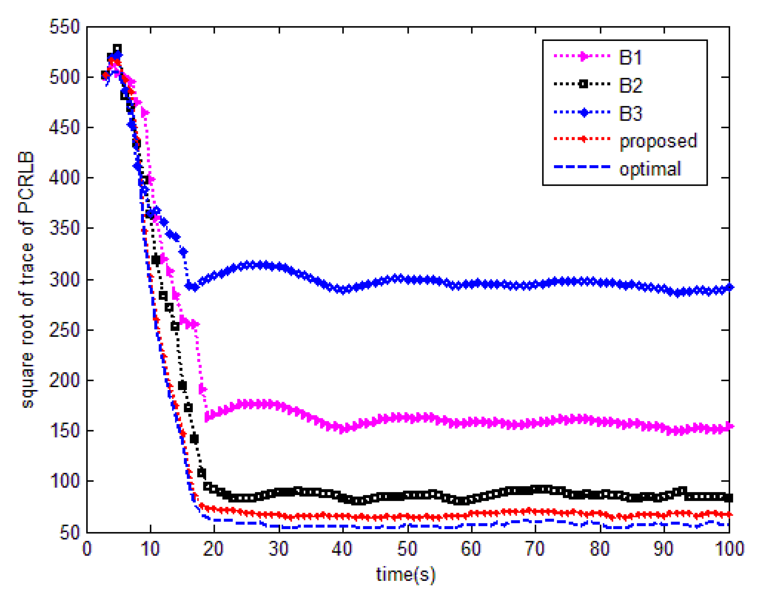
Firstly, the case of k|2v2 = 1/100 (SNR = −20 dB) is studied. Figure 4 shows the square root of the trace of PCRLB of all algorithms. Evidently, on the condition of the same initial estimate error, the dynamic antenna configuration achieves a much lower PCRLB than the three benchmarks. Additionally, it achieves a performance comparable to that of the optimal method. This is because the dynamic antenna configuration can provide the most suitable measurement error, resulting in the minimum PCRLB being achieved in each step. Thereby, the tracking performance is significantly improved. In contrast, the three benchmarks, restricted by the fixed antennas, can only provide constant measurement errors at each step. Such a fixed antenna configuration fails to exploit the target information to the adjust working parameters. As such, a much higher PCRLB is offered.
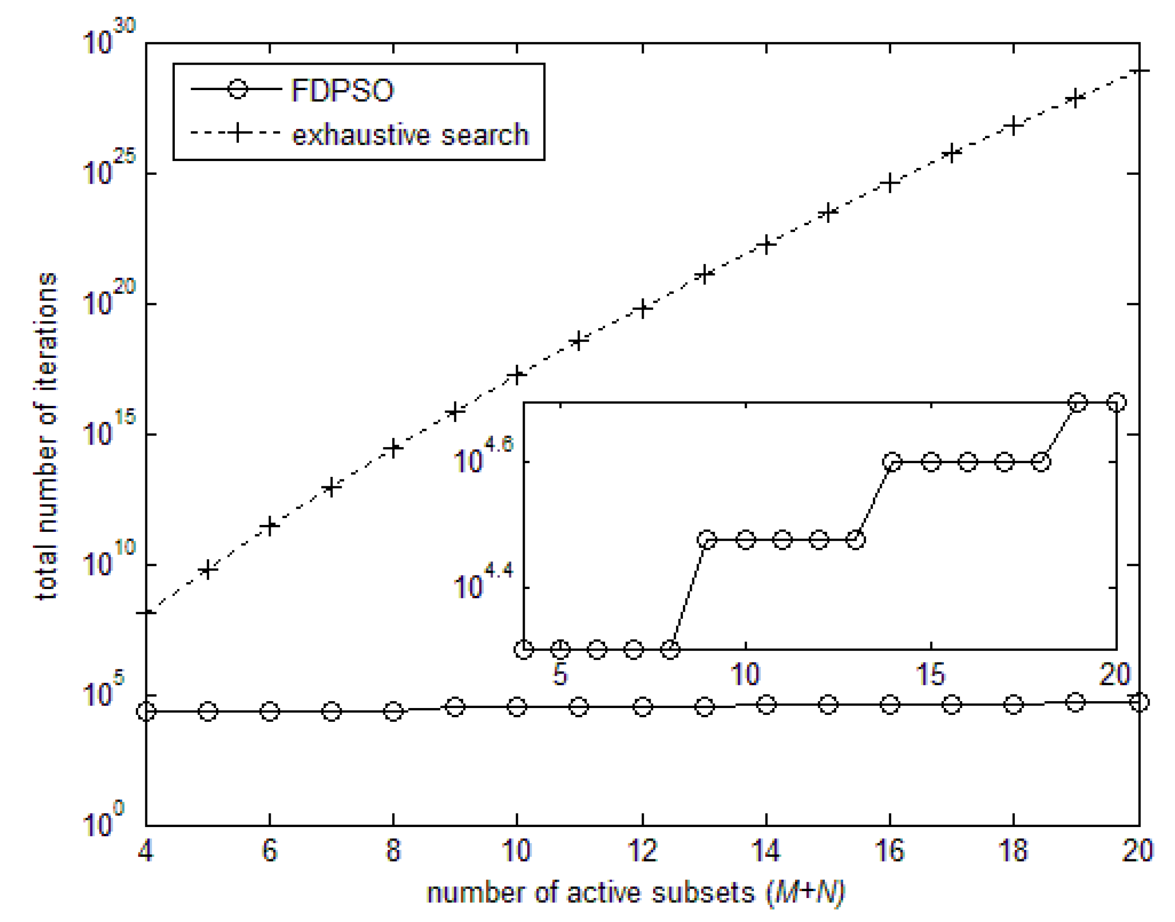
Table 3 presents the antenna placement of the proposed method in one trial. It is obvious that the antennas are dynamically turned to offer a better performance at each time epoch. Moreover, to illustrate the performance improvement, the mean square root of the trace of PCRLB is shown in Table 4. It can be seen that the mean square root of the trace of PCRLB of the proposed method is decreased by 46.10%, 16.88%, and 66.18% on the basis of the three benchmarks, respectively. Though the optimal method achieves a better PCRLB than the proposed method, the performance gap is very narrow. Additionally, the runtime of the two methods shown in Table 5 should be emphasized. For comparison, we also show the runtime of common convex optimizers. It can be seen that the runtime of the optimal method is too long to satisfy the real-time demand. In contrast, the proposed method, which is just a little longer than the common convex optimizer, is fitter for the engineering application. The main reason is that, in the proposed FDPSO, the whole solution region is partitioned into many grid points, leading to a significantly reduced calculation amount. Moreover, a traditional PSO iteration equation is modified by introducing the penalty function and random damping factor. The former item enhances the exploration ability in a rough region, and the latter one forces the particles to search solutions more precisely around the local optima. Therefore, the algorithm can be sufficiently efficient while providing high-quality solutions. To intuitively show the reduction in computational complexity, we plot the total number of iterations of the exhaustive search algorithm and the proposed FDPSO along with the number of active subsets (M + N) in Figure 5.
Evidently, the number of iterations of the exhaustive search algorithm increases exponentially along with the number of active subsets. It brings about a rather large computational burden. In contrast, the complexity of the proposed FDPSO increases only a little, verifying its effectiveness.
(2)
Influence of SNR
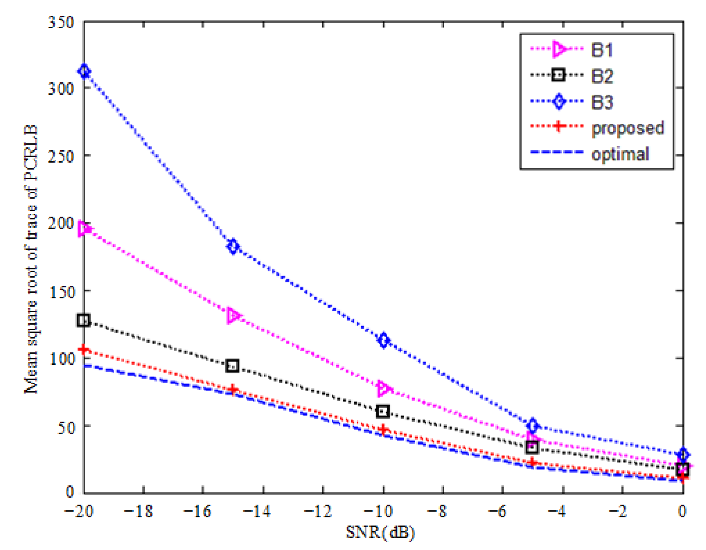
To investigate the influence of SNR on the performance, k|2v2 is tuned from 1/100 to 1 (from SNR = 20 dB to SNR = 0 dB). The simulation result with respect to the mean square root of the trace of PCRLB is shown in Figure 6.
On the condition that SNR is increased, the performance of all the methods is improved. However, the proposed method still performs better than the three benchmarks. Meanwhile, with the increase in SNR, the performance gap between the proposed method and the three benchmarks narrows. This is the same as the conclusion in ref. [7]. However, the differences between ref. [7] and this paper in terms of the scenario and the focused parameters should be highlighted again. In addition, the performance generated by the proposed method is also close to the optimal one, which demonstrates the robustness of the proposed method.

5.2. Random Variable α

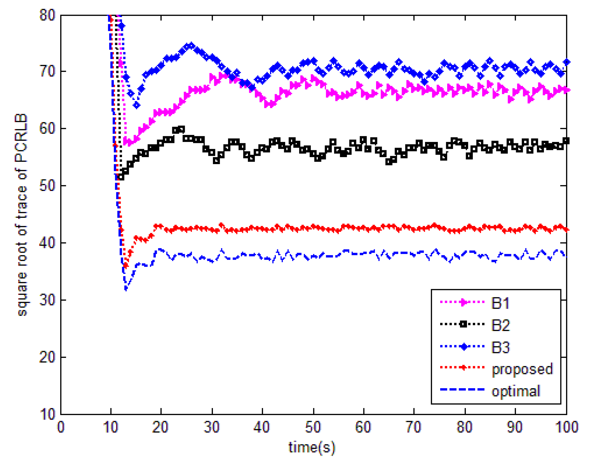
In this case, the target RCS is regarded as a random variable. The performance comparison is shown in Figure 7 and Table 6.
(1)
Case of SNR = −20 dB
Figure 7. Comparison of the trace of PCRLB.
Remotesensing 14 02912 g007
Table 6. Comparison of the performance when k|2v2 = 1/100.
AlgorithmsOptimalProposedB1B2B3
Mean square root of trace of PCRLB53.246357.023685.747777.490389.4255
Figure 7 depicts the PCRLBs obtained by all the methods. In this case, the PCRLBs of the three benchmarks are very close. However, it can be seen again that the proposed method achieves a much lower PCRLB than the three fixed antenna configurations. This is because the proposed method can utilize the closed-loop feedback scheme to adjust the antenna placement, leading to varying measurement errors and the minimum PCRLB being offered at each step. Moreover, the proposed method yields a performance very similar to the optimal one. However, the large calculation demand and long runtime of the latter one, shown in Table 5 and Figure 5, should be again emphasized.
Table 6 compares the mean square root of trace of PCRLB. Compared with the three benchmarks, the proposed method separately improves the PCRLB by 33.50%, 26.41% and 36.23%. In addition, the PCRLB of the proposed method and the optimal one are very close.
(2)
Influence of SNR
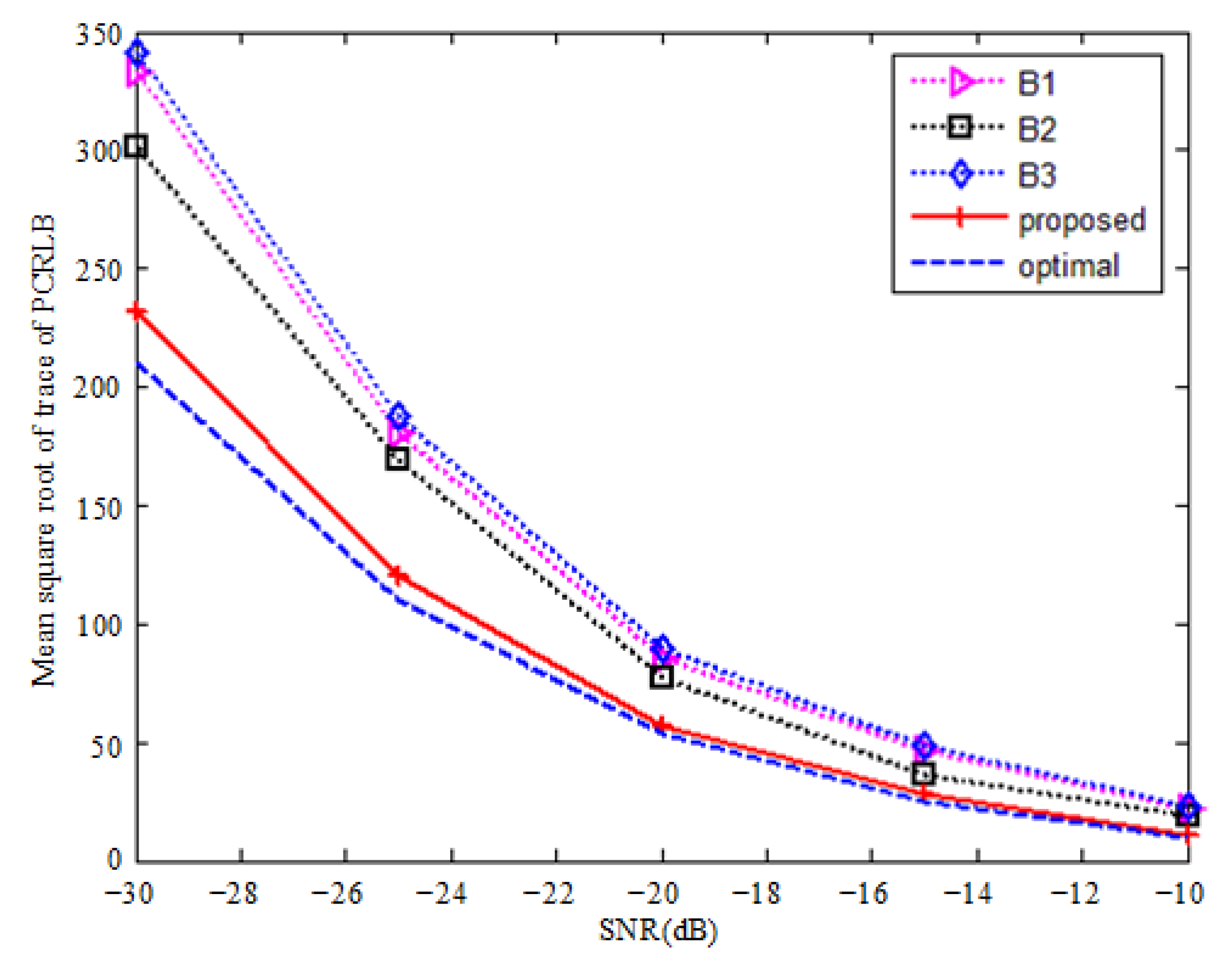
When the SNR = 0 dB, the angle measurement error covariance reaches a very low level (10–14 rad2). Such a low−level measurement error easily leads to filtering divergence. That is because, for tracking targets, the filter needs a little higher error to maintain its performance. Hereafter, we plot the performance comparison where the SNR is from −30 dB to −10 dB in Figure 8.
It is evident that the PCRLBs of all the algorithms are decreased when the SNR is increased. The proposed method always provides a lower PCRLB than the three fixed-antenna configurations, although the performance gap decreases with the increase in SNR. On the other hand, the performance disparity between the proposed method and the optimal one is very small, and it was verified that the proposed method was effective in the low SNR scenario.
Combining the simulation results, some conclusions are drawn as follows:
(1) In the three fixed-antenna configurations, whenever the target RCS is treated as a determining variable or a random variable, B3 always provides the highest PCRLB. Conversely, B2 always achieves the lowest PCRLB.
(2) Under the condition of the same SNR, the performance of all methods when the RCS is as a random variable is better than that achieved by all algorithms when the RCS was the determining variable. This is because the SNR has a higher impact on the PCRLB calculation in the latter case (as can be seen from Appendix A).
(3) Whenever the RCS is regarded as a determining variable or a random variable, the performance gap between the dynamic antenna configuration and the three benchmarks narrows with the increase in SNR.
(4) For target tracking, compared with the three benchmarks, the dynamic antenna configuration can achieve persistent and better performance.
(5) While the exhaustive search method can provide the best performance, the extremely long runtime makes it not applicable for engineering. Conversely, the proposed FDPSO, which is sufficiently efficient and can provide close-to-optimal solutions, is more practical.

6. Conclusions

A novel dynamic antenna adjustment scheme is proposed for the colocated MIMO radar tracking targets. The optimization criterion is the derived PCRLB where the Doppler and DOA information are integrated. Moreover, both the target RCS as the determining variable and the random variable are discussed. The formed optimization problem is not convex, and as such, an efficient FDPSO is proposed for the solution to the problem. Additionally, the cognition technique is introduced, where the obtained target information from the current time epoch is utilized for the PCRLB prediction in next time epoch and guides the antenna placement. Thereby, a closed-loop feedback system is realized where the antenna configuration is self-tuned by perceiving the environment. The simulation results show the following points:
(1) For the three fixed-antenna configurations, the performance differs under the condition that the RCS is regarded as comprised of different kinds of variables and different SNRs.
(2) SNR has a higher impact on performance when the target RCS is treated as the random variable than the determining variable.
(3) The performance gap between the proposed method and three fixed-antenna placements narrows with the increase in SNR.
(4) The proposed dynamic antenna configuration scheme can provide persistent and much better performance than the three fixed-antenna placement.
(5) The proposed FDPSO is sufficiently efficient and can provide close-to-optimal solutions, though a tradeoff between efficiency and optima is implied.
Future work includes the derivation of multi-target PCRLB considering the influence of clutter as well as of more simulations on the Swering II type.

Author Contributions

G.Z. proposed the conceptualization and methodology; Z.L. wrote the draft manuscript; H.Z. and J.X. supervised the experimental analysis and revised the manuscript; C.Q. made contributions to the software. All authors have read and agreed to the published version of the manuscript.

Funding

This research was funded by the National Natural Science Foundation of China, grant number 62001506.

Conflicts of Interest

The authors declare no conflict of interest.

Appendix A. Derivation of R-1 in Swerling I Type

On the condition of Swerling I and Swerling II type, the target’s reflectivity α follows:
α = Σ e j Ω
where Ω follows the even distribution and the PDF of Σ is
p ( Σ ) = 1 σ ¯ e Σ / σ ¯ , Σ 0
In Swerling I type, α remains constant during a pulse train. In contrast, in Swerling II type, α changes from pulse to pulse, and each α is individual.
In Swerling I type, we have
α k , l = α k
p ( α ) = 1 π σ α 2 e α 2 / σ α 2
Combining Equations (7), (13) and (A3), the measurement matrix in time epoch k can be rewritten as
y k = α k G k c I k + v k
where
G k = diag g k , g k , , g k L
c I k = 1 , e j 2 π f d k T p , , e j 2 π f d k ( L 1 ) T p T
where diag{.}L denotes the fact that there are L diagonal elements in the matrix.
(1)
Case 1 for Determining Variable α
From Equation (A5), we have:
p ( y k ξ k ) = 1 π M N L σ v 2 M N L exp y k α k G k c I k 2 σ v 2
and an intermediate variable μIk = αkGkcIk is introduced, then, [p q]th element in Rk1 is:
R DI k 1 p q = 2 σ v 2 Re μ I k H ( ξ k ) p μ I k ( ξ k T ) q
Therefore, when p = 2 and q = 2, we have:
R DI k 1 22 = 2 σ v 2 Re μ I k H θ k μ I k θ k = 2 α k 2 σ v 2 Re c I k H G k H θ k G k θ k c I k
The calculation on ∂GkH/θk is equivalent to ∂gkH/θk, and the latter item is easily obtained as:
g k H θ k g k θ k = 2 π λ 2 m = 1 M n = 1 N cos θ k , sin θ k Δ b m n Δ b m n T × cos θ k , sin θ k T
where
Δ b m n = b t m b r n
Therefore, Equation (A10) is rewritten as:
R DI k 1 22 = 2 α k 2 L σ v 2 2 π λ 2 m = 1 M n = 1 N cos θ k , sin θ k Δ b m n Δ b m n T × cos θ k , sin θ k T
Meanwhile, we have:
R DI k 1 12 = R DI k 1 21 = α k 2 8 π 2 T p L L 1 σ v 2 λ 2   × m = 1 M n = 1 N cos θ k , sin θ k Δ b m n
R DI k 1 11 = 32 α k 2 π 2 T p 2 M N σ v 2 λ 2 L 1 L 2 L 1 6
(2)
Case 2 for Random Variable α
In this case, αk is a complex Gaussian random scalar, and Vk is a complex Gaussian random vector. Therefore, from Equation (A5), Zk also follows complex a Gaussian distribution:
p ( y k ξ k ) = 1 π M N L σ v 2 D I k exp y k H D I k 1 y k σ v 2
where
D I k = σ α 2 σ v 2 G k c I k c I k H G k H + I M N L
Therefore, the [p q]th element in Rk1 is:
R RI k 1 p q = tr D I k 1 D I k ( ξ k ) p D I k 1 D I k ( ξ k ) q
A more clear expression is
D I k 1 = I M N L ( σ α 2 / σ v 2 ) G k c I k c I k H G k H 1 + ( σ α 2 / σ v 2 ) G k c I k 2
D I k ( ξ k ) p = σ α 2 σ v 2 ( G k c I k c I k H G k H ) ( ξ k ) p
when p = 2, Equation (A20) is:
D I k θ k = σ α 2 σ v 2 diag g k θ k g k H , , g k θ k g k H L c I k c I k H + diag g k g k H θ k , , g k g k H θ k L c I k c I k H
and we introduce new notations as:
diag g k θ k g k H , , g k θ k g k H L = A
diag g k g k H θ k , , g k g k H θ k L = B  
diag g k g k H , , g k g k H L = C  
Therefore, when p = 1 and q = 1, Equation (A18) can be rewritten as follows:
R RI k 1 22 = tr D I k 1 D I k θ k D I k 1 D I k θ k = tr I M N L ( σ α 2 / σ v 2 ) C c I k c I k H 1 + ( σ α 2 / σ v 2 ) M N L A c I k c I k H + B c I k c I k H I M N L ( σ α 2 / σ v 2 ) C c I k c I k H 1 + ( σ α 2 / σ v 2 ) M N L A c I k c I k H + B c I k c I k H
R RI k 1 22 = σ α 2 σ v 2 2 tr L A 2 + A B + B A + B 2 c I k c I k H + tr L ( σ v 2 / σ α 2 ) + M N L A C A A C B + B C A B C B c I k c I k H + tr L ( σ v 2 / σ α 2 ) + M N L C A A + C A B C B A C B B c I k c I k H + tr L 2 ( σ v 2 / σ α 2 ) + M N L 2 C A C A C A C B C B C A + C B C B c I k c I k H
It is obvious that the diagonal elements in matrix cIkcIkH are 1; therefore, the analytic expression of Equation (A26) is only related to matrices A, B and C.
Here, we just give the final expression:
R RI k 1 22 = σ α 2 σ v 2 2 2 L 2 M N + 2 L 3 M 2 N 2 ( σ v 2 / σ α 2 ) + M N L 2 π λ 2 × m = 1 M n = 1 N cos θ k , sin θ k Δ b m n Δ b m n T cos θ k , sin θ k T 2 L 2 + 2 L 3 M N ( σ v 2 / σ α 2 ) + M N L + 4 L 4 M 2 N 2 ( σ v 2 / σ α 2 ) + M N L 2 × 2 π λ 2 m = 1 M n = 1 N [ cos θ k , sin θ k ] Δ b m n 2
Similarly, we have
D I k r ˙ k = σ α 2 σ v 2 G k G k H c I k r ˙ k c I k H + G k G k H c I k c I k H r ˙ k
when p = 1 in Equation (A20). After introducing new notations:
c I k r ˙ k c I k H = E , c I k c I k H r ˙ k = F , c I k c I k H = D
we can obtain:
R RI k 1 12 = R RI k 1 21 = tr D I k 1 D I k θ k D I k 1 D I k r ˙ k = σ α 2 σ v 2 2 tr A D + B D C E + C F tr A D + B D C D C E + C D C F ( σ v 2 / σ α 2 ) + M N L tr C D A D + C D B D C E + C F ( σ v 2 / σ α 2 ) + M N L + tr C D A D + C D B D C D C E + C D C F ( σ v 2 / σ α 2 ) + M N L 2
R RI k 1 11 = σ α 2 σ v 2 2 tr D I k 1 D I k r ˙ k D I k 1 D I k r ˙ k = tr M N A E + F 2 tr M 2 N 2 ( σ v 2 / σ α 2 ) + M N L A E + F D E + D F tr M 2 N 2 ( σ v 2 / σ α 2 ) + M N L A D E + D F E + F + tr M 3 N 3 ( σ v 2 / σ α 2 ) + M N L 2 A D E + D F 2
Since the diagonal elements in A are 1, and the analytic expression of Equation (A31) is associated with the diagonal elements in matrices D, E and F. However, it can be demonstrated that they are only connected to parameters Tp, M, N and L, but irrelevant to the antenna configuration. Here, the final expression is given by:
R RI k 1 12 = R RI k 1 21 = 0
R RI k 1 11 = σ α 2 σ v 2 2 16 π 2 T p 2 λ 2 M 2 N 2 L 2 L 2 1 6 M 3 N 3 ( σ v 2 / σ α 2 ) + M N L L 3 L 2 1 6

References

  1. Fishler, E.; Haimovich, A.; Blum, R.S.; Cimini, L.J.; Chizhik, D.; Valenzuela, R.A. Spatial diversity in radars: Models and detection performance. IEEE Trans. Signal Process. 2006, 54, 823–838. [Google Scholar] [CrossRef]
  2. Jian, L.; Stoica, P. MIMO radar with colocated antennas. IEEE Signal Process. Mag. 2007, 24, 106–114. [Google Scholar]
  3. Xu, L.; Li, J.; Stoica, P. Target detection and parameter estimation for MIMO radar systems. IEEE Trans. Aerosp. Electron. Syst. 2008, 44, 927–939. [Google Scholar]
  4. Yu, Y.; Sun, S.; Madan, R.N.; Petropulu, A. Power Allocation and Waveform Design for the Compressive Sensing Based MIMO Radar. IEEE Trans. Aerosp. Electron. Syst. 2014, 50, 898–909. [Google Scholar] [CrossRef]
  5. Bekkerman, I.; Tabrikian, J. Target detection and localization using MIMO radars and sonars. IEEE Trans. Signal Process. 2006, 54, 3873–3883. [Google Scholar] [CrossRef]
  6. Li, J.; Xu, L.; Stoica, P.; Forsythe, K.W.; Bliss, D.W. Range compression and waveform optimization for MIMO radar: A Cramer-Rao bound based study. IEEE Trans. Signal Process. 2008, 56, 218–232. [Google Scholar]
  7. Gorji, A.A.; Tharmarasa, R.; Kirubarajan, K. Optimal Antenna Allocation in MIMO Radars with Collocated Antennas. IEEE Trans. Aerosp. Electron. Syst. 2012, 50, 542–558. [Google Scholar] [CrossRef] [Green Version]
  8. Gorji, A.A.; Tharmarasa, R.; Blair, W.D.; Kirubarajan, T. Multiple unresolved target localization and tracking using collocated MIMO radars. IEEE Trans. Aerosp. Electron. Syst. 2012, 48, 2498–2517. [Google Scholar] [CrossRef]
  9. Yan, J.; Jiu, B.; Liu, H.; Chen, B.; Bao, Z. Prior knowledge based simultaneous multibeam power allocation algorithm for cognitive multiple targets tracking in clutter. IEEE Trans. Signal Process. 2015, 63, 512–527. [Google Scholar] [CrossRef]
  10. Yan, J.; Liu, H.; Jiu, B.; Chen, B.; Liu, Z.; Bao, Z. Simultaneous multibeam resource allocation scheme for multiple target tracking. IEEE Trans. Signal Process. 2015, 63, 3110–3122. [Google Scholar] [CrossRef]
  11. Ming, J.; Liao, G.; Li, J. Joint DOD and DOA estimation for bistatic MIMO radar. Signal Process. 2009, 89, 244–251. [Google Scholar]
  12. Tichavsky, P.; Muravchik, C.; Nehorai, A. Posterior Cramer-Rao bounds for discrete-time nonlinear filtering. IEEE Trans. Signal Process. 1998, 46, 1386–1396. [Google Scholar] [CrossRef] [Green Version]
  13. Xie, M.; Yi, W.; Kong, L.; Kirubarajan, T. Receive-beam resource allocation for multiple target tracking with distributed MIMO radars. IEEE Trans. Aerosp. Electron. Syst. 2018, 54, 2421–2436. [Google Scholar] [CrossRef]
  14. Bishop, A.N.; Fidan, B.; Anderson, B.D.; Doğançay, K.; Pathirana, P.N. Optimality analysis of sensor-target localization geometries. Automatica 2010, 46, 479–492. [Google Scholar] [CrossRef]
  15. Tharmarasa, R.; Kirubarajan, T.; Hernandez, M.L. Large-scale optimal sensor array management for multitarget tracking. IEEE Trans. Syst. Man Cybern. 2007, 37, 803–814. [Google Scholar] [CrossRef]
  16. Tharmarasa, R.; Kirubarajan, T.; Hernandez, M.L.; Sinha, A. PCRLB-based multisensor array management for multitarget tracking. IEEE Trans. Aerosp. Electron. Syst. 2007, 43, 539–555. [Google Scholar] [CrossRef]
  17. Godrich, H.; Petropulu, A.P.; Poor, H.V. A combinatorial optimization framework for subset selection in distributed multiple-radar architectures. In Proceedings of the IEEE International Conference on Acoustics, Speech, and Signal Processing, Prague, Czech Republic, 22–27 May 2011. [Google Scholar]
  18. Godrich, H.; Petropulu, A.P.; Poor, H.V. Sensor selection in distributed multiple-radar architectures for localization: A knapsack problem formulation. IEEE Trans. Signal Process. 2012, 60, 247–260. [Google Scholar] [CrossRef]
  19. He, Q.; Blum, R.S.; Godrich, H.; Haimovich, A.M. Target velocity estimation and antenna placement for MIMO radar with widely separated antennas. IEEE J. Sel. Top. Signal Process. 2010, 4, 79–100. [Google Scholar] [CrossRef]
  20. Song, X.; Zheng, N.; Bai, T. Resource Allocation Schemes for Multiple Targets Tracking in Distributed MIMO Radar Systems. Int. J. Antenn. Propag. 2017, 2017, 7241281. [Google Scholar] [CrossRef] [Green Version]
  21. Haykin, S.; Zia, A.; Xue, Y.; Arasaratnam, I. Control theoretic approach to tracking radar: First step towards cognition. Digit. Signal Process. 2011, 21, 576–585. [Google Scholar] [CrossRef]
  22. Huleihel, W.; Tabrikian, J.; Shavit, R. Optimal Adaptive waveform design for cognitive MIMO radar. IEEE Trans. Signal Process. 2013, 61, 5075–5089. [Google Scholar] [CrossRef]
  23. Chavali, P.; Nehorai, A. Scheduling and power allocation in a cognitive radar network for multiple-target tracking. IEEE Trans. Signal Process. 2012, 60, 715–729. [Google Scholar] [CrossRef]
  24. Garcia, N.; Haimovich, A.M.; Coulon, M.; Lops, M. Resource allocation in MIMO radar with multiple targets for non-coherent localization. IEEE Trans. Signal Process. 2014, 62, 2656–2666. [Google Scholar] [CrossRef] [Green Version]
  25. Martello, S.; Toth, P. Knapsack Problems: Algorithms and Computer Implementations; Wiley: New York, NY, USA, 1990. [Google Scholar]
  26. Eberhart, R.; Kennedy, J. A new optimizer using particle swarm theory. In Proceedings of the Sixth International Symposium on Micro Machine and Human Science, Nagoya, Japan, 4 November 1995. [Google Scholar]
  27. Kennedy, J.; Eberhart, R. Particle swarm optimization. In Proceedings of the IEEE Icnn95-international Conference on Neural Networks, Perth, Australia, 27 November–1 December 1995. [Google Scholar]
  28. Rong, L.; Zhang, L.; Du, B. A novel endmember extraction method for hyperspectral Imagery based on quantum-behaved particle swarm optimization. IEEE J. Sel. Top. Appl. Earth Observ. Remote Sens. 2017, 10, 1610–1631. [Google Scholar]
  29. Liu, L.; Qi, M.S.; Zhou, F. A Novel Non-Uniform Rotational Motion Estimation and Compensation Method for Maneuvering Targets ISAR Imaging Utilizing Particle Swarm Optimization. IEEE Sens. J. 2018, 18, 299–309. [Google Scholar] [CrossRef]
  30. Behnamian, J. Heterogeneous networked cooperative scheduling with anarchic particle swarm optimization. IEEE Trans. Eng. Manag. 2017, 64, 166–178. [Google Scholar] [CrossRef]
  31. Yu, Z.; Xiao, L.; Li, H.; Zhu, X.; Huai, R. Model Parameter Identification for Lithium Batteries Using the Coevolutionary Particle Swarm Optimization Method. IEEE Trans. Ind. Electron. 2017, 64, 5690–5700. [Google Scholar] [CrossRef]
  32. Meza, J.; Espitia, H.; Montenegro, C.; Giménez, E.; González-Crespo, R. González-Crespo, MOVPSO: Vortex multi-objective particle swarm optimization. Appl. Soft. Comput. 2017, 52, 1042–1057. [Google Scholar] [CrossRef]
  33. Valdez, F.; Vazquez, J.C.; Melin, P.; Castillo, O. Comparative study of the use of fuzzy logic in improving particle swarm optimization variants for mathematical functions using co-evolution. Appl. Soft. Comput. 2017, 52, 1070–1083. [Google Scholar] [CrossRef]
  34. Tsai, H.C. Unified particle swarm delivers high efficiency to particle swarm optimization. Appl. Soft. Comput. 2017, 55, 371–383. [Google Scholar] [CrossRef]
  35. Ouyang, H.B.; Gao, L.Q.; Li, S.; Kong, X.Y. Improved global-best-guided particle swarm optimization with learning operation for global optimization problems. Appl. Soft. Comput. 2017, 52, 987–1008. [Google Scholar] [CrossRef]
  36. Lynn, N.; Suganthan, P.N. Ensemble particle swarm optimizer. Appl. Soft. Comput. 2017, 55, 533–548. [Google Scholar] [CrossRef]
  37. Gou, J.; Lei, Y.X.; Guo, W.P.; Wang, C.; Cai, Y.Q.; Luo, W. A novel improved particle swarm optimization algorithm based on individual difference evolution. Appl. Soft. Comput. 2017, 57, 468–481. [Google Scholar] [CrossRef]
  38. Kao, Y.T.; Zahara, E. A hybrid GA and particle swarm optimization for multimodal functions. Appl. Soft. Comput. 2008, 8, 849–857. [Google Scholar] [CrossRef]
  39. Cheng, S.; Zhan, H.; Shu, Z. An innovative hybrid multi-objective particle swarm optimization with or without constraints handling. Appl. Soft. Comput. 2016, 47, 370–388. [Google Scholar] [CrossRef]
  40. Tan, C.; Chang, S.Q.; Liu, L. Hierarchical genetic-particle swarm optimization for bistable permanent magnet actuators. Appl. Soft. Comput. 2017, 61, 1–7. [Google Scholar] [CrossRef]
  41. Arasaratnam, I.; Haykin, S.; Hurd, T.R. Cubature Kalman filtering for continuous-discrete systems: Theory and simulations. IEEE Trans. Signal Process. 2010, 58, 4977–4993. [Google Scholar] [CrossRef]
  42. Glass, J.D.; Smith, L.D. MIMO radar resource allocation using posterior Cramer-Rao lower bounds. In Proceedings of the IEEE Aerospace Conference, Big Sky, MT, USA, 3 May 2011. [Google Scholar]
  43. Zhang, H.; Xie, J.; Ge, J.; Lu, W.; Zong, B. Adaptive Strong Tracking Square-Root Cubature Kalman Filter for Maneuvering Aircraft Tracking. IEEE Access 2018, 6, 10052–10061. [Google Scholar] [CrossRef]
  44. Cui, B.; Chen, X.; Tang, X. Improved cubature Kalman filter for GNSS/INS based on transformation of posterior sigma-points error. IEEE Trans. Signal Process. 2017, 65, 2975–2987. [Google Scholar] [CrossRef]
  45. Zhang, H.; Liu, W.; Zhang, Z.; Lu, W.; Xie, J. Joint target assignment and power allocation in multiple distributed MIMO radar networks. IEEE Syst. J. 2021, 15, 694–704. [Google Scholar] [CrossRef]
  46. Zhang, H.; Liu, W.; Shi, J.; Fei, T.; Zong, B. Joint detection threshold optimization and illumination time allocation strategy for cognitive tracking in a networked radar system. IEEE Trans. Signal Process. 2022, to be published. [Google Scholar]
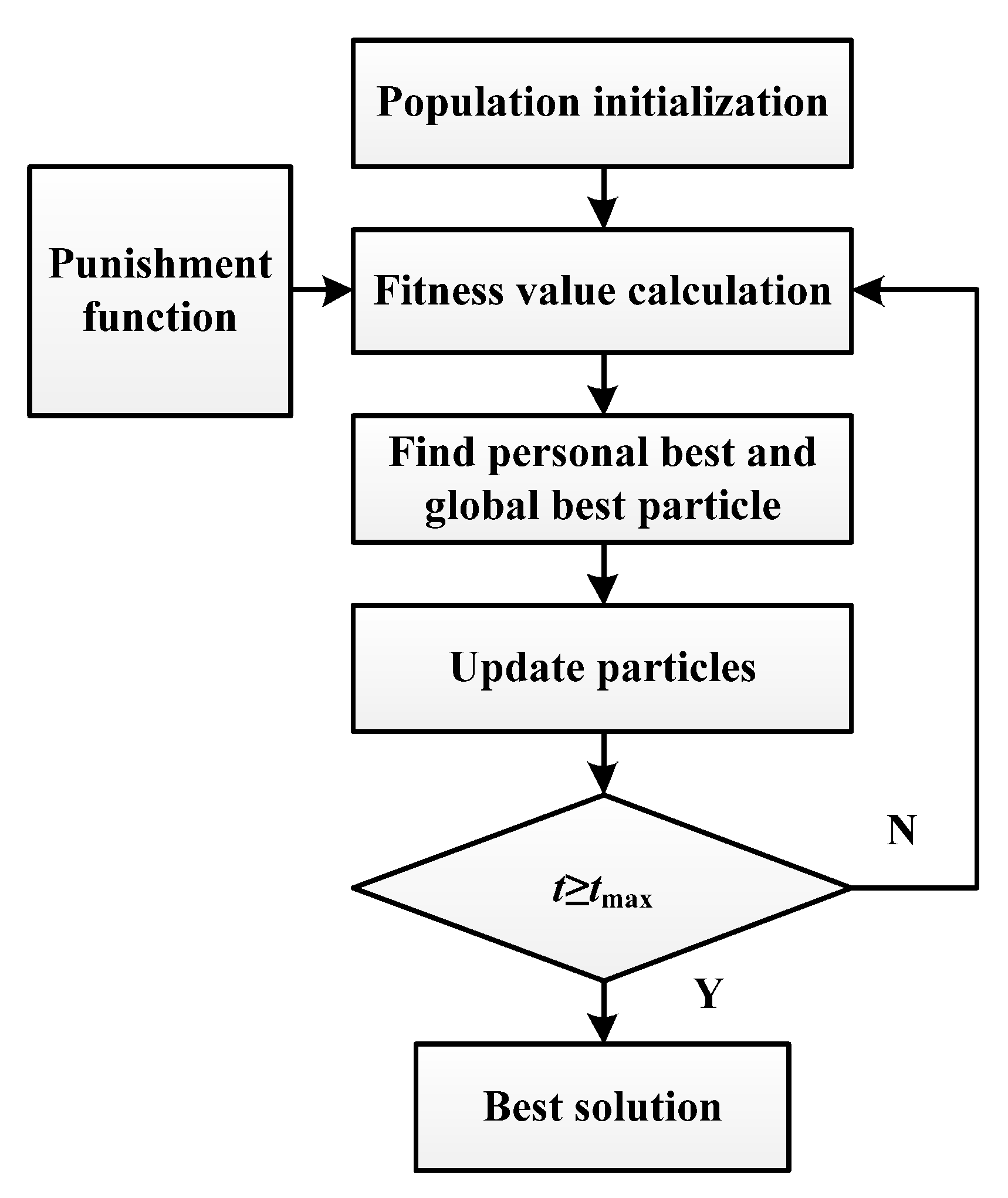
Figure 1. Flow chart of FDPSO.
Remotesensing 14 02912 g001
Figure 2. Antenna configuration of three benchmarks.
Remotesensing 14 02912 g002
Figure 3. Geometric relationship of the targets and MIMO radar.
Remotesensing 14 02912 g003
Figure 6. Mean square root of trace of PCRLB.
Remotesensing 14 02912 g006
Figure 8. Mean square root of trace of PCRLB.
Remotesensing 14 02912 g008
Table 1. Computational complexity comparison.
AlgorithmsExhaustive SearchFDPSO
Computational complexityO (2Mtot+Ntot)O (Npoptmax)
Table 2. Parameters in the scenario.
Ts = 1 sM = 4dmin = 2 mbL = 5 mNpop = 100γ = 0.2Ntot = 121
TP = 0.01 sN = 4dmax = 12 mbU = 5 mtmax = 100ρ = 0.95
nf = 1L = 128λ = 0.2 mΔd = 1 mβ = 0.5Mtot = 121
Publisher’s Note: MDPI stays neutral with regard to jurisdictional claims in published maps and institutional affiliations.