Abstract
Despite the increasing amount of spaceborne synthetic aperture radar (SAR) images and optical images, only a few annotated data can be used directly for scene classification tasks based on convolution neural networks (CNNs). For this situation, self-supervised learning methods can improve scene classification accuracy through learning representations from extensive unlabeled data. However, existing self-supervised scene classification algorithms are hard to deploy on satellites, due to the high computation consumption. To address this challenge, we propose a simple, yet effective, self-supervised representation learning (Lite-SRL) algorithm for the scene classification task. First, we design a lightweight contrastive learning structure for Lite-SRL, we apply a stochastic augmentation strategy to obtain augmented views from unlabeled spaceborne images, and Lite-SRL maximizes the similarity of augmented views to learn valuable representations. Then, we adopt the stop-gradient operation to make Lite-SRL’s training process not rely on large queues or negative samples, which can reduce the computation consumption. Furthermore, in order to deploy Lite-SRL on low-power on-board computing platforms, we propose a distributed hybrid parallelism (DHP) framework and a computation workload balancing (CWB) module for Lite-SRL. Experiments on representative datasets including OpenSARUrban, WHU-SAR6, NWPU-Resisc45, and AID dataset demonstrate that Lite-SRL can improve the scene classification accuracy under limited annotated data, and it is generalizable to both SAR and optical images. Meanwhile, compared with six state-of-the-art self-supervised algorithms, Lite-SRL has clear advantages in overall accuracy, number of parameters, memory consumption, and training latency. Eventually, to evaluate the proposed work’s on-board operational capability, we transplant Lite-SRL to the low-power computing platform NVIDIA Jetson TX2.
1. Introduction
The remote sensing scene classification (RSSC) task aims to classify scene regions into different semantic categories [1,2,3,4,5], which plays an essential role in various Earth observation applications, i.e., land resource exploration, forest inventory, urban-area monitoring [6,7,8]. In recent years, Landsat, Sentinel, and other missions have provided an increasing number of spaceborne images for scene classification task, including synthetic aperture radar (SAR) images and optical images. With more available data, scene classification methods based on convolution neural networks (CNN) have undergone rapid growth [7,9].
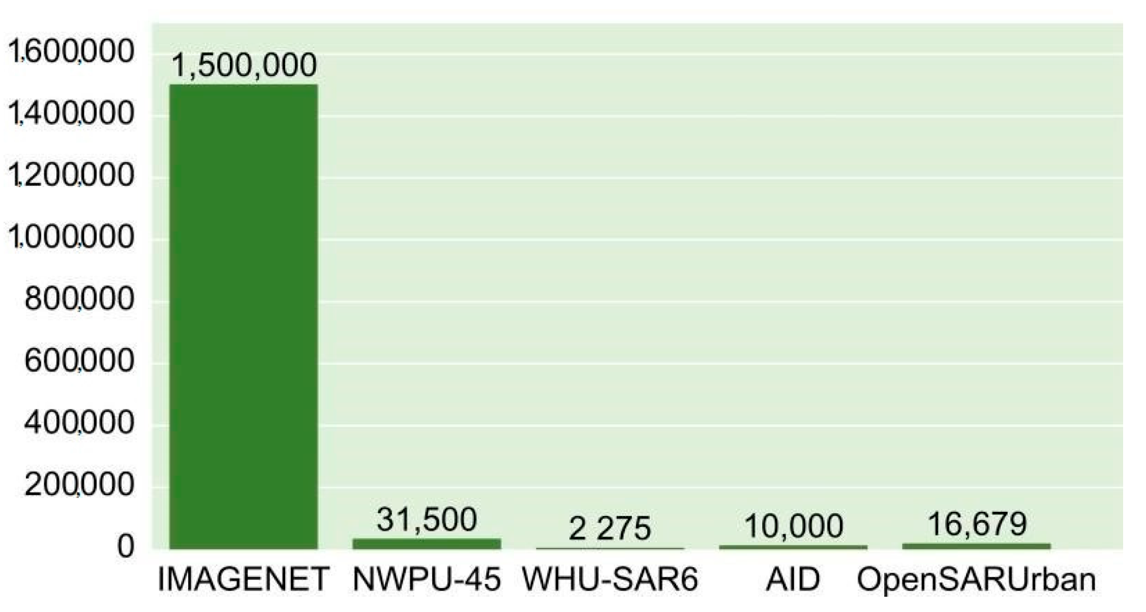
However, the amount of annotated scene data available for supervised CNN training remains limited. Taking SAR data as an example, SAR images are affected by speckle noise due to the imaging mechanism, resulting in poor image quality [10,11]. In addition, the random fluctuation of pixels makes it difficult to distinguish between scene categories [12]. Therefore, the annotation of SAR images requires experienced experts and is a time-consuming task [13]. The same problem of high annotation costs exists for optical images. This leads to the total images number of RSSC datasets, i.e., OpenSARUrban [14], WHU-SAR6 [11], NWPU-Resisc45 [3], and AID [15], compared with natural image datasets, i.e., ImageNet [16], being much smaller; the specific images number for each datasets is shown Figure A1. With limited annotated samples, CNN tends to be overfitted after training [17], leading to poor generalization performance in RSSC task. Therefore, exploring methods to reduce RSSC task’s reliance on annotated data is appealing.
Recently, self-supervised learning (SSL) has emerged as an attractive candidate for solving the problem of labeled data shortage [18]. SSL methods can learn valuable representations from unlabeled images through solving pretext tasks [19]; the network trained in a self-supervised fashion can be used as a pre-trained model to enable higher accuracy with fewer training samples [20]. To this end, an increasing number of RSSC studies have concentrated on SSL. In practice, remote sensing images (RSIs) differ significantly from natural images in the acquisition and transmission stage—RSIs suffer from noise impact and high transmission costs [21]. Performing self-supervised training on satellites can solve these issues; however, existing SSL algorithms are hard to deploy on satellites due to the high computation consumption. The method based on self-supervised instance discrimination [22] was first applied in RSSC task; soon after, the SSL algorithm represented by contrastive multiview coding [20] showed good performance in RSSC tasks. These methods relies on a large batch of negative samples, while the training process needs to maintain large queues, which can consume much computation resources. Other self-supervised methods utilize images with the same geographic coordinate regions from different times and introduce loss functions based on geographic coordinate with complex feature extraction modules [23], which also consume a lot of resources during training. Therefore, we need to reduce the computation consumption during self-supervised training.
As mentioned above, we attempt to deploy a self-supervised algorithm on satellites. A lightweight network is necessary, while a practical on-board training approach can also provide support. Since it is impracticable to carry high-power GPUs on satellites, current trend is to use edge devices, i.e., NVIDIA Jetson TX2 [24] as on-board computing devices [25]. Latest radiation characterized on-board computing modules, such as the S-A1760 Venus [26], utilizes TX2 inside the product to help spacecraft achieve high performance AI computing. Accordingly, we also use TX2 as the deployment platform. As under resource-limited scenarios (limited memory, i.e., memory size of 8 G, limited computation resources, i.e., bandwidth of 59.7 GB/S), distributed strategies are typically applied to train the network; thus, for on-board training a flexible distributed training framework is required. However, the approaches adopted by deep learning frameworks, i.e., PyTorch [27], TensorFlow [28], and Caffe [29], for distributed training remain primitive. Existing dedicated distributed training frameworks, such as Mesh-TensorFlow [30] and Nemesyst [31], are likewise incapable for on-board scenarios, because they fail to consider the case of limited on-board computation resources.
Based on the above observation, we need (i) a self-supervised learning algorithm that satisfies guaranteed accuracy and low computation consumption simultaneously; and (ii) an effective distributed strategy for on-board self-supervised training deployment. To address these challenges, we propose a lightweight On-board Self-supervised Representation Learning (Lite-SRL) algorithm for RSSC task. Lite-SRL uses a contrastive learning structure that contains lightweight modules, by maximizing the similarity of RSIs’ augmented views to capture distinguishable feature from unlabeled images. The augmentation strategies we used to obtain contrast views differ slightly between SAR and optical images. Meanwhile, inspired by self-supervised learning algorithm BYOL [32] and SimSiam [33], we use the stop-gradient operation making the training process not rely on large batch size, queues, or negative sample pairs, which greatly reduces the computation workload with guaranteed accuracy. Moreover, the structure of Lite-SRL is adapted to distributed training for deployment. Experiments on representative scene classification datasets including OpenSARUrban, WHU-SAR6, NWPU-Resisc45, and AID dataset demonstrate that Lite-SRL can improve the scene classification accuracy with limited annotated data; it also demonstrates that Lite-SRL is generalizable to both SAR and optical images in RSSC task. Meanwhile, experiments with six state-of-the-art self-supervised algorithms demonstrate that Lite-SRL has clear advantages in overall accuracy, number of parameters, memory consumption, and training latency.
In order to deploy Lite-SRL algorithm to the low-power computing platform Jetson TX2, we propose a distributed hybrid parallelism (DHP) training framework along with a generic training computation workload balancing module (CWB). Since a single TX2 node cannot complete the whole network training, CWB automatically partitions the network according to the workload balancing principle (View Algorithm 2 for details) and assigns each part to DHP to realize distributed hybrid parallelism training. The integration of CWB and DHP enables training neural networks under limited on-board resources. Eventually, we transplant Lite-SRL algorithm to the on-board computing platform through the distributed training modules.
The main contributions of this article are as follows:
- To improve the scene classification accuracy under insufficient annotated data, we proposed a simple yet effective self-supervised representation learning algorithm called Lite-SRL. To reduce computation consumption, we design a lightweight contrastive learning structure in Lite-SRL and adopt the stop-gradient operation;
- To realize on-board deployment of Lite-SRL algorithm, we proposed a training framework called DHP and a generic computation workload balancing module CWB. As far as we know, we represent the first work to combine self-supervised learning with on-board data processing;
- Extensive experiments on four representative datasets demonstrated that Lite-SRL could improve the scene classification accuracy under limited annotated data, and it is generalizable to SAR and optical images. Compared with six state-of-the-art methods, Lite-SRL had clear advantages in overall accuracy, number of parameters, memory consumption, and training latency;
- Eventually, to evaluate the proposed work’s on-board operational capability, we transplant Lite-SRL to the low-power computing platform NVIDIA Jetson TX2.
The remainder of this paper is organized as follows: Section 2 covers research works related to this article. Section 3 presents the detailed research steps. Section 4 presents the experimental setups. In Section 5 detailed experimental results are presented and summarized. Section 6 provides detailed records for the deployment process. Section 7 provides conclusions. Appendix A lists all the abbreviations in this article and their corresponding full names.
2. Related Works
In this section, we provide a brief review of existing related works. We present solutions of related RSSC works under limited labeled samples, among which, the methods based on self-supervised contrastive learning show excellent results, and we further present the development of self-supervised contrastive learning. We also offer the existing related studies on distributed training.
2.1. RSSC under Limited Annotated Samples
Recently, self-supervised learning (SSL) has attracted considerable interest in the study of RSSC for solving the problem of labeled data shortage. SCL_MLNet [34] introduced an end-to-end self-supervised contrastive learning-based metric network for few-shot RSSC task. Li et al. [35] proposed Meta-FSEO model to improve the performance of few-shot RSSC task in varying urban scenes. These few-shot learning tasks validate that SSL enables RSSC models to achieve well generalization performance from only a few annotated data. Meanwhile, studies [20,36] proved that using the same domain images for SSL training in RSSC task can help to overcome classical transfer learning problems, which further demonstrates the effectiveness of using SSL as a pre-training process in RSSC. The authors of [20,36,37] explored the effectiveness of several SSL networks in RSSC task, among which the contrastive learning-based [22,23] SSL algorithm performed best in the RSSC task. Moreover, Jung et al. [38] presented self-supervised contrastive learning solution with smoothed representation for RSSC based on the SimCLR [22] framework. Zhao et al. [39] introduced a self-supervised contrastive learning algorithm to achieve hyperspectral image classification for problems with few labeled samples. It has been proved by the above works that self-supervised contrastive learning provides a great improvement for RSSC task; thus, our work also adopts the self-supervised contrastive learning method for RSSC task.
2.2. Self-Supervised Contrastive Learning
Through solving pretext tasks, self-supervised methods utilize unlabeled data to learn representations that can be transferred to downstream tasks. In self-supervised learning methods, relative position predicting [19,40], image inpainting [41], and instance-wise contrastive learning [22] are three common pretext tasks. As mentioned above, the validity of contrastive learning is superior to image in-painting and relative position predicting in RSSC tasks. Current state-of-the-art contrastive learning methods differ in detail. SimCLR [22] and MoCo [42] benefit from a large queue of negative samples. Based on earlier versions, MoCo-v2 [43] adds the same nonlinear layer as SimCLR to the encoder representation. MoCo-v2 and SimCLR perform well when maintaining a larger batch. SwAV [44] is another type of clustering-based idea that combines clusters into contrastive learning networks. SwAV computes assignments separately from the two augmented views to perform unsupervised clustering. The clustering-based approach likewise requires large queues or memory banks to supply sufficient samples for clustering. BYOL [32] is characterized by not requiring negative sample pairs and, thus, can eliminate the need to maintain a very large batch of negative sample queues. With no reliance on negative samples, BYOL is more robust to the choice of data enhancement methods. SimSiam [33] is similar to BYOL but with no momentum encoder; meanwhile, it directly shares weights between two branches. SimSiam’s experiments demonstrate that without using any of the negative sample pairs, large batch, and momentum encoders, contrastive learning structures can still learn valuable representations. We applied these methods to RSSC tasks and synthetically compared them with our proposed algorithm.
2.3. Distributed Training under Limited Resources
Distributed training assigns the training process to multiple computing devices for collaborative execution [45]. Current mainstream distributed training methods can be divided into data parallelism [46,47], model parallelism [47,48], and hybrid parallelism [49,50]. In data parallelization, each node trains a duplicate of the model using different mini-batches of data. All nodes contain a complete copy of the model and compute the gradients individually [47], after training the parameters of the final model can be updated through the server. In model parallelization, the network layers are divided into multiple partitions and distributed over multiple nodes for parallel training [47,49]. During model parallelization training, each node has different parameters and is responsible for the computation of different partition layers, and each node updates only the weights of assigned partitions. Hybrid parallelism is a combination of data parallelism and model parallelism, which is the development trend of distributed training. Mesh-TensorFlow [30] and Nemesyst [31] are two end-to-end hybrid parallel training frameworks, both using small independent batches of data for training. Based on Mesh-TensorFlow, Moreno-Alvarez et al. [51] proposed a static load balancing approach for the model parallelism scheme. Akintoye et al. [49] proposed a generalized hybrid parallelization approach to optimize partition allocation on available GPUs. FlexFlow [47] framework applied a simulator to predict optimal parallelization strategy in order to improve training efficiency on GPU clusters. However, the above distributed training frameworks failed to consider resource-limited scenarios; in addition, they do not perform computation workload balancing for training process.
3. Methods
3.1. Overview of the Proposed Framework
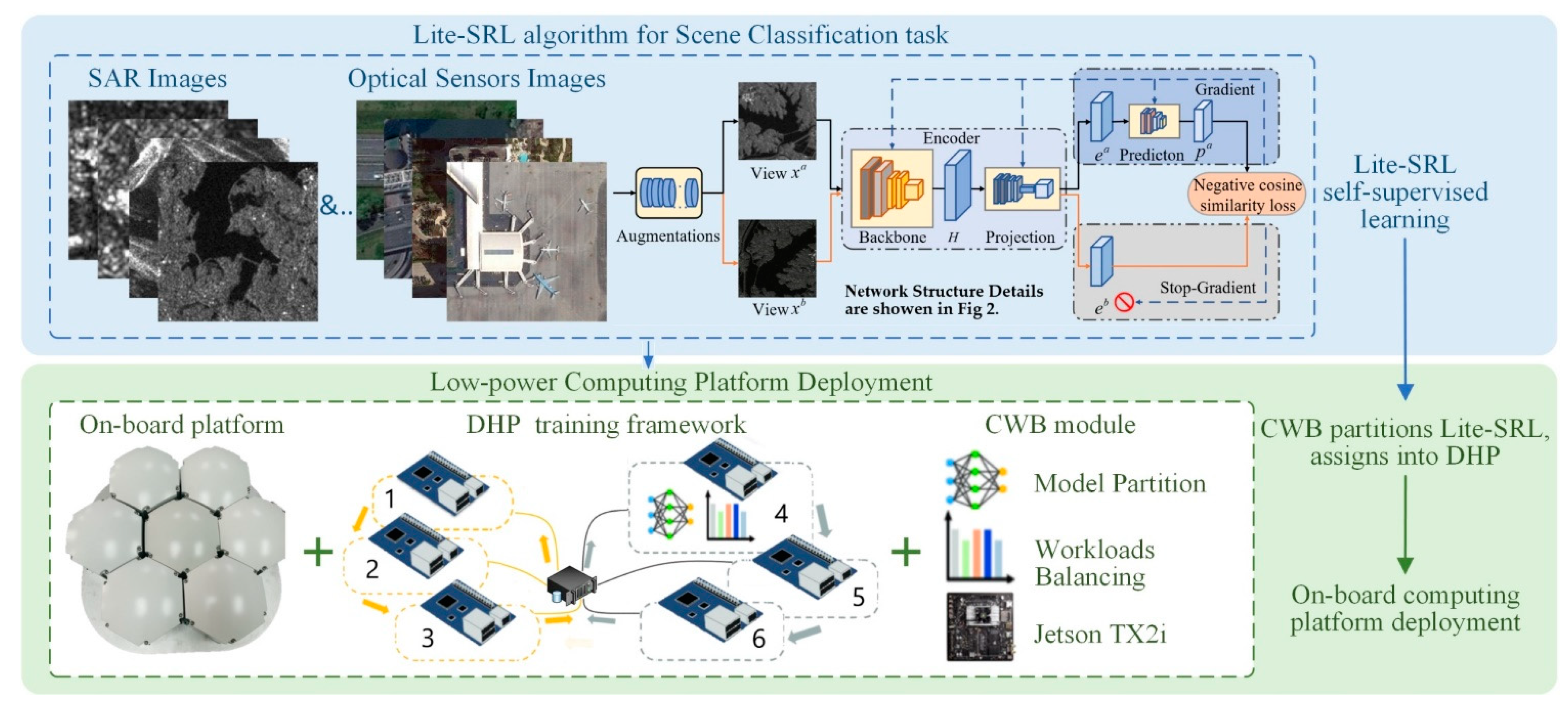
The overview of the proposed work is shown in Figure 1; our work consists of two main parts: (i) we propose a self-supervised algorithm Lite-SRL for RSSC task, the algorithm satisfies guaranteed accuracy and low computation consumption simultaneously. (ii) We use a low-power computing platform for deployment and we propose a set of distributed training modules to satisfy the requirements.
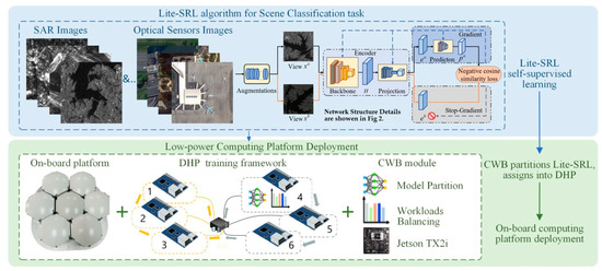
Figure 1.
Overview of the proposed work. Lite-SRL: on-board self-supervised representation learning algorithm for RSSC task; CWB: computation workload balancing module; DHP: on-board distributed hybrid parallelism training framework.
To improve the scene classification accuracy with limited annotated data, Lite-SRL learns valuable representations from unlabeled RS images. During the algorithm deployment, CWB automatically partitions the training process of Lite-SRL according to the workload balancing principle (View Algorithm 2 for details) and assigns each partition into the DHP training framework, achieving high efficiency on-board self-supervised training.
3.2. Lite-SRL Self-Supervised Representation Learning Network
3.2.1. Network Structure
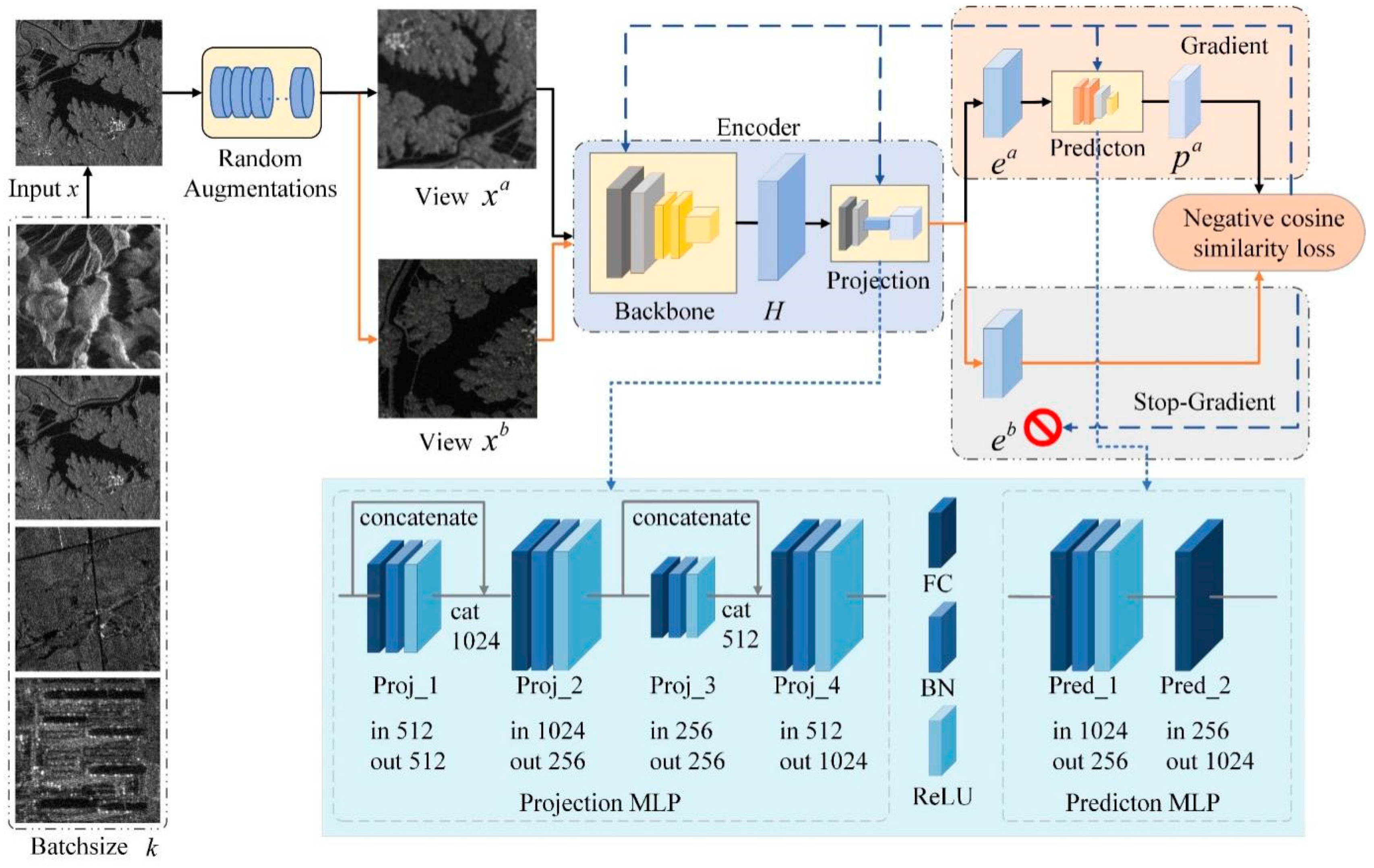
We propose an On-board Self-supervised Representation Learning (Lite-SRL) network for RSSC tasks. Since SimSiam [33] and BYOL [32] have excelled as effective self-supervised contrastive learning methods for many downstream tasks, we use a similar structure as the pretext task for self-supervised contrastive learning and make the training process less resource-intensive. Based on SimSiam’s experiment results, our Lite-SRL directly maximizes the similarity of two augmented views of an image without using either negative pairs or momentum encoders, and, thus, the training process does not rely on large batches or queues. Lite-SRL adopts lightweight structures as detailed in Figure 2, allowing us to achieve high accuracy with fewer parameters and training resource usage.

Figure 2.
Network structure.
The structure of Lite-SRL is shown in Figure 2, where two randomly augmented views and are obtained from the training batch as inputs, with the top and bottom paths sharing the parameters of Encoder. These two views are processed separately by encoder E, which consists of Backbone and Projection. Prediction is denoted as P, it converts the output of one view after encoder and matches it with the other view. Express the output vectors of and are expressed as and . Again, perform the above procedure in reverse order for and , the output vectors are and . Vectors’ negative cosine similarity is expressed as follows:
here is l2-norm, . The symmetrization loss is expressed as follows:
using Equation (1) to simplify the symmetrization loss calculation, Equation (2) yields the following equation:
The overall loss during training is the average of all images in the batch. The study of SimSiam and BYOL demonstrated that the stop gradient operation is the key to avoid collapse during training. More importantly, stop gradient operation allows the training process to not rely on large batch size, queues, or negative sample pairs, which greatly reduces the computation workload. We also use the Stop-Grad operation, as shown in Figure 2, for the way that does not go through P we apply stop gradient operation to it when performing back propagation, modifying (1) as follows:
which means is considered as a constant in this term. By adding Stop-Grad operation, the form in Equation (3) is realized as:
The encoder of in the first term of Equation (5) does not receive the gradient from , instead receives the gradient from in the second term, and the operation performed on the gradient of is opposite to that of . After obtaining the contrastive loss, we use the stochastic gradient descent (SGD) optimizer to perform back propagation and update the network parameters. The learning procedure is formally presented in Algorithm 1. The structure of the Projection and Prediction multi-layer perceptron (MLP) modules in Lite-SRL are shown in Figure 2. We use lightweight MLP modules, each fully connected layer in Projection MLP is connected to batch normalization (BN) layer and rectified linear unit (ReLU), we incorporated two concatenate layers in the structure. Prediction MLP uses a bottleneck structure, as detailed in Figure 2. Neither BN nor ReLU is used in the last output layer, and such a structure prevents training collapse [39,44].
| Algorithm 1. Learning Procedure of Lite-SRL |
| E: Encoder with |
| P: Prediction MLP Aug: random image augmentation |
| : parameters of E and P Stop: stop-gradient operation Input: Training samples Output: negative cosine similarity loss |
| 1: for number of training epochs do |
| 2: Training samples in a minibatch form |
| 3: Do augmentation 4: In Lite-SRL 2-way do and ; and 5: Calculate negative cosine similarity with stop-gradient operation 6: Do backwards propagation with SGD optimizer 7: Update weights 8: end for 9: After training, use pre-trained model for downstream Remote Sensing Scene Classification |
Lite-SRL uses a simple, yet effective, network structure, which has significant advantages over existing self-supervised algorithms in (i) network parameters, (ii) memory consumption, and (iii) the average training latency. Detailed experimental results are shown in Section 5.1.
3.2.2. Lite-SRL Network Partition
In order to deploy the algorithm on low-power computing platforms, the training process of Lite-SRL is adapted to a sequential structure as shown in Figure 3a. For two views, and , of an augmented image, first perform concatenate operation and send them to Encoder together, get the combined output of and , keep the values of and and do not preserve the gradient information. Then send them to Prediction part and get and , use the retained and when calculating the contrastive loss with and , considering or as constant values when applying the stop-gradient operation. This allows the two contrastive losses to be calculated simultaneously.
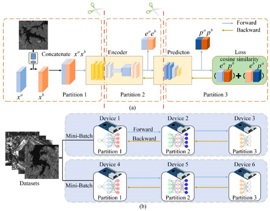
Figure 3.
(a) We design the training process of Lite-SRL as a sequential structure to adapt model parallelization. (b) Schematic of the proposed distributed hybrid parallel (DHP) training baseline.
Each convolution layer within a CNN structure can be used as a single partition to achieve highly efficient model parallelism training capabilities. Given a network M that consists of layers . Divide network M into n partitions where , denotes partition is start from layer and contains k layers. Except for this, the calculation of all partitions is sequential, partition transmit its output feature to its next partition , while the gradient calculated by partition is transmitted to the front partition . At iteration t, during forward propagation send the input from partition to partition and delivers activation . Identically, during backward propagation of iteration t, the indicates the gradient calculated by partition . With each layer , we denote the weight parameter of layer as , the gradient is given as:
We denote the learning rate as , Equation (6) is updated by the following equation:
For layers in non-sequential CNN, parallel paths are not partitioned; instead the parallel zone is considered as a block. After the network partitioning, the network can be trained in model parallelism mode.
In Figure 3b, the feature and gradient are transferred between devices. Take Device 1 and Device 2, for example; Device 1 is in charge of Partition 1’ s training and Device 2 is in charge of Partition 2’ s training. In iteration t, during forward propagation, the last layer of Partition 1 in Device 1 transmits feature value to the first layer of Partition 2 in Device 2. During backward propagation, Device 2 transmits the gradient value to Device 1, the gradient of Partition 1′s last layer is , where is the weight parameter of Partition 1′s last layer obtained from iteration t − 1. Device 1 updates the weight parameters according to Equations (6) and (7): ,where is learning rate.
3.3. Distributed Training Strategy
We use a combination of six TX2 nodes and one high-speed switch to form the low-power computing platform as shown in Figure 15.
With multiple nodes, different amounts of nodes can be flexibly scheduled to participate in the training according to the computing requirements. We propose a distributed hybrid parallelized DHP training framework based on the PyTorch framework, the schematic of DHP is shown in Figure 3b. DHP framework uses TCP communication protocol, and the data transmitted between nodes mainly include the output feature of each layer in the forward propagation, the gradient values obtained from each layer in backward propagation, and the parameters of layers aggregated by each node after reaching the number of iterations. Meanwhile, we propose a generic computation workload balancing module CWB, which can perform model partitioning and workload balancing for a given network structure and working conditions. CWB is the core that enables training CNN under limited computing power. Furthermore, based on our DHP framework, we propose a dynamic chain system that can promote the training speed without sacrificing training accuracy.
3.3.1. Computation Workload Balancing Module
Under model parallelism, each node has different parameters and is responsible for the computation of different model layers respectively, updating only the weights of the assigned model layers. Setting appropriate network partitioning points for network partitioning can improve the efficiency of distributed training. TX2 uses Jetson series SOC, with CPU and GPU sharing 8 GB memory and the memory requirements during Lite-SRL training process are larger than the computing capacity of a single TX2; thus, network partitioning and workload balancing are required.
We propose a gen*eric Computation workload Balancing module, CWB; it works as follows. For a given network structure and specified batch of input data, take Lite-SRL as an example. Lite-SRL contains a total of q layers of networks ; CWB first collects the forward inference and back propagation time of each layer running on TX2, where the forward inference time of each layer is denoted as , and the back propagation is denoted as . CWB then calculates the memory size occupied by the model parameters of each layers , and the memory size occupied by the output of the intermediate layers . CWB partitions Lite-SRL into n partitions and assigns them to n TX2 , where , then between and , that is, between and need to transmit the feature data from layer to layer , and the gradient value needs to be transmitted back during back propagation. Record the ratio of the file size to the transmission rate between TX2 as the theoretical transmission latency , CWB calculates the transmission latency for all candidate partition points.
The training time for a mini-batch is:
The equation for calculating the equipment utilization index is as follows:
The process of CWB searching for the best partition point is formally presented in Algorithm 2. After network partitioning, each partition is assigned to the DHP system for distributed training. The detailed implementation of CWB is recorded in Figure 13.
| Algorithm 2. CWB search for the best partition point |
| Step1:CWB performs memory workload balancing Step2:CWB performs time equalization 1: Assign and to 2: Assume 3 TX2s can satisfy memory allocation, then 2 sets of candidate partition point that satisfy memory workload balancing are recorded as |
| 3: for a in do 4: for b in do 5: Partition point 1 adopts a, partition point 2 adopts b 6: Denote the running time of as 7: Denote the running time of as 8: Denote the running time of as |
| 9: The training time for a mini-batch is |
| 10: The partition point use , the ratio of running time to waiting time of is |
| 11: Calculate the equipment utilization indices E using Equation (9) 12: end for 13: end for 14: The partition point of E with the highest score is the best partition point |
3.3.2. Dynamic Chain System
Figure 4a shows our hybrid parallel distributed training baseline schematic, where each node in the chain is fixedly linked to its front and back nodes, and the later nodes in the chain have to wait for the front nodes to finish forward and backward propagation. Overlap network computation time with transmission time is a common method to improve efficiency in distributed training [52], which can improve training efficiency. Our modified dynamic chain is shown in Figure 4b, where three nodes are responsible for the computation of partition 1, two for the computation of partition 2, and one for the computation of partition 3 of the model. We add a communication scheduler module to our distributed training framework, enabling the node that first completes the computation to search for the available nodes in the next layer. Each mini-batch will form a dynamic chain that performs forward and backward propagation, and after each node completes its current backward propagation, it will automatically leave the current chain and construct a new chain with the node that is waiting. Dynamic chain system has higher training efficiency than baseline, improving node utilization without reducing training accuracy. The dynamic chain system can be well generalized for different training demands, and we have conducted additional experiments for different training computations as detailed in Section 6.2.
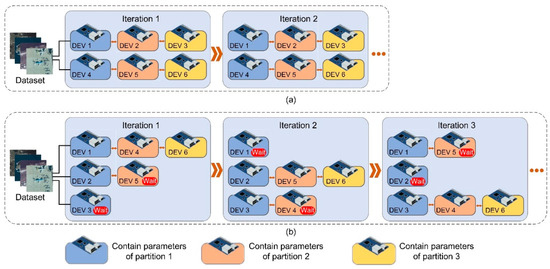
Figure 4.
Illustration of our proposed distributed hybrid parallel training baseline and dynamic chain system. (a) Distributed hybrid parallel training baseline. (b) Dynamic chain system. In iteration 1, Devices 1, 4, and 6 forms a computation chain, while Devices 3 and 5 are in a waiting state. During this time, Device 5 completes the forward computation from Device 2. At the end of iteration 1, Device 6 disconnects from Device 4, automatically links to Device 5, and immediately performs the third part of the training, Device 4 links to Device 3 and waits to link with Device 6. In iteration 3, Device 4 links to Device 6, and the rest nodes also link to available nodes. Subsequent iterations follow the same procedure.
4. Experimental Setups
4.1. Datasets Description
For SAR images, we use the OpenSARUrban [14] dataset and the WHU-SAR6 [11] dataset for experiments. We use a small number of training samples to predict a large number of test samples in our experiments, the training proportions for OpenSARUrban dataset are 10% and 20%, and for WHU-SAR6 dataset we set training proportions as 10% and 20%.
- The OpenSARUrban [14] dataset consists of 10 categories of urban scene images collected from Sentinel-1; its scene images cover 21 major cities in China. Each category contains about 40 to 2000 images with a size of 100 × 100 pixels, and the resolution of the images is about 20 m;
- The WHU-SAR6 [11] dataset consists of six categories of scene images collected form Sentinel-1 and GF-3. Each category contains about 250 to 420 images with ranging in size from 500 to 600 pixels. Since the total number of WHU-SAR6 images is relatively small, to increase the dataset volume we crop the images into small patches of 256 × 256 pixels without destroying the scene semantic information.
For optical images, we use the NWPU-RESISC45 [3] dataset and the Aerial Image dataset (AID) [15]. The training proportions for NWPU-RESISC45 dataset are 10% and 20%, which are more challenging since they both require using a small number of training samples to predict labels for many test data. For the AID dataset, we set training proportions as 10%, 20%, and 50%. Detailed information is shown in Table 1.

Table 1.
Datasets description and training proportions.
- The NWPU-RESISC45 [3] dataset is the current largest open benchmark dataset for scene classification task, consisting of 45 categories of scene images. Each category contains 700 images with a size of 256 × 256 pixels, and the spatial resolution of the images is about 0.2 to 30 m.
- The AID [15] dataset consists of 30 categories of scene images; each category containing about 200 to 400 images, for a total of 10,000 samples, each with a size of 600 × 600 pixels.
4.2. Data Augmentation
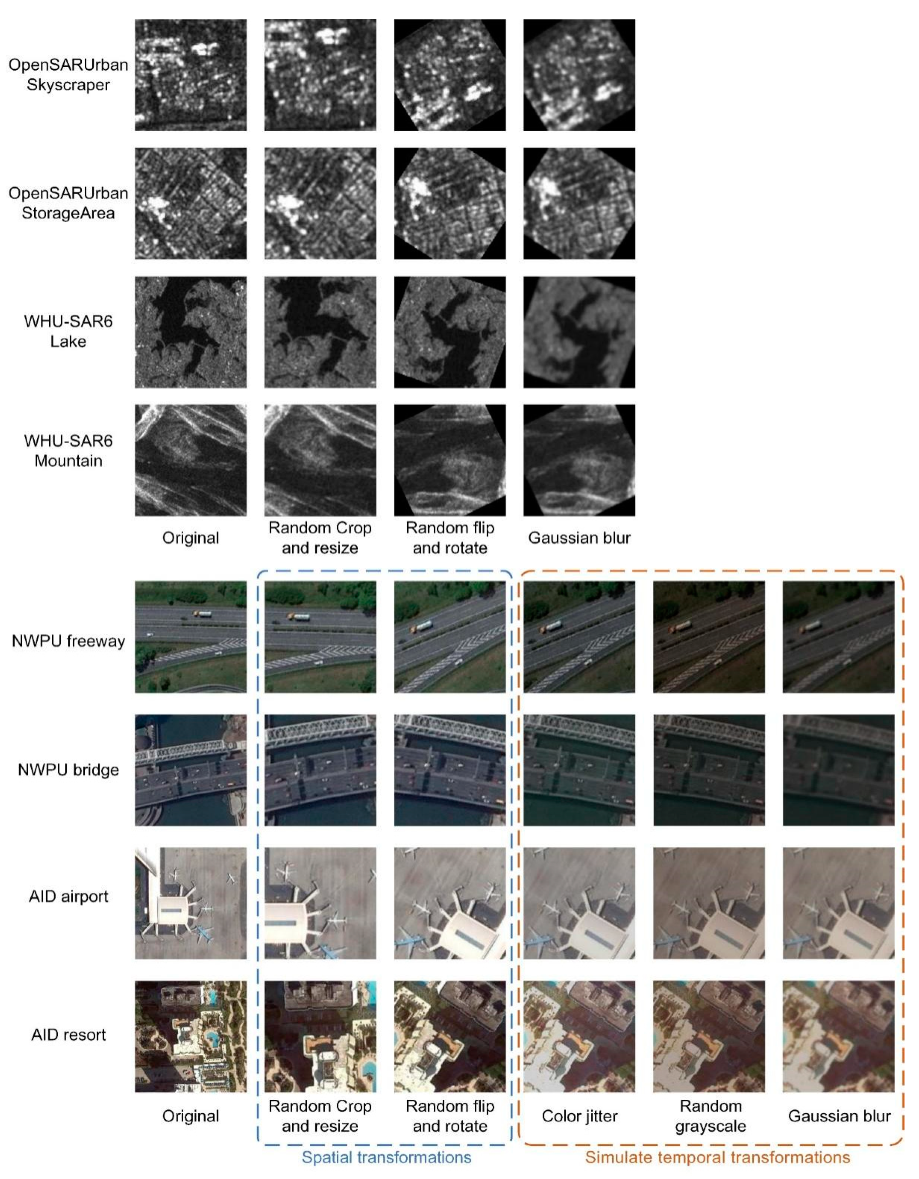
By performing random crop and resize on target image, the receptive field of the network can achieve both global and local prediction, which is crucial for RSSC task. We perform spatial transformations such as random crop, flip, rotate, and resize to enable the model to learn rotation invariants and scaling invariants simultaneously. Further, we simulate temporal transformations with Gaussian blur, color jitter, and random grayscale. The augmentation strategies differ between SAR images and optical images. Detailed data augmentation result is shown in Figure 5.
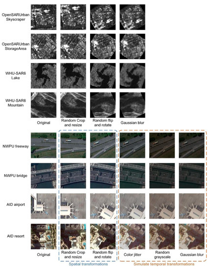
Figure 5.
Illustration of data augmentations.
4.3. Implementation Details
The input images were normalized to 224 × 224 and used the data augmentation settings shown in Figure 5. The batch size was set to 64, and all methods were trained for 400 epochs. For all competitive algorithms, we used ResNet-18 [53] as the backbone and removed the fully connected layer after Advpooling in ResNet-18. Since the loss functions and optimizers of these competitive methods are different, the experimental results are obtained under the individual methods’ respective optimal hyperparameter settings. All competitive algorithms were implemented using PyTorch 1.7, Python3.7. The proposed Lite-SRL method used an SGD optimizer with a momentum of 0.9 and a weight decay of 1 × 10⁻⁴, the initial learning rate was 0.05, and the learning rate decreased using the cosine decay.
The experimental section consists of two parts.
- Experiments of self-supervised learning. In this part we use workstations to compare the proposed Lite-SRL with other advanced self-supervised methods comprehensively. The two workstations are identically configured with NVIDIA RTX 3090GPU, Intel Xeon CPU E5-1650, and 64 G RAM.
- Experiments for on-board deployment of Lite-SRL algorithm. We used the proposed distributed training modules and provided detailed records for the deployment process. The experimental on-board computing platform consists of NVIDIA Jetson TX2 nodes and a high-speed switch.
5. Experimental Results
The flowchart of self-supervised learning experiments is shown in Figure 6. Encoders obtained by self-supervised training are used both as (i) frozen feature extractors (Freeze experiment), and as (ii) initial fine-tune model (Fine-tune experiment). For both the freeze and fine-tune experiments, we connected a linear classifier after the encoder and used an Adam optimizer with a batch size of 64, the learning rate reduced in a cosine manner within 200 epochs.
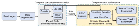
Figure 6.
The flowchart of self-supervised learning experiments.
5.1. Guaranteed Accuracy with Less Computation
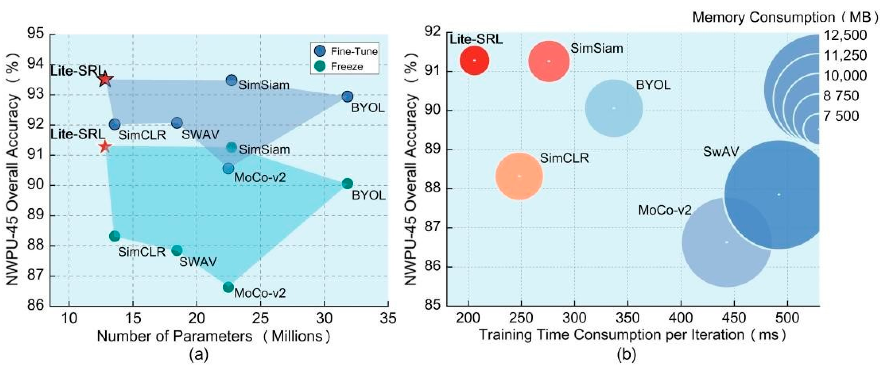
We compare (i) overall accuracy, (ii) number of parameters, (iii) memory consumption, and (iv) average training latency with competitive self-supervised algorithms. The memory consumption during network training consists of the following elements. The memory occupied by the model: including the consumption of parameters, gradients and optimizer momentum. The memory occupied by the network intermediate layers’ outputs: including the inputs and outputs of each layer.
Considering that on-board scenario is highly sensitive to the computation workload, the algorithm is required to achieve higher accuracy and less computation simultaneously. Experiments show that Lite-SRL can achieve optimal classification accuracy with minimum computation. As shown in Figure 7, Lite-SRL shows the best accuracy in the RSSC task, while Lite-SRL has a clear advantage in terms of computation consumption. Thus Lite-SRL provides a lightweight yet effective solution for on-board self-supervised representation learning.
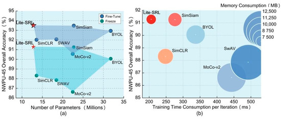
Figure 7.
Guaranteed accuracy with less computation. (a) Fine-tune and freeze experiment results on NWPU-45 dataset with training proportion of 20%, the horizontal axis compares the number of parameters. (b) Freeze experiment results on NWPU-45 dataset with training proportion of 20%; horizontal axis compares the training time consumption per iteration, and the diameter of the bubble is proportional to the memory consumption during network training.
5.2. Self-Supervised Representation Extractor
In freeze training experiment, we use the encoders obtained from each method as feature extractors to evaluate their performance in scene classification. To visualize the effectiveness of Lite-SRL, we fed the test set images to the pre-trained model learned from Lite-SRL, and applied t-SNE [54] to map the output features to a 2-dimensional space. As shown in Figure 8, features from different classes can be well distributed by our self-supervised method, with significantly better results than ImageNet supervised pre-trained model. This demonstrates that by utilizing unlabeled RSI data, our proposed representation learning strategy enables the model to produce a valuable feature representation for downstream RSSC task.
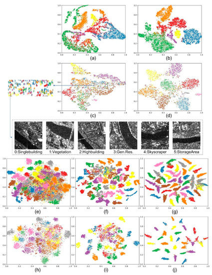
Figure 8.
The t-SNE visualization of feature distributions on different datasets. (a) Lite-SRL model on WHU-SAR6 dataset; (b) fine-tuned Lite-SRL model on WHU-SAR6 dataset; (c) Lite-SRL model on OpenSARUrban dataset; (d) fine-tuned Lite-SRL model on OpenSARUrban dataset; for SAR dataset due to the imaging mechanism, we did not use ImageNet’s pre-trained model. (e) ImageNet pre-trained model on NWPU-45 dataset; (f) Lite-SRL model on NWPU-45 dataset; (g) fine-tuned Lite-SRL model on NWPU-45 dataset; (h) ImageNet pre-trained model on AID dataset; (i) Lite-SRL model on AID dataset; (j) fine-tuned Lite-SRL model on NWPU-45 dataset.
In Figure 8c, we marked the samples from the OpenSARUrabn dataset that Lite-SRL failed to distinguish. We found that these SAR samples contain confusable features. For instance, the six different scene categories in Figure 8c all contain a river flowing through the city. Since we do not use any labels during self-supervised learning, Lite-SRL may extract the wrong features for these confusing scene images.
Table 2 shows the results of freeze training. Experimental results show that in RSSC task, these self-supervised models get better results than supervised models pre-trained on ImageNet, despite the fact that the datasets used for self-supervised pre-training are much smaller than the ImageNet dataset (OpenSARUrban dataset has 16,670 images, WHU-SAR6 dataset has 17,590 images, NWPU-RESISC45 dataset has a total of 34,500 images, the ImageNet pre-trained model used approximately 1.5 million images). Lite-SRL achieved the highest classification accuracy, while higher accuracy can be achieved using the fine-tuning method, as detailed in Table 3.
Table 2.
Results of freeze experiment in terms of overall accuracy (%).
Table 3.
Results of fine-tune experiment in terms of overall accuracy (%).
5.3. Improving the Scene Classification Accuracy with Limited Annotated Data
The proposed self-supervised learning method can solve the problem of annotated data shortage in scene classification task, as high accuracy is achieved in the test set using a small number of training samples.
The fine-tune results of the competitive self-supervised methods are shown in Table 3. Note that due to the differences in these methods, our experimental results record the best results of each method with different learning rates. All of the self-supervised methods showed significant improvements over the randomly initialized models, and at the same time, all of the methods outperformed the models pre-trained in a supervised manner on ImageNet. In 10% training proportion experiments, we used a small number of training samples to predict a large number of test samples. Even so, we achieved high classification accuracy with a simple classification network structure by using the self-supervised pre-trained model as the start point for fine-tuning, proving the effectiveness of the proposed self-supervised learning method.
Note that our method exhibited higher accuracy with small training batch, while with large training batch, methods such as SimCLR, MoCo-v2, and SWAV, which need to maintain large queues or negative sample pairs, would have improved accuracy.
In Table 4 we illustrate the classification performance of some state-of-the-art methods.
Table 4.
Compare with some SOTA methods, in terms of overall accuracy (%).
Including multi-granularity canonical appearance pools (MG-CAP) [57], recurrent transformer networks (RTN) [56], and MTL [58] using a self-supervised approach. Our Lite-SRL produces an accuracy close to ResNet-101 when using ResNet-18 as the encoder. Further, we set up experiments using ResNet-101 as the encoder in Lite-SRL and produced a top accuracy of 94.43%, which is in pair with the ResNet-101+MTL [58] approach, representing the state-of-the-art performance. The promising performance of Lite-SRL further validates the effectiveness of self-supervised learning in RSSC task.
5.4. Confusion Matrix Analysis
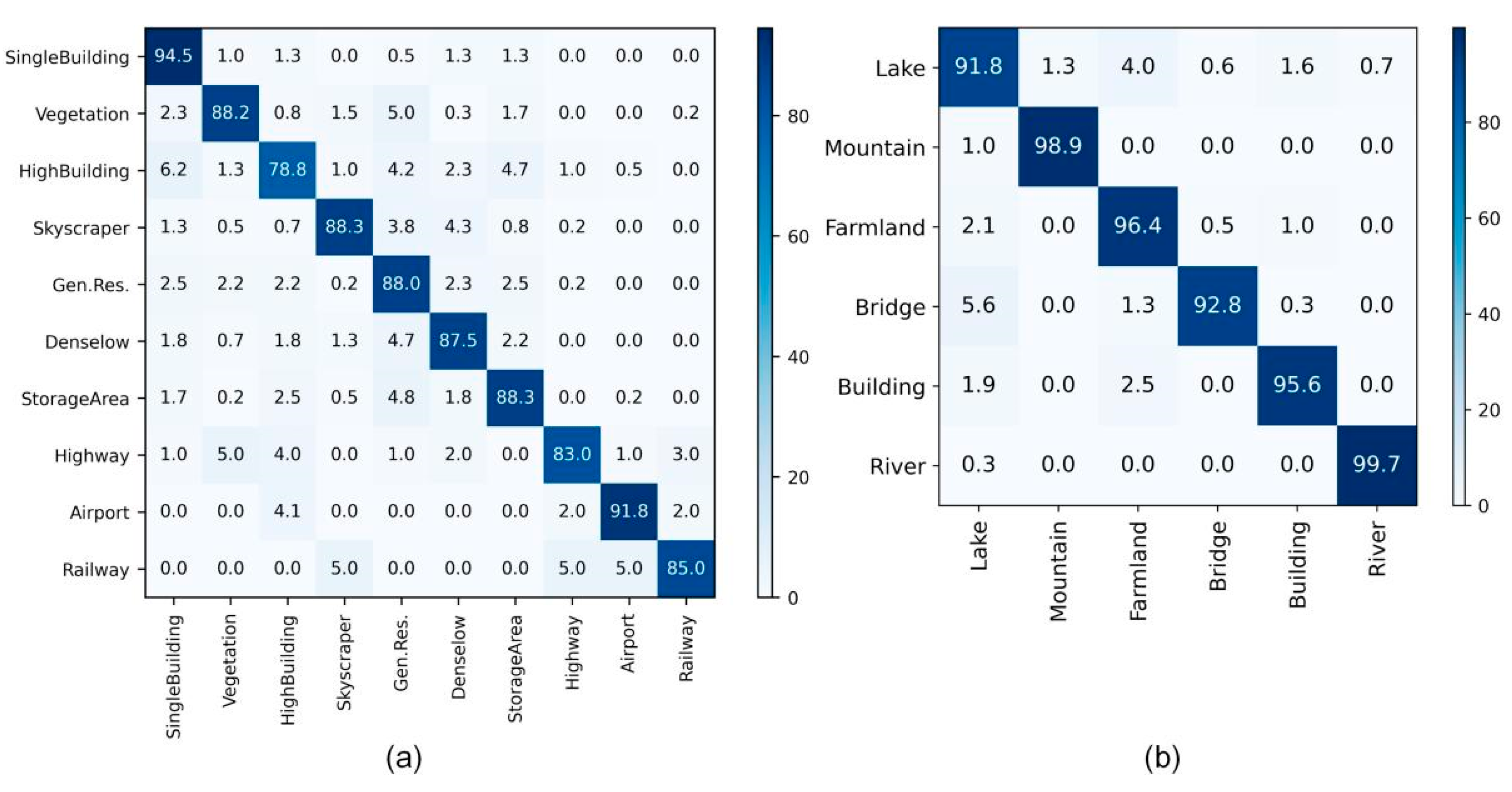
As can be seen from the OpenSARUrban (20%) confusion matrix shown in Figure 9a, the accuracy of the entire test set is 85.43%. High Building category reported the lowest recognition accuracy, and 6.2% were incorrectly identified as Single Building. Urban building areas including Gen.Res, High Building, Single Building, and Denselow showed high misclassifications, as these urban functional areas have similar characteristics. Due to the imbalance of each category, Railway only had 20 test samples with three incorrect classifications.
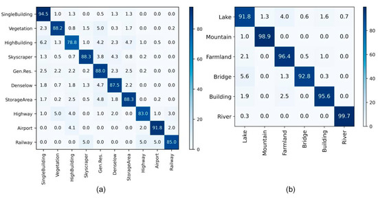
Figure 9.
Confusion matrix of fine-tuned results: (a) on OpenSARUrban with 20% training proportion; (b) on WHU-SAR6 with 20% training proportion.
Figure 9b shows the confusion matrix of fine-tuned results on WHU-SAR6 (20%), the accuracy of the entire test set is 95.83%, with four of the six categories achieving 95% or higher accuracy. Lake and Bridge are the two classes with the highest confusion rates because these two categories both contain water areas.
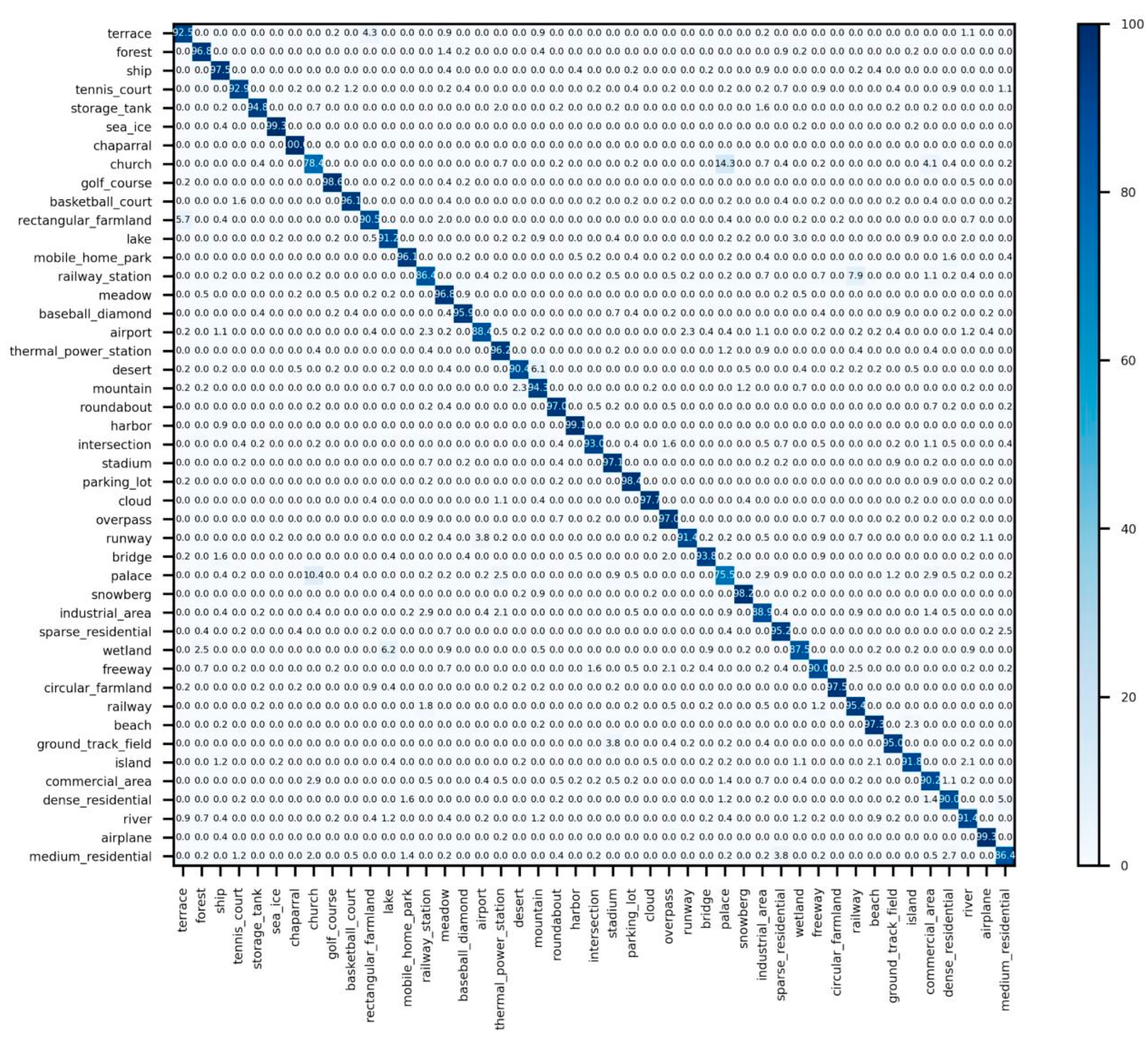
As can be seen from the NWPU-45 (20%) confusion matrix shown in Figure 10, With 38 of the 45 categories achieving 90% or higher accuracy, the accuracy of the entire test set is 93.51%. Churches and palaces are the two classes with the highest confusion rates because the buildings have similar distribution and appearance in these two groups.

Figure 10.
Confusion matrix of fine-tuned results on NWPU-45 20% training proportion.
Figure 11 shows the confusion matrix of fine-tuned results on the AID (50%) dataset. With 26 of the 30 categories reaching 90% or higher accuracy and 23 categories achieving higher than 95%, the accuracy of the entire test set is 95.78%. Resort and park, and center and square are the categories with the highest confusion rate because the images of resorts and parks have a similar distribution of greenery, while center and square are urban scenes with similar characteristics.
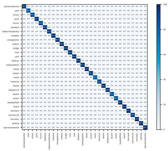
Figure 11.
Confusion matrix of fine-tuned results on AID 50% training proportion.
6. Deployment of Lite-SRL
We applied the Lite-SRL self-supervised algorithm to the proposed DHP distributed training system. The flowchart of deployment is shown in Figure 12.
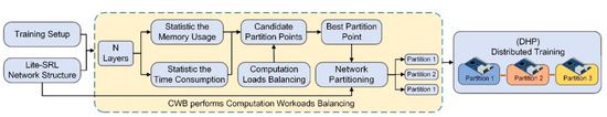
Figure 12.
The flowchart of Lite-SRL’s deployment corresponds to the content in the following. N-Layers corresponds to Figure 13a; Statistic the Memory Usage corresponds to Figure 13b; Statistic the Time Consumption corresponds to Figure 13c; Candidate Partition Points corresponds to Figure 14a; Best Partition Point corresponds to Figure 14b.
6.1. Computation Workload Balancing
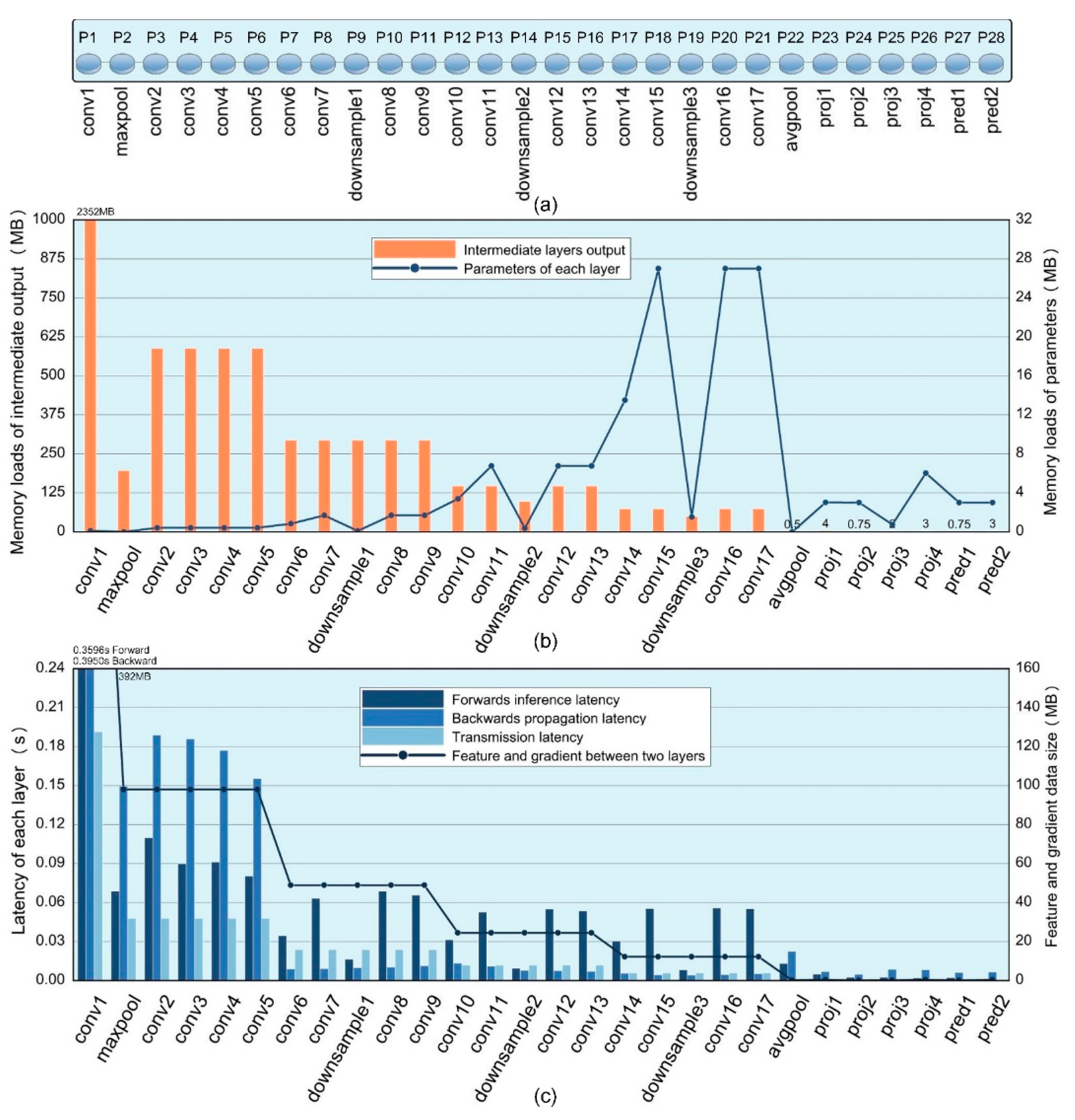
As shown in Figure 13a, CWB figured out all partitionable points over the given Lite-SRL Network structure. CWB requires the following training setup information: (i) the training batch size, (ii) the type of optimizer being used, and (iii) the data exchange rate between TX2 devices to calculate the figures required for workload balancing. In the experiment, the batch is set to 64 and used SGD optimizer with momentum for training. The rate of data transmission between TX2 is simulated by the Linux traffic control tool. According to the partition points and the above setup information, CWB statistic the memory usage and the time consumption of each layer when training on TX2.

Figure 13.
Data collected by CWB. (a) Partitionable layers contained in the Lite-SRL network structure, corresponding to 28 partitionable points . (b) CWB calculated the memory workload occupied by each network layer during the training process, including the intermediate variables and network parameters for each layer. (c) CWB measured time consumption, including inference latency and backward propagation latency of each layer when trained on TX2, together with the data transmission latency between TX2. The transmission latency was derived from the gradient data size between two layers and the inter-device transfer rate.
In experiments we uniformly use the float32 format data type, one data occupies 4 bytes of memory. CWB first performed memory workload balancing and computed the candidate partition points using the data shown in Figure 13b, the theoretical memory usage for all intermediate values during training is 7599.7 MB. Based on experience, each TX2 can achieve a preferable working state when allocating about 3 GB memory of computation, so it requires 3 TX2s to collaborate the training process of one mini-batch. The two sets of candidate partition points calculated by CWB are and , satisfying that the training of each partition can be carried out on a single TX2, the rest of the partition points have been screened out. CWB then performed time equalization utilizing the data in shown Figure 13c, by accumulating the forward and backward latency of individual layers under different candidate partition points, to obtain the running time of each TX2 node during a training batch.
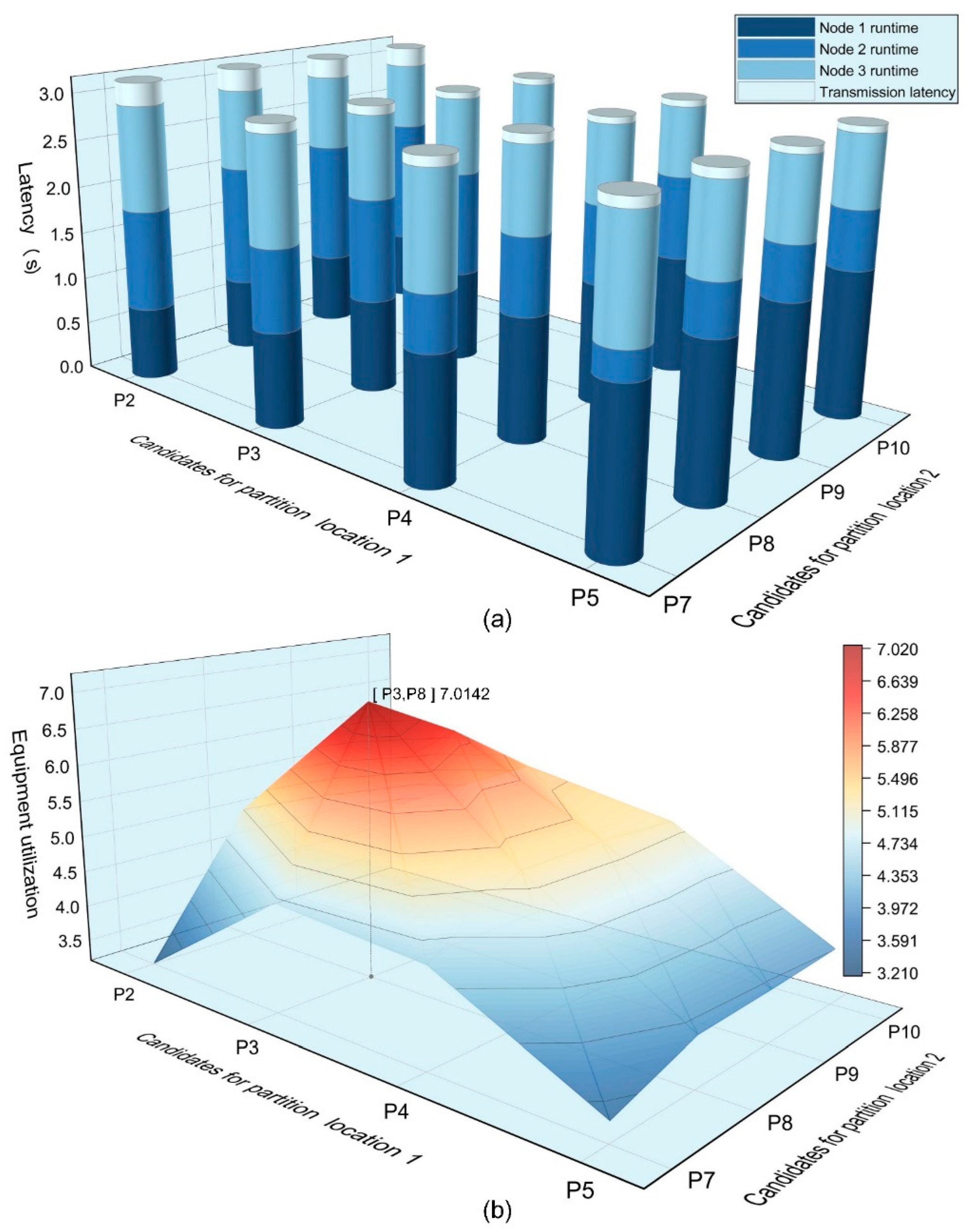
As shown in Figure 14, CWB used the equipment utilization index to find the optimal partition point among the candidate partition points. Figure 14a shows the runtime proportion of each node under candidate partition points, the transmission latency varies depending on different combinations of partition points. In Figure 14b CWB found the partition point combination with the highest equipment utilization [p3, p8], representing the optimal partition points. For the given Lite-SRL network structure and training settings, CWB partitioned it into the following three parts: partition 1 , partition 2 , partition 3 .
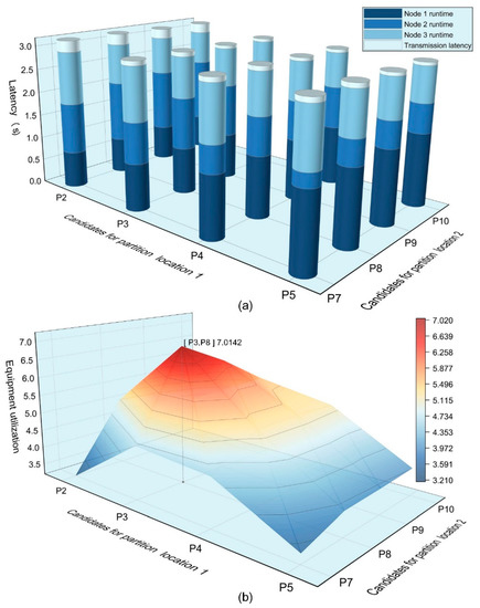
Figure 14.
CWB calculates the optimal partition points. Two sets of candidate partition points are and , the rest of the partition points have been screened out as they cannot satisfy the memory allocation requirements. (a) Runtime proportion of each node under candidate partition points. (b) Using Equation (9) to calculate equipment utilization evaluation indices under candidate partition points.
6.2. Distributed Training with Higher Efficiency
We used six TX2 nodes to compose an on-board computation platform and tested the proposed distributed training baseline along with the improved dynamic chain system. In our on-board distributed training baseline experiments, six nodes formed a two-chain hybrid parallel training according to Figure 4b. After the workload balancing, we allocated the training of three network partitions to TX2 nodes on each chain. In dynamic chain system experiments, three nodes are responsible for the computation of partition 1, two for the computation of partition 2, and one for the computation of partition 3 of the model, as shown in Figure 4b. The two distributed training methods were performed 1000 iterations each, the distributed training system performed parameter aggregation every 100 iterations and updated the model parameters in each node using the aggregated parameters. Here one iteration referred to the completion of one mini-batch’s forward and backward propagation.
As shown in Table 5 and Table 6, the average runtime of executing one iteration in the baseline is 3572 s, while the average time in dynamic chain system is 2750 s.
Table 5.
Distributed training baseline.
Table 6.
Improved dynamic chain system.
The baseline used 6 nodes to complete 1000 iterations of training in 3572 s, and the 2 chains had each been running for 500 iterations. In comparison, the dynamic chain system used the same nodes to complete 1000 iterations of training in 2750 s. With the scheduling of the communication module, the system can be viewed as containing 3 chains; the nodes responsible for the first and second partitions end up with different running iterations, and node 6 completes 1000 iterations. Dynamic chain system improved training efficiency by 23.01% over the baseline without compromising training accuracy.
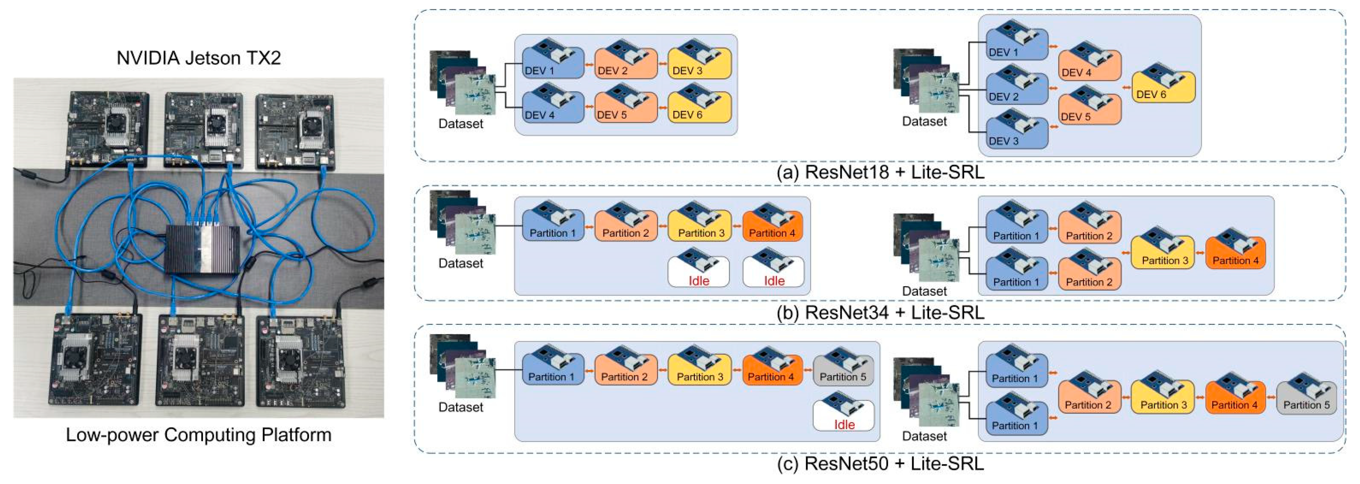
The experimental platform is shown in Figure 15. Our distributed system consists of six nodes, thus allowing flexible distributed training. More chains can be constituted when the calculation demand is low, and more nodes can be invoked to join the training when the calculation demand is high. The proposed Lite-SRL with ResNet-18 as backbone can be completed using 3 TX2 nodes, the baseline and dynamic chain are shown in Figure 15a. When more complex networks need to be trained, it can be achieved by invoking more nodes to join the training, which manifests the advantage of distributed multi-nodes. To this end, we conducted additional experiments. We use the Lite-SRL algorithm, replacing more complex backbone structure as detailed in the following.
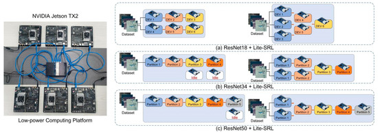
Figure 15.
The left side is the illustration of baseline and the right side is the illustration of dynamic chain system. (a) Lite-SRL with ResNet-18 as encoder; three nodes are required to complete the training of a mini-batch, baseline uses six nodes to form two chains, and dynamic can form three chains. (b) Lite-SRL with ResNet-34 as encoder; four nodes are required to complete the training of a mini-batch. Baseline forms one chain with two nodes idle, while the dynamic chain system can schedule all nodes for training. (c) Lite-SRL with ResNet-50 as encoder, five nodes are required to complete the training of a mini-batch. Baseline forms one chain with 1 node idle, while the dynamic chain system can schedule all nodes for training.
The time consumption of DHP under different training computations is shown in Table 7. The dynamic link system can avoid node idleness and, thus, improve the efficiency of training. Furthermore, through this experiment, we demonstrate the potential of our distributed training system, which can be applied to a wider range of neural network training tasks.
Table 7.
Distributed Training Time Consumption, corresponding to the illustration in Figure 15.
7. Conclusions
In this article, we propose a self-supervised algorithm Lite-SRL for the scene classification task. Our algorithm has clear advantages in terms of overall accuracy, number of parameters, memory consumption, and training latency. We demonstrate that self-supervised algorithms can effectively alleviate the shortage of remote sensing labeled data. Taking the experimental results on NWPU-45 dataset as an example, with training proportions of 10% and 20%, which require few labeled data to predict a large number of test samples, we achieve 92.77% and 93.51% accuracy with a simple network structure after self-supervised pre-training. Previous RSSC studies usually require more complex structures and multiple tricks to achieve such classification accuracies. Meanwhile, our algorithm has far better performance than other methods under 10% training proportion, proving that Lite-SRL’s self-supervised training provides an effective feature extractor.
We exploit the advantage of self-supervised learning by training on satellites. The integration of CWB and DHP enables training neural networks under limited on-board resources. In addition, we add a communication scheduler module to the DHP framework to improve the training speed on top of the baseline. On the experimental computing platform, we successfully transplant Lite-SRL and verify the effectiveness of proposed on-board distributed training modules.
We believe that on-board self-supervised distributed training can facilitate the development of on-board data processing techniques. Not only for RSSC task, but also other tasks in remote sensing such as remote sensing image segmentation [59], target detection [10], etc., can utilize this working paradigm. Our proposed distributed training modules provide strong adaptability, other types of deep learning algorithms can also be deployed in the distributed training framework, making it possible to enhance the intelligence in remote sensing applications.
The next step of our work will be as follows:
- We will design a dedicated lightweight feature extractor in the self-supervised structure to further reduce the memory computation;
- We will explore techniques such as gradient compression, network pruning, etc., to further improve distributed training efficiency;
- We will explore hardware acceleration solutions for onboard distributed training;
- We expect to add more remote sensing observation missions to on-board distributed self-supervised training applications.
Author Contributions
Conceptualization, X.X. and Y.L.; methodology, X.X. and C.L.; software, X.X. and C.L.; investigation, X.X.; resources, X.X.; data curation, X.X. and C.L.; writing—original draft preparation, X.X. and Y.L.; writing—review and editing, X.X. and Y.L.; visualization, X.X.; funding acquisition, Y.L. All authors have read and agreed to the published version of the manuscript.
Funding
This research received no external funding.
Data Availability Statement
No new data were created or analyzed in this study. Data sharing is not applicable to this article.
Conflicts of Interest
The authors declare no conflict of interest.
Appendix A
As shown in Table A1, we list all the abbreviations and their corresponding full names in this article.
Table A1.
The abbreviations and corresponding full names, organized in alphabetical order.
Table A1.
The abbreviations and corresponding full names, organized in alphabetical order.
| Abbreviation | Full Name |
|---|---|
| AID | Aerial Image Dataset |
| BN | Batch Normalization |
| BYOL | Bootstrap Your Own Latent |
| CNN | Convolution Neural Network |
| CWB | Computation workload Balancing module |
| MG-CAP | Multi-Granularity Canonical Appearance Pools |
| MLP | Multi-Layer Perceptron |
| MoCo | Momentum Contrast for Visual Representation Learning |
| MTL | Multitask Learning |
| NWPU-45 | NWPU-Resisc45 Dataset |
| DHP | Distributed Hybrid Parallelism Training Framework |
| Lite-SRL | Lightweight Self-supervised Representation Learning algorithm |
| ReLU | Rectified Linear Unit |
| RSIs | Remote Sensing Images |
| RSSC | Remote Sensing Scene Classification |
| SGD | Stochastic Gradient Descent |
| SimCLR | Simple Framework For Contrastive Learning |
| Simsiam | Simple Siamese Representation Learning |
| SwAV | Unsupervised Learning By Contrasting Cluster Assignments |
| t-SNE | T-Distributed Stochastic Neighbor Embedding |
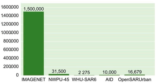
Figure A1.
The total images number of RSSC datasets, i.e., OpenSARUrban [14], WHU-SAR6 [11], NWPU-Resisc45 [3], AID [15] compared with natural image datasets, i.e., ImageNet.
Figure A1.
The total images number of RSSC datasets, i.e., OpenSARUrban [14], WHU-SAR6 [11], NWPU-Resisc45 [3], AID [15] compared with natural image datasets, i.e., ImageNet.
References
- Hu, F.; Xia, G.-S.; Hu, J.; Zhang, L. Transferring Deep Convolutional Neural Networks for the Scene Classification of High-Resolution Remote Sensing Imagery. Remote Sens. 2015, 7, 14680–14707. [Google Scholar] [CrossRef] [Green Version]
- Ni, K.; Liu, P.; Wang, P. Compact Global-Local Convolutional Network with Multifeature Fusion and Learning for Scene Classification in Synthetic Aperture Radar Imagery. IEEE J. Sel. Top. Appl. Earth Obs. Remote Sens. 2021, 14, 7284–7296. [Google Scholar] [CrossRef]
- Cheng, G.; Han, J.; Lu, X. Remote Sensing Image Scene Classification: Benchmark and State of the Art. Proc. IEEE 2017, 105, 1865–1883. [Google Scholar] [CrossRef] [Green Version]
- Xu, X.; Zhang, X.; Zhang, T. Multi-Scale SAR Ship Classification with Convolutional Neural Network. In Proceedings of the IEEE International Geoscience and Remote Sensing Symposium (IGARSS), Online Event, 11–16 July 2021; pp. 4284–4287. [Google Scholar]
- Lu, X.; Sun, X.; Diao, W.; Feng, Y.; Wang, P.; Fu, K. LIL: Lightweight Incremental Learning Approach through Feature Transfer for Remote Sensing Image Scene Classification. IEEE Trans. Geosci. Remote Sens. 2022, 60, 5611320. [Google Scholar] [CrossRef]
- Zhang, T.; Zhang, X. Squeeze-And-Excitation Laplacian Pyramid Network with Dual-Polarization Feature Fusion for Ship Classification in SAR Images. IEEE Geosci. Remote Sens. Lett. 2022, 19, 4019905. [Google Scholar] [CrossRef]
- Gu, Y.; Wang, Y.; Li, Y. A Survey on Deep Learning-Driven Remote Sensing Image Scene Understanding: Scene Classification, Scene Retrieval and Scene-Guided Object Detection. Appl. Sci. 2019, 9, 2110. [Google Scholar] [CrossRef] [Green Version]
- Zhang, T.; Zhang, X.; Ke, X.; Liu, C.; Xu, X. HOG-ShipCLSNet: A Novel Deep Learning Network with HOG Feature Fusion for SAR Ship Classification. IEEE Trans. Geosci. Remote Sens. 2022, 60, 5210322. [Google Scholar] [CrossRef]
- Liao, N.; Datcu, M.; Zhang, Z.; Guo, W.; Zhao, J.; Yu, W. Analyzing the Separability of SAR Classification Dataset in Open Set Conditions. IEEE J. Sel. Top. Appl. Earth Obs. Remote Sens. 2021, 14, 7895–7910. [Google Scholar] [CrossRef]
- Zhang, T.; Zhang, X.; Shi, J.; Wei, S. HyperLi-Net: A Hyper-Light Deep Learning Network for High-Accurate and High-Speed Ship Detection from Synthetic Aperture Radar Imagery. ISPRS J. Photogramm. Remote Sens. 2020, 167, 123–153. [Google Scholar] [CrossRef]
- Su, B.; Liu, J.; Su, X.; Luo, B.; Wang, Q. CFCANet: A Complete Frequency Channel Attention Network for SAR Image Scene Classification. IEEE J. Sel. Top. Appl. Earth Obs. Remote Sens. 2021, 14, 11750–11763. [Google Scholar] [CrossRef]
- Zhang, T.; Zhang, X. A Polarization Fusion Network with Geometric Feature Embedding for SAR Ship Classification. Pattern Recognit. 2022, 123, 108365. [Google Scholar] [CrossRef]
- Dumitru, C.O.; Schwarz, G.; Datcu, M. SAR Image Land Cover Datasets for Classification Benchmarking of Temporal Changes. IEEE J. Sel. Top. Appl. Earth Obs. Remote Sens. 2018, 11, 1571–1592. [Google Scholar] [CrossRef]
- Zhao, J.; Zhang, Z.; Yao, W.; Datcu, M.; Xiong, H.; Yu, W. OpenSARUrban: A Sentinel-1 SAR Image Dataset for Urban Interpretation. IEEE J. Sel. Top. Appl. Earth Obs. Remote Sens. 2020, 13, 187–203. [Google Scholar] [CrossRef]
- Xia, G.-S.; Hu, J.; Hu, F.; Shi, B.; Bai, X.; Zhong, Y.; Zhang, L.; Lu, X. AID: A Benchmark Data Set for Performance Evaluation of Aerial Scene Classification. IEEE Trans. Geosci. Remote Sens. 2017, 55, 3965–3981. [Google Scholar] [CrossRef] [Green Version]
- Deng, J.; Dong, W.; Socher, R.; Li, L.-J.; Li, K.; Fei-Fei, L. ImageNet: A large-scale hierarchical image database. In Proceedings of the 2009 IEEE Conference on Computer Vision and Pattern Recognition (CVPR), Miami, FL, USA, 20–25 June 2009; pp. 248–255. [Google Scholar]
- Zhang, T.; Zhang, X. A Full-Level Context Squeeze-And-Excitation ROI Extractor for SAR Ship Instance Segmentation. IEEE Geosci. Remote Sens. Lett. 2022, 19, 4506705. [Google Scholar] [CrossRef]
- Kolesnikov, A.; Zhai, X.; Beyer, L. Revisiting self-supervised visual representation learning. In Proceedings of the IEEE/CVF Conference on Computer Vision and Pattern Recognition (CVPR), Long Beach, CA, USA, 15–20 June 2019; pp. 1920–1929. [Google Scholar]
- Noroozi, M.; Favaro, P. Unsupervised learning of visual representations by solving jigsaw puzzles. In European Conference on Computer Vision; Springer: Cham, Switzerland, 2016; pp. 69–84. [Google Scholar]
- Stojnic, V.; Risojevic, V. Self-supervised learning of remote sensing scene representations using contrastive multiview coding. In Proceedings of the IEEE/CVF Conference on Computer Vision and Pattern Recognition (CVPR), Nashville, TN, USA, 19–25 June 2021; pp. 1182–1191. [Google Scholar]
- Zhang, T.; Zhang, X.; Shi, J.; Wei, S.; Wang, J.; Li, J.; Su, H.; Zhou, Y. Balance Scene Learning Mechanism for Offshore and Inshore Ship Detection in SAR Images. IEEE Geosci. Remote Sens. Lett. 2022, 19, 4004905. [Google Scholar] [CrossRef]
- Chen, T.; Kornblith, S.; Norouzi, M.; Hinton, G. A simple framework for contrastive learning of visual representations. In Proceedings of the International Conference on Machine Learning, Vienna, Austria, 12–18 July 2020; Volume 119, pp. 1597–1607. [Google Scholar]
- Ayush, K.; Uzkent, B.; Meng, C.; Tanmay, K.; Burke, M.; Lobell, D.; Ermon, S. Geography-aware self-supervised learning. In Proceedings of the IEEE/CVF International Conference on Computer Vision (ICCV), Montreal, QC, Canada, 10–17 October 2021; pp. 10181–10190. [Google Scholar]
- Franklin, D. NVIDIA Developer Blog: NVIDIA Jetson TX2 Delivers Twice the Intelligence to the Edge. Available online: https://devblogs.nvidia.com/jetson-tx2-delivers-twice-intelligence-edge/ (accessed on 13 April 2022).
- Xu, X.; Zhang, X.; Zhang, T. Lite-YOLOv5: A Lightweight Deep Learning Detector for On-Board Ship Detection in Large-Scene Sentinel-1 SAR Images. Remote Sens. 2022, 14, 1018. [Google Scholar] [CrossRef]
- Aitech’s S-A1760 Venus™ Brings NVIDIA-Based AI Supercomputing to Next Generation Space Applications: Radiation-CharActerized COTS System Qualified for Use in Small Sat Clusters and Short-Duration Spaceflights. Available online: https://aitechsystems.com/aitechs-s-a1760-venus-brings-nvidia-based-ai-supercomputing-to-next-generation-space-applications/ (accessed on 13 April 2022).
- Paszke, A.; Gross, S.; Massa, F.; Lerer, A.; Bradbury, J.; Chanan, G.; Killeen, T.; Lin, Z.; Gimelshein, N.; Antiga, L. Pytorch: An imperative style, high-performance deep learning library. Adv. Neural Inf. Processing Syst. 2019, 32, 8026–8037. [Google Scholar]
- Abadi, M.; Barham, P.; Chen, J.; Chen, Z.; Davis, A.; Dean, J.; Devin, M.; Ghemawat, S.; Irving, G.; Isard, M. Tensorflow: A system for large-scale machine learning. In Proceedings of the 12th {USENIX} Symposium on Operating Systems Design and Implementation ({OSDI} 16), Savannah, GA, USA, 2–4 November 2016; pp. 265–283. [Google Scholar]
- Jia, Y.; Shelhamer, E.; Donahue, J.; Karayev, S.; Long, J.; Girshick, R.; Guadarrama, S.; Darrell, T. Caffe: Convolutional architecture for fast feature embedding. In Proceedings of the 22nd ACM International Conference on Multimedia, Orlando, FL, USA, 3–7 November 2014; pp. 675–678. [Google Scholar]
- Shazeer, N.; Cheng, Y.; Parmar, N.; Tran, D.; Vaswani, A.; Koanantakool, P.; Hawkins, P.; Lee, H.; Hong, M.; Young, C.; et al. Mesh-tensorflow: Deep learning for supercomputers. arXiv 2018, arXiv:1811.02084. [Google Scholar]
- Onoufriou, G.; Bickerton, R.; Pearson, S.; Leontidis, G. Nemesyst: A hybrid parallelism deep learning-based framework applied for internet of things enabled food retailing refrigeration systems. Comput. Ind. 2019, 113, 103133. [Google Scholar] [CrossRef] [Green Version]
- Grill, J.-B.; Strub, F.; Altché, F.; Tallec, C.; Richemond, P.H.; Buchatskaya, E.; Doersch, C.; Pires, B.A.; Guo, Z.D.; Azar, M.G. Bootstrap your own latent: A new approach to self-supervised learning. arXiv 2020, arXiv:2006.07733. [Google Scholar]
- Chen, X.; He, K. Exploring simple siamese representation learning. In Proceedings of the IEEE/CVF Conference on Computer Vision and Pattern Recognition (CVPR), Nashville, TN, USA, 19–25 June 2021; pp. 15750–15758. [Google Scholar]
- Li, X.; Shi, D.; Diao, X.; Xu, H. SCL-MLNet: Boosting Few-Shot Remote Sensing Scene Classification via Self-Supervised Contrastive Learning. IEEE Trans. Geosci. Remote Sens. 2022, 60, 5801112. [Google Scholar] [CrossRef]
- Li, Y.; Shao, Z.; Huang, X.; Cai, B.; Peng, S. Meta-FSEO: A Meta-Learning Fast Adaptation with Self-Supervised Embedding Optimization for Few-Shot Remote Sensing Scene Classification. Remote Sens. 2021, 13, 2776. [Google Scholar] [CrossRef]
- Tao, C.; Qi, J.; Lu, W.; Wang, H.; Li, H. Remote Sensing Image Scene Classification With Self-Supervised Paradigm Under Limited Labeled Samples. IEEE Geosci. Remote Sens. Lett. 2022, 19, 8004005. [Google Scholar] [CrossRef]
- Kang, J.; Fernandez-Beltran, R.; Duan, P.; Liu, S.; Plaza, A.J. Deep Unsupervised Embedding for Remotely Sensed Images Based on Spatially Augmented Momentum Contrast. IEEE Trans. Geosci. Remote Sens. 2021, 59, 2598–2610. [Google Scholar] [CrossRef]
- Jung, H.; Oh, Y.; Jeong, S.; Lee, C.; Jeon, T. Contrastive Self-Supervised Learning with Smoothed Representation for Remote Sensing. IEEE Geosci. Remote Sens. Lett. 2021, 19, 8010105. [Google Scholar] [CrossRef]
- Zhao, L.; Luo, W.; Liao, Q.; Chen, S.; Wu, J. Hyperspectral Image Classification with Contrastive Self-Supervised Learning under Limited Labeled Samples. IEEE Geosci. Remote Sens. Lett. 2022, 19, 6008205. [Google Scholar] [CrossRef]
- Doersch, C.; Gupta, A.; Efros, A.A. Unsupervised visual representation learning by context prediction. In Proceedings of the IEEE International Conference on Computer Vision (ICCV), Santiago, Chile, 7–13 December 2015; pp. 1422–1430. [Google Scholar]
- Pathak, D.; Krahenbuhl, P.; Donahue, J.; Darrell, T.; Efros, A.A. Context encoders: Feature learning by inpainting. In Proceedings of the IEEE/CVF Conference on Computer Vision and Pattern Recognition (CVPR), Las Vegas, NV, USA, 27–30 June 2016; pp. 2536–2544. [Google Scholar]
- He, K.; Fan, H.; Wu, Y.; Xie, S.; Girshick, R. Momentum contrast for unsupervised visual representation learning. In Proceedings of the IEEE/CVF Conference on Computer Vision and Pattern Recognition (CVPR), Seattle, WA, USA, 13–19 June 2020; pp. 9729–9738. [Google Scholar]
- Chen, X.; Fan, H.; Girshick, R.; He, K. Improved baselines with momentum contrastive learning. arXiv 2020, arXiv:2003.04297. [Google Scholar]
- Caron, M.; Misra, I.; Mairal, J.; Goyal, P.; Bojanowski, P.; Joulin, A. Unsupervised learning of visual features by contrasting cluster assignments. arXiv 2020, arXiv:2006.09882. [Google Scholar]
- Krizhevsky, A.; Sutskever, I.; Hinton, G.E. Imagenet classification with deep convolutional neural networks. Adv. Neural Inf. Process. Syst. 2012, 25, 1097–1105. [Google Scholar] [CrossRef]
- Kim, S.; Yu, G.-I.; Park, H.; Cho, S.; Jeong, E.; Ha, H.; Lee, S.; Jeong, J.S.; Chun, B.-G. Parallax: Sparsity-aware data parallel training of deep neural networks. In Proceedings of the Fourteenth EuroSys Conference, Dresden, Germany, 25–28 March 2019; pp. 1–15. [Google Scholar]
- Jia, Z.; Zaharia, M.; Aiken, A. Beyond data and model parallelism for deep neural networks. Proc. Mach. Learn. Syst. 2019, 1, 1–13. [Google Scholar]
- Lee, S.; Kim, J.K.; Zheng, X.; Ho, Q.; Gibson, G.; Xing, P. On Model Parallelization and Scheduling Strategies for Distributed Machine Learning; Carnegie Mellon University: Pittsburgh, PA, USA, 2014; pp. 2834–2842. [Google Scholar]
- Akintoye, S.B.; Han, L.; Zhang, X.; Chen, H.; Zhang, D. A hybrid parallelization approach for distributed and scalable deep learning. arXiv 2021, arXiv:2104.05035. [Google Scholar] [CrossRef]
- Demirci, G.V.; Ferhatosmanoglu, H. Partitioning sparse deep neural networks for scalable training and inference. In Proceedings of the ACM International Conference on Supercomputing, Virtual Event, 14–17 June 2021; pp. 254–265. [Google Scholar]
- Moreno-Alvarez, S.; Haut, J.M.; Paoletti, M.E.; Rico-Gallego, J.A. Heterogeneous model parallelism for deep neural networks. Neuro Comput. 2021, 441, 1–12. [Google Scholar] [CrossRef]
- Das, D.; Avancha, S.; Mudigere, D.; Vaidynathan, K.; Sridharan, S.; Kalamkar, D.; Kaul, B.; Dubey, P. Distributed deep learning using synchronous stochastic gradient descent. arXiv 2016, arXiv:1602.06709. [Google Scholar]
- He, K.; Zhang, X.; Ren, S.; Sun, J. Deep residual learning for image recognition. In Proceedings of the IEEE/CVF Conference on Computer Vision and Pattern Recognition (CVPR), Las Vegas, NV, USA, 27–30 June 2016; pp. 770–778. [Google Scholar]
- Van Hinton, G. Visualizing data using t-SNE. J. Mach. Learn. Res. 2008, 9, 2579–2605. [Google Scholar]
- Cheng, G.; Yang, C.; Yao, X.; Guo, L.; Han, J. When Deep Learning Meets Metric Learning: Remote Sensing Image Scene Classification via Learning Discriminative CNNs. IEEE Trans. Geosci. Remote Sens. 2018, 56, 2811–2821. [Google Scholar] [CrossRef]
- Chen, Z.; Wang, S.; Hou, X.; Shao, L.; Dhabi, A. Recurrent transformer network for remote sensing scene categorisation. In Proceedings of the 2018 British Machine Vision Conference, Newcastle, UK, 3–6 September 2018; Volume 266, p. 0987. [Google Scholar]
- Wang, S.; Guan, Y.; Shao, L. Multi-Granularity Canonical Appearance Pooling for Remote Sensing Scene Classification. IEEE Trans. Image Proces. 2020, 29, 5396–5407. [Google Scholar] [CrossRef] [Green Version]
- Zhao, Z.; Luo, Z.; Li, J.; Chen, C.; Piao, Y. When Self-Supervised Learning Meets Scene Classification: Remote Sensing Scene Classification Based on a Multitask Learning Framework. Remote Sens. 2020, 12, 3276. [Google Scholar] [CrossRef]
- Zhang, T.; Zhang, X. HTC+ for SAR Ship Instance Segmentation. Remote Sens. 2022, 14, 2395. [Google Scholar] [CrossRef]


Publisher’s Note: MDPI stays neutral with regard to jurisdictional claims in published maps and institutional affiliations. |
© 2022 by the authors. Licensee MDPI, Basel, Switzerland. This article is an open access article distributed under the terms and conditions of the Creative Commons Attribution (CC BY) license (https://creativecommons.org/licenses/by/4.0/).