Article

Detection of Irrigated Permanent Grasslands with Sentinel-2 Based on Temporal Patterns of the Leaf Area Index (LAI)

1
1114 UMR INRAE, Avignon University EMMAH, Domaine St. Paul, 84914 Avignon, France
2
Agronomy Department, Faculty of Agriculture, Shabu-Lafia Campus, Nasarawa State University, Keffi 961101, Nigeria
*
Author to whom correspondence should be addressed.
Remote Sens. 2022, 14(13), 3056; https://doi.org/10.3390/rs14133056
Submission received: 18 May 2022 / Revised: 21 June 2022 / Accepted: 22 June 2022 / Published: 25 June 2022

Abstract

:
Conventional methods of crop mapping need ground truth information to train the classifier. Thanks to the frequent acquisition allowed by recent satellite missions (Sentinel 2), we can identify temporal patterns that depend on both phenology and crop management. Some of these patterns are specific to a given crop and thus can be used to map it. Thus, we can substitute ground truth information used in conventional methods with agronomic knowledge. This approach was applied to identify irrigated permanent grasslands (IPG) in the Crau area (Southern France), which play a crucial role in groundwater recharge. The grassland is managed by making three mows during the May–October period, which leads to a specific temporal pattern of leaf area index (LAI). The mowing detection algorithm was designed using the temporal LAI signal derived from Sentinel 2 observations. The algorithm includes some filtering to remove noise in the signal that might lead to false mowing detection. A pixel is considered a grassland if the number of detected mows is greater than 1. A data set covering five years (2016–2020) was used. The detection mowing number was conducted at the pixel level, and then the results were aggregated at the plot level. An evaluation data set including 780 plots was used to assess the performances of the classification. We obtained a Kappa index ranging between 0.94 and 0.99 according to the year. These results were better than other supervised classification methods that include training data sets. The analysis of land-use changes shows that misclassified plots concern grasslands managed less intensively with strong intra-parcel heterogeneity due to irrigation defects or year-round grazing. Time series analysis, therefore, allows us to understand different management practices. Real land-use change in use can be observed, but long time series are needed to confirm the change and remove ambiguities with heterogeneous grasslands.

Graphical Abstract

1. Introduction

According to United Nations [1], water is a scarce resource; thus, its justifiable and judicious use must remain a crucial and fundamental target for sustainable developments across the globe, especially in a world with a constantly increasing populace that directly or indirectly depends on this scarce resource for sustaining their activity and food production system. Undoubtedly, agriculture remains an obvious focal point in water management as the main water user [2], with irrigation accounting at world-scale for about 70% of global freshwater withdrawals [3]. The effect of global changes is anticipated to heighten the issue of water shortage and irrigation needs [4]. Thus, attention is needed on appraisals related to irrigation activities to bolster water resource management, maximize water productivity, and boost agricultural water sustainability [5]. To match water needs and resources, better planning is needed for irrigation activities [6]. One of the key solutions to good irrigation planning is the provision of extensively detailed spatial delineations of croplands under irrigation [7] and the description of irrigation systems and strategies that may lead to various water needs across the year [8]. There is, therefore, a challenge to detect not only the irrigated areas but also the associated production systems.
The classification of irrigated areas is widely discussed in the literature [8]. While the use of medium resolution satellites has allowed the establishment of methodological bases applicable to regional scales, there is a renewed interest in these methods with the Sentinel satellites, which offer both good temporal repeatability (3–5 days) and good spatial resolution (10 m), which is particularly relevant for crop monitoring. Classification methods for irrigated surfaces are generally based on radar data providing a temporal series of surface moisture, data in the optical domain with monitoring of vegetation dynamics, and meteorological data. The use of optical data relative to separate irrigated and non-irrigated areas is based on the green cover dynamic, which displays higher levels when additional water is brought to the crop. Indices based on meteorological data enhance the quality of the classification. In general, these indices are linked to climatic water stress, which allows for a better characterization of irrigation periods [9,10,11]. In addition to the meteorological data, thermal infrared observations enable the implementation of surface energy balance model to infer the evaporative fraction that is found as a relevant classifier [12] complementary to vegetation indices.
Supervised classification is the most common approach with the implementation of different methods such as decision trees, random forest, support vector machine (SVM), or neural network for the most frequently cited. The classifiers are in general based on the remotely sensed quantities and/or the derived indices combining several measurements as spectral indices in the optical domain or the radar polarization ratio. It is difficult to report on the obtained accuracy in general terms, since the pedoclimatic conditions, the spatial domain, and the type irrigated and non-irrigated crop differ considerably from one study to another. For instance, the kappa index ranges between 0.36 [9] and 0.9 [13]. In recent years many studies are based on Sentinel satellite observations [8] using either Sentinel-1 and -2 or both. The combined use of radar Sentinel-1 and optical Sentinel-2 has shown a moderate improvement in classifications [5,13,14] when compared to method based on using Sentinel-2 only. However, supervised classification has some limitations, such as the need to collect training data or to deal with missing data. The latter can be an important issue in the optical domain with the clouds. Therefore, when working over large spatial domains, the selection of cloud-free images can considerably reduce the time series.
An alternative is to use temporal characteristics of the remotely sensed quantities. For instance, in [10], a classification on the temporal characteristics of the vegetation signal such as the maximum and the range of variation of the vegetation index is proposed. For an 18-year period, training can be limited to a wet and dry year, while an excellent overall accuracy was obtained (>0.95). The authors of [5] showed that it is possible to separate irrigation systems between crops and orchards based on the variability of the radar signal and the temporal autocorrelation length of this signal. Several studies [6,10,11,15] show that the consideration of agronomic traits related to phenology and cropping interventions can provide relevant information to characterize irrigated systems. In a broader context, it is found that agronomic features can be extracted from multitemporal remote sensing data [16] and apply to crop mapping as for instance with canola [17] and potatoes [18] with an improved accuracy in comparison to classical supervised classification methods. These encouraging results led us to take profit of the short revisit time of Sentinel-2 satellites to map Irrigated Permanent Grasslands (IPG) using a temporal approach based on the detection of agronomic traits. In the study site (the Crau area in south east France), IPGs were irrigated using flooding techniques, which not only has a strong impact on the regional water budget by consuming a very large amount of water (about 20,000 m3/ha/year [19]) but also provides important externalities such as groundwater recharge. IPG is an interesting case as it provides very clear agronomic traits with several mowing events across the year that can be used for the classification.
The characterisation of grasslands has already been the subject of several studies. The authors of [20] showed that, with a limited number of SPOT images (three in the study), one can separate mown grasslands from grazed grasslands with a kappa = 0.82. In this study, it was also found that LAI is the best indicator to make such a distinction. More recently, the authors of [21] classify grassland use intensity with five rapid eyes images based on the variability of the temporal signal. A similar approach was followed by [22] who used a series of 14 Landsat dates to distinguish six classes of grassland reflecting different management strategies. These results announce the potential of Sentinel-2, which was used to detect mowing events [23,24,25,26,27]. All proposed methods are based on frequent temporal sampling of vegetation index and local minimum detection. The proposed approaches differ in the methods for filtering the vegetation indices time series and the algorithm for detecting local minima associated with mowing. The quality of the results depends on the scale of the work, with overall accuracies of about 70–80% for studies covering large regional territories [24,27] and better than 90% for smaller territories [26]. The difficulties mentioned by these studies concern the variability of management methods, such as the quantities of grass removed during mowing, spatial heterogeneities (e.g., presence of trees), and acquisition dates that are not always optimal for identifying mowing events. The use of radar series that are not impacted by cloud covers is an alternative exploited in [28,29]. However, the rate of detection errors remains significant due to errors that are inherent to the measured quantities and its interaction with other factors as the plant water content. The combination of optical and radar images was implemented in [25]. The authors used a deep learning algorithm and showed that combining radar quantities (coherence and backscattering coefficient) and NDVI is the best option with an F1-score obtained at regional scale of 0.88. It should be noted that these characterisations are performed on known grassland areas and are not used for the classification of grassland areas. The originality of the present study was then to explore the capabilities of mowing event detection to map IPG and non-irrigated grassland (NIG).
The goal of the study was to develop a classification method to map IPG in South-East France. The approach was developed in the context of the Crau area in Southern France in the Mediterranean. IPG are both an emblematic crop of the areas and plays an important role in the superficial aquifer water budget [19]. In this paper, we develop a mowing event algorithm that is able to minimise false mowing event detection and account for temporal sampling of Sentinel-2 data that may present missing observation dates during mowing periods. The classification performance was compared to the traditional classification method made directly on vegetation indices time series and the THEIA product, which is an operational product implemented over France.

2. Materials and Methods
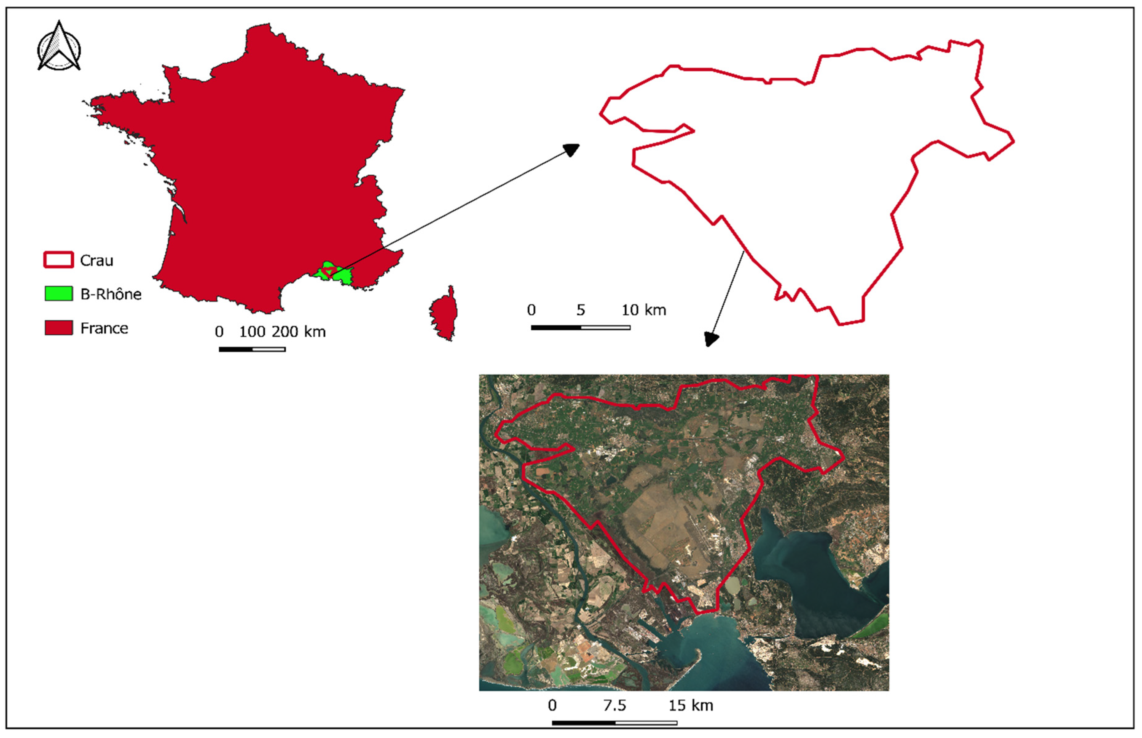
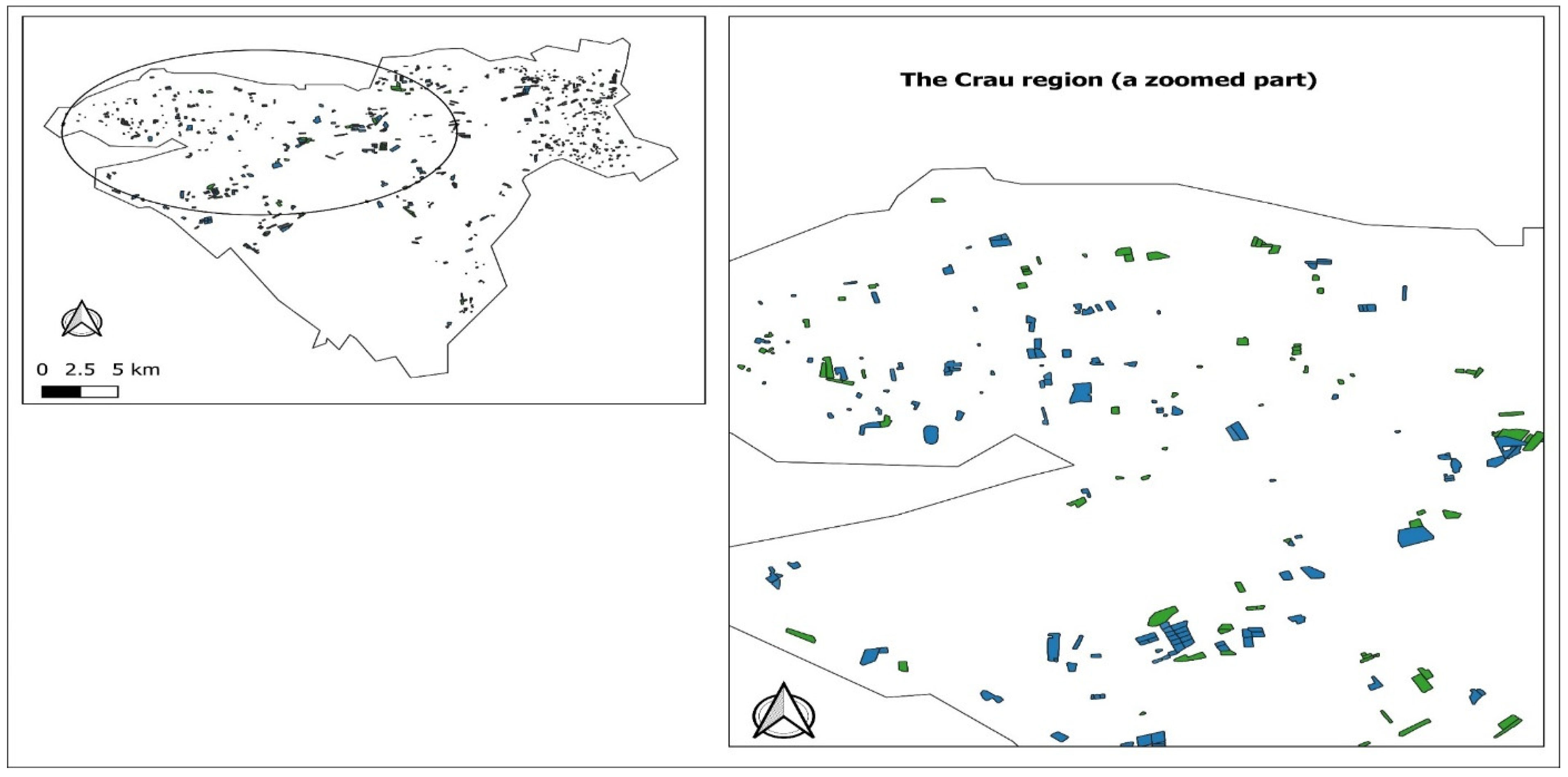
2.1. The Study Site

The Crau area (Figure 1) is located at 43°38′N, 5°00′E (5 m a.s.l) near the Rhône delta in Southern France, which covers a surface area of 540 to 600 km2. The climate of the Crau area is Mediterranean with an average annual rainfall of 600 mm (non-uniform) and a potential evapotranspiration of 1100 mm. Mean air temperature of about 7–8 °C (in winter) and 24 °C (in summer) [23,30,31]. The Crau area is characterised by native shallow soils of about 60–80 cm with 90% stones, consequently rendering its water retention very low. Soils irrigated using flooding technics present a loamy surface soil layer thanks to sediments transported via irrigation water with a layer depth that can reach 60 cm depending on the length of the irrigation period [23]. IPGs are the most predominant irrigated crops in the Crau area [19,23] with a coverage of about 13,000 ha (23%), as depicted in Figure 1 (the dark green plots). The irrigation practice of permanent grasslands in the Crau area is more than 4 centuries old, which can be dated back to the 16th century [30]. The common practice mostly remains the same, which involves the use of gravity (flood) for irrigation, on areas specifically dedicated to hay production and rearing of sheep. The water used for flooding irrigation contributes to more than 75% of the groundwater table. This ground water table is used for the irrigation of intensive orchard and market garden productions and domestic and industrial purposes to roughly 280,000 people around the southern part of the area [23,30]. The duration for irrigation in a year extends to about seven months [19] from March to September. IPG management is regulated by the selling label “foin de Crau”, the first COP (Certified Origin Product) in France leading to standardised management with three or four grass mowings from 1 May to the end of October and sheep grazing in winter. In general, grass fields are irrigated optimally to cover the water needs, but in some places and some years, the access to water might be critical, thus leading to reduced grass productivity and skipping a mowing operation. Some farmers do not follow label rules (for example, when they breed animals all year round), which leads to a different spatial and temporal dynamics of the vegetation cover than the one obtained with the recommended cultivation practices, which are dominant on the territory. The grass fields are in general homogeneous but heterogeneities in vegetation cover were found at the field boarder or within the field when surface levelling is not satisfactory, generating heterogeneities in the water supply. Therefore, if a dominant grass development temporal pattern is expected and then used to identify grassland areas, the mentioned variation can interfere with the classification process.

2.2. Data Used

2.2.1. Field Survey

A field survey was conducted to identify crop type and irrigation over a total of 809 plots (all plots were greater than 1 ha) by a visit during the 2016–2020 periods. During the visit, surveyed plots were identified and observed crop were reported in the plot map established over the entire area. Irrigated permanent grasslands (IPG) consisted of 391 plots and not irrigated grasslands (NIGs) comprise 418 plots. In addition, aerial photographs were used to verify management features such as soil levelling, land-use change, or grazing. For that purpose, we used Google Earth images acquired during the 2015–2021 period together with the IGN (the French National Geography Institute) 2020 flight campaign. Plot boundaries were drawn in 2012 throughout the Crau area, leading to 18,058 polygons. The map was initiated with the cadastre, which we then corrected manually to delimit homogeneous spatial entities in terms of their use hereafter referred to as plot. The resulting SIG layer was then used to aggregate classification results produced at pixel scale over plot’s polygons

2.2.2. Satellite Data

Time series of Sentinel-2 of level 2A optical images were used for this study, which were collected from both Sentinel-2A and Sentinel-2B for all dates from 2016 to 2020. We used the images distributed by the French land data open-source service centre (https://www.theia-land.fr/, accessed on 17 May 2022), which also proposed cloud masks that were used to remove pixels affected by clouds. The number of remaining dates during the considered period (15 March to 30 October) is provided in Table 1. As Sentinel 2B satellite was operational during 2017, we obtained a lower number of dates in 2016 and 2017. At the pixel level, the number of available dates varied due to occurrence of clouds, which was not homogeneous within the studied area.
The BVNET algorithm using bands 3, 4, and 8 was used. The algorithm calculates biophysical canopy variables such as Leaf area Index (LAI). Due to its robustness, especially on homogeneous canopies such as grasslands, the algorithm has been integrated in the S2toolbox developed by European Space Agency. It is based on neural network trained on simulated spectral reflectance using a radiative transfer model [32]. Temporal profiles of LAI were then established for every 10 m pixel.

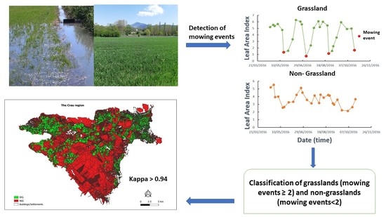
2.3. Developed Irrigated Permanent Grassland Detection Algorithm

The specificity of irrigated grasslands is that they present several mowing–vegetation growth cycles during the year. To detect a grassland, we can also rely on the level of LAI, which is generally high (LAI > 4) when the vegetation is well developed, and the growth rate after a cut is specific to the grassland. For example, in the study area, it takes 30 to 50 days after a mow to return to a vegetation development comparable to that before the mow. Although these characteristics specific to irrigated grassland should make it relatively easy to identify them with temporal sampling such as that offered by the Sentinel-2 mission, we were confronted in the time series with LAI variations linked to atmospheric corrections that may generate temporal patterns of LAI leading to confusion with grassland mowing events. In addition, the presence of clouds during the mowing periods reduced the time sampling of LAI and prevents a clear detection of a mowing event.
As in [23,24,26,27], the detection algorithms of mowing events developed in the study are based on a sharp reduction in vegetation amount followed by significant vegetation developments during the following 45 days. To monitor the development of vegetation, we used the LAI estimated from Sentinel-2. If this quantity has not been used in previous mowing event detection studies that rely on NDVI or NDII [23,24,26,27], the main reason for this choice comes from the nature of the quantity, which is a characteristic of plant cover and can, therefore, be directly linked to agronomic knowledge and crop model outputs. This is important for the design of algorithms characterising agronomic traits, their parameterisation, and their generalisation to include prior information from agronomic knowledge. Moreover, it has be shown that LAI is more sensitive to variations in well-developed vegetation, while conventional vegetation indices tend to saturate more easily [29]. The disadvantage is that the computed LAIs are more sensitive to atmospheric corrections as we no longer have the normalization of measurements made on classical vegetation indices such as NDVI. Moreover, on some surface types, the LAI inversion algorithm may fail. For example, we found very high and variable LAI values on greenhouses with a non-negligible risk of confusion with grasslands.
To detect an irrigated grassland, we made the following main assumptions:
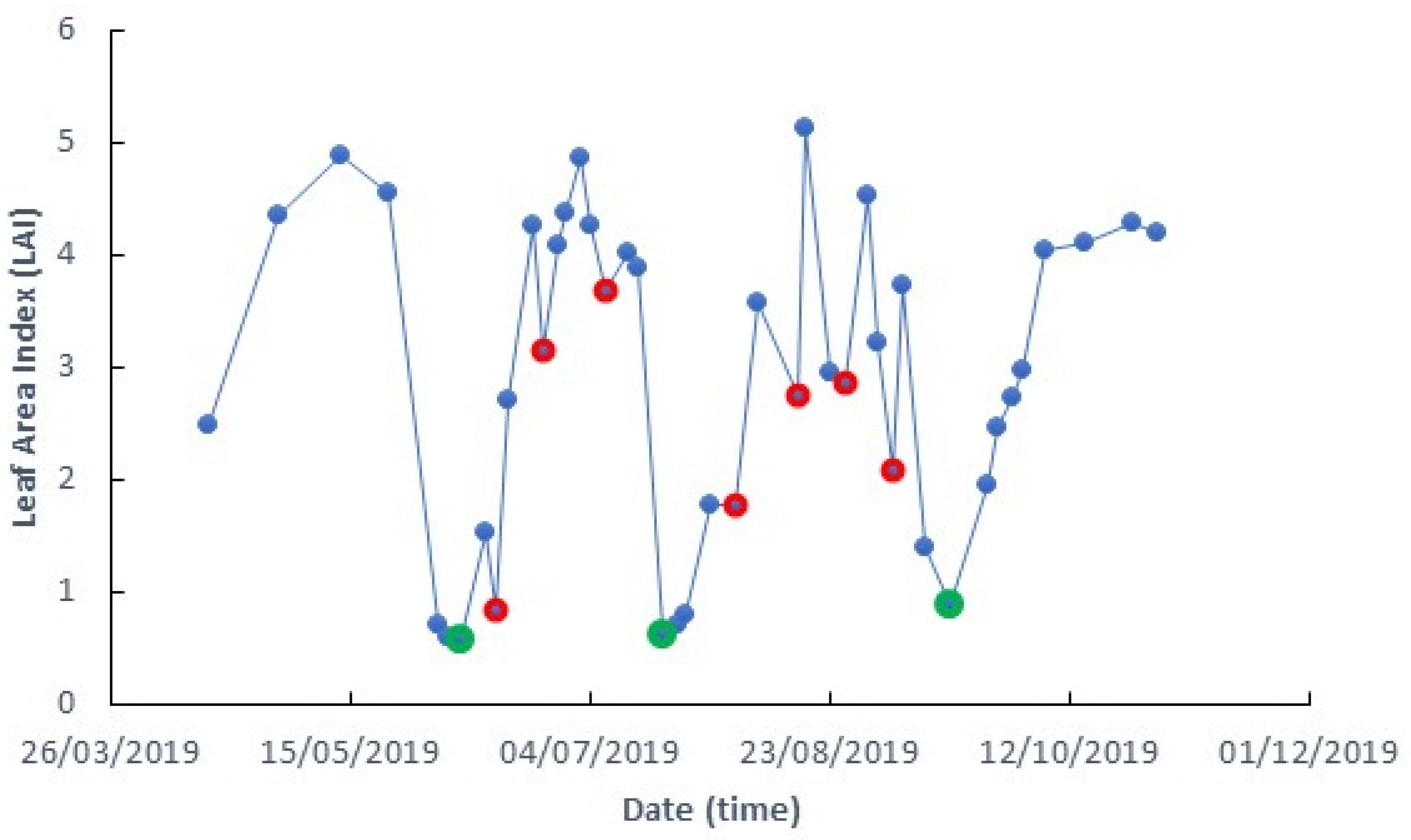
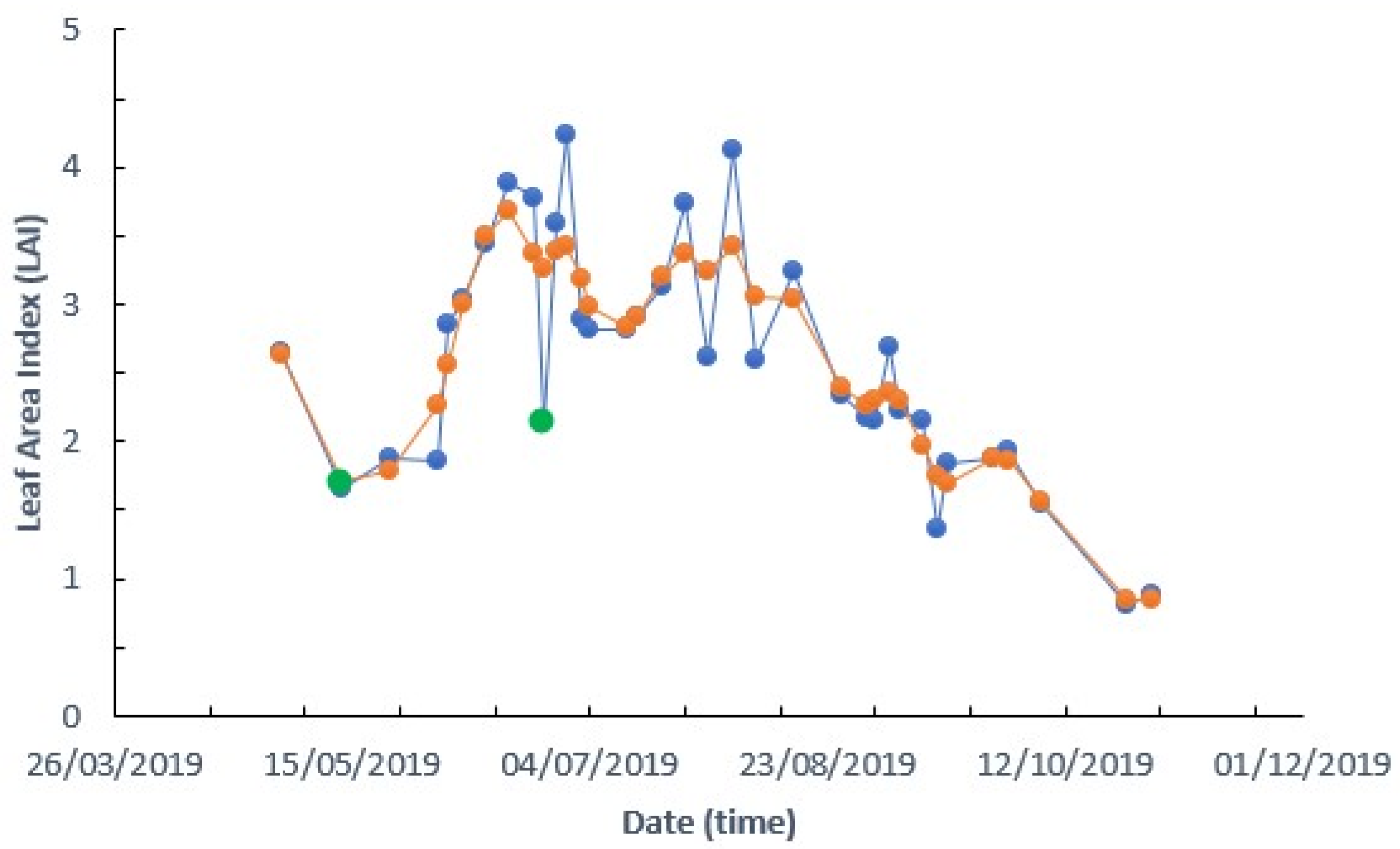
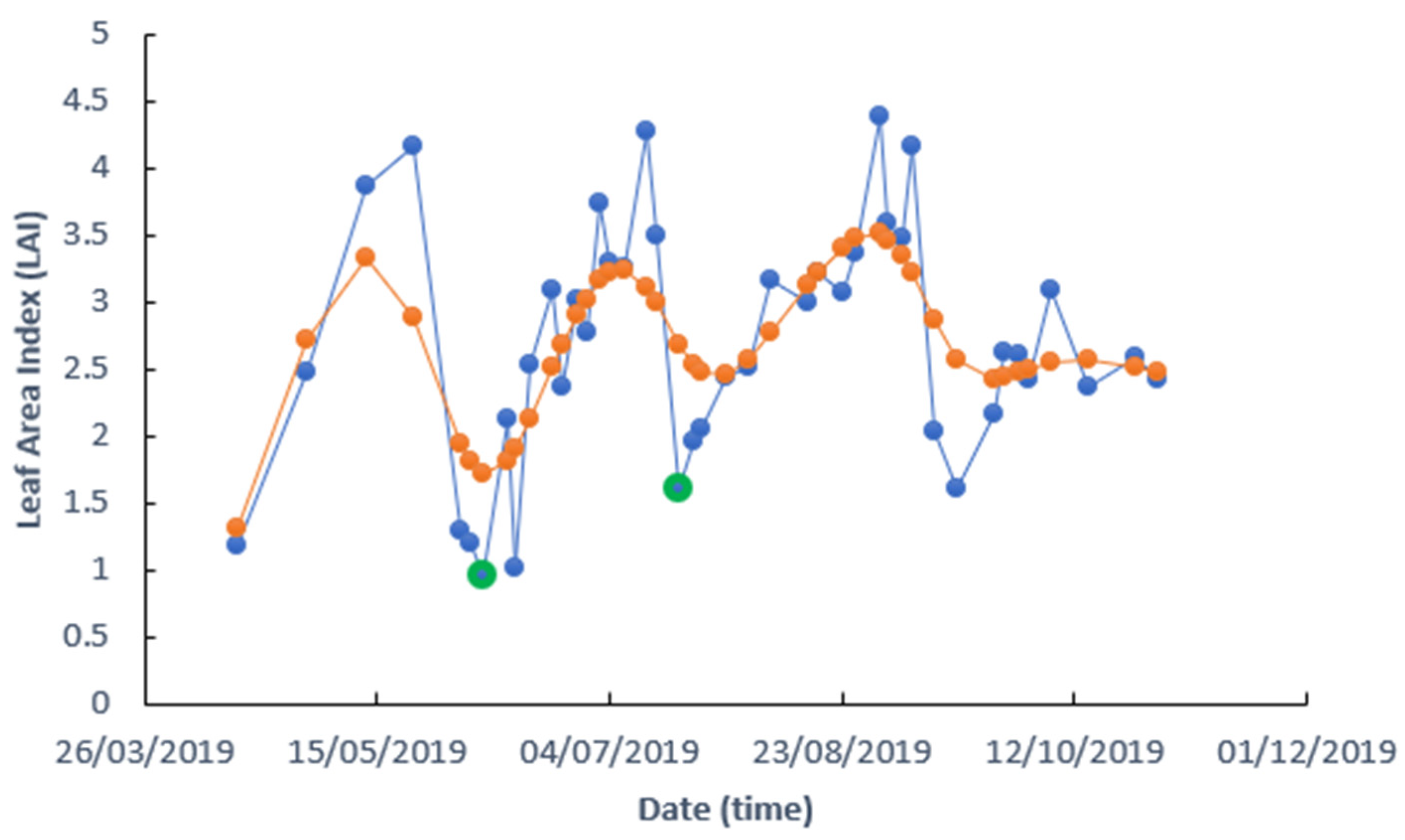
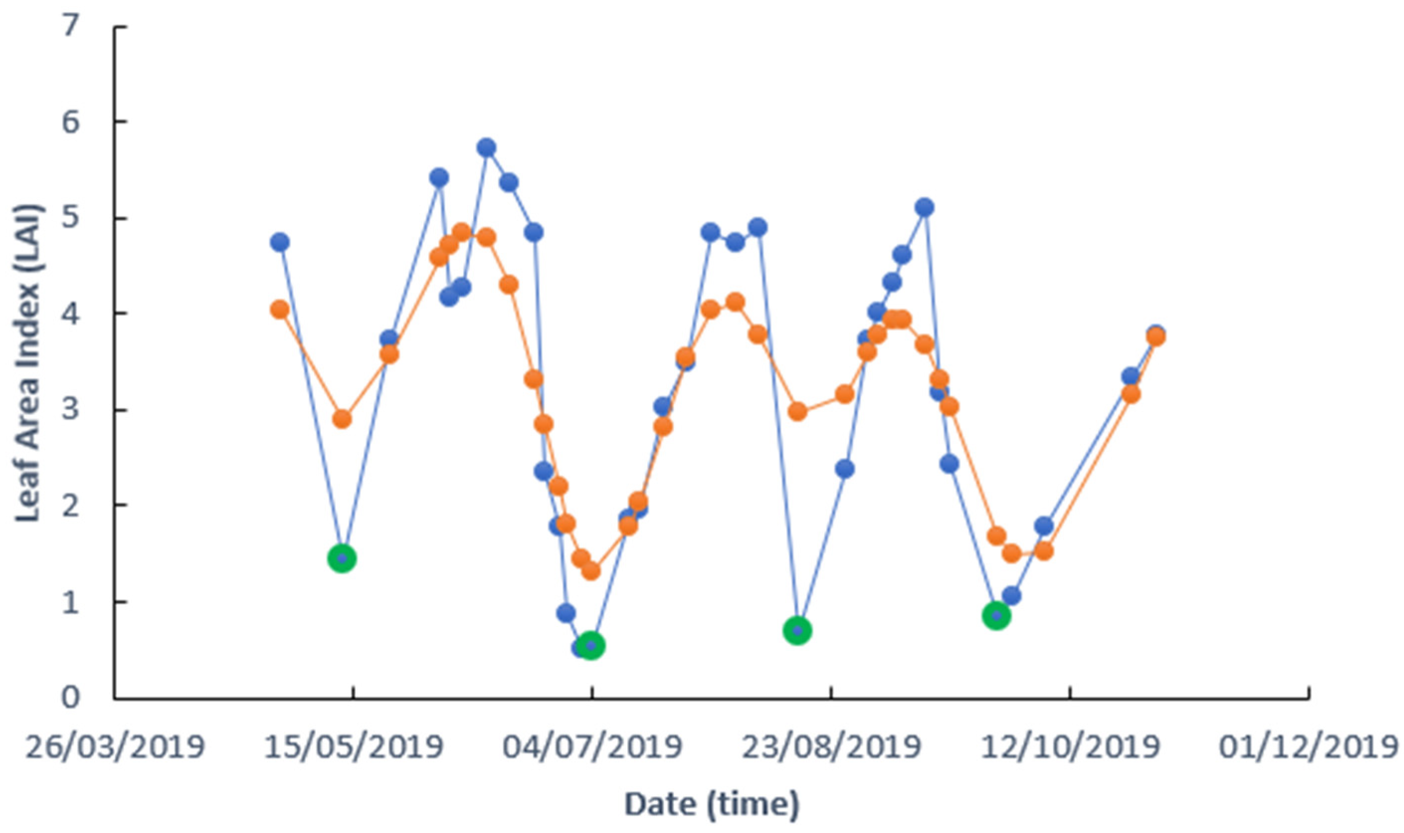
  • There are at least 2 mowing events during the May to October period. If most of the irrigated grassland is managed with 3 or 4 mowing events, this threshold makes it possible to consider less intensively managed grasslands or to allow for the possibility of missing a mowing event due to an unfavourable time series with a long cloudy period during the mowing period. Such a situation can happen even in the Mediterranean area despite the high revisit frequencies of Sentinel-2 satellites.
  • A mowing event is characterized by a local minimum with significant variations in LAI over 45 days before and after this minimum. The period of 45 days after the minimum reflects the growth time of the grassland after mowing. The period of 45 days before may seem long since a mowing induces an immediate drop in the amount of vegetation. However, we found that some mowings were delayed and then the grassland began to senesce, resulting in a decrease in green leaf area as captured by the LAI estimate. A shift of 10 to 20 days in the maximum LAI before mowing can thus be observed. In addition, gaps in LAI time series may lead to the maximum being sought over a somewhat longer period.
To implement these assumptions, we propose a five steps algorithm as summarized in Figure 2
Step 1: We first flagged the LAI time series by considering that the maximum LAI must be greater than tlaimin and lower than tlaimax. The tlaimin threshold reflects the fact that irrigated grassland leads to strong vegetation development while tlaimax is dedicated to eliminating surface type on which LAI computation fails, leading to unrealistic high values.
Step 2: To eliminate local minimum due to short-term LAI variations as induced by poor atmospheric corrections, different smoothing procedures were presented in [24,26,33]. In this work, we used the smooth spline algorithm in R [34], which is efficient and flexible. The algorithm involved a degree of freedom parameter (df) by controlling the smoothing process. The minimum was then detected on the smoothed LAI time series that might be slightly delayed in comparison to the date of the corresponding minimum in the observed LAI time series.
Step 3: Some remaining anomalies in the LAI time series that might impact LAI variations computation will be corrected. When the LAI is too small, i.e., lower than tlailow, or when the difference between the observed LAI and the smoothed LAI is greater than difmax, the observed LAI is substituted by the corresponding smoothed LAI value.
Step 4: Every detected minimum in step 2 is validated according to different criteria. First, the date of the observed minimum (tmin) is searched in the observed LAI time series within a time window around the minimum detected on the smoothed series. This time window ranges from dtb1 days before and dta1 days after the date of the minimum detected in step 2. The time tmin must fall within the considered period starting at dbeg and ending at dend, which in our case is 1 May and 15 October, respectively. Then, the value of the minimum was analysed. We consider that the minimum LAI must be lower than a threshold, and this threshold is adapted according to the LAI sampling date before and after the minimum date. Indeed, if LAI is sampled loosely around the minimum, the truncation effect of the time series may result in a minimum value that is larger than the true minimum, as the vegetation may have started to grow at the time of the measurement. The threshold is, therefore, set according to the following relationship:
tminlai = tminlai0 when dt < dtmin0
tminlai = tminlai1 when dt > dtmin1
t m i n l a i = t m i n l a i 0 + d t ( d t m i n 1 d t m i n 0 ) · ( t m i n l a i 1 t m i n l a i 0 )
with dt being the time interval between the first acquisition date before and after tmin. If the minimum is validated (LAI(tmin) < tminlai), the last test was performed on the LAI variations before (within the [tmin-dtb − tmin] period) and after (within the [tmin − tmin + dta] period) that must be greater than threshlai. The period before the minimum is reduced when LAI sampling is tightened. If the measurement period of the nbb observations before the minimum is shorter than dtb, then this period is used to calculate the LAI variation.
Step 5: The number of validated minimums, considered as mowing events, is established and used to apply the irrigated grassland filter being a minimum of two events.
The algorithm is applied at the pixel level. However, due to plot heterogeneity or border effects, an aggregation was performed within the plot boundary after applying a buffer of 20 m to provide a classification at the plot level. A plot was then declared as irrigated grassland when a majority of pixels were classified as irrigated grassland, the majority being qualified by a percentage of the pixels that has to be determined (pixperc).
The detection algorithm involved 16 parameters that are summarized in Table 2. As the number of parameters was large, we prescribed some of them to values consistent with our agronomical knowledge while the other parameters were calibrated.

2.4. Calibration and Evaluation

The calibration procedure targeted the best parameters used for the separation of IPG from NIG. The calibration was performed by considering 29 vignettes surrounding a known IPG plot. In each vignette, we determined 6 polygons, 3 being inside the grassland plot and three being outside (Figure 3), that correspond to surfaces that might be orchards, vineyards, field crops, market gardens, and dry grasslands. Each polygon is considered as a single entity on which metrics describing the mowing event number distribution are computed.
The cost function used for calibration was the percentage of well-classified polygons, i.e., having a majority of pixels with at least 2 mowing events for the IPG polygons and lower than 2 for the NIG polygons. A database covering the 2016–2020 period was generated, considering that each year provides a set of data to compute the cost function.
Two phases are considered in the calibration. First, based on agronomic knowledge and/or visual analysis of LAI time series, we set dta and dtb to 45 days, dta1 to 15 days, dtb1 to 25 days, and dbeg and dend set to 1 May and 15 October, respectively. Then, fd, tlaimax, tlaimin, threslai, and pixperc were calibrated using a manual fitting considering the range of value provided in Table 2. In that first calibration phase, the LAI anomaly correction (step 3) and the filtering tests on the minimum value (step 4) involving the other parameters were not activated.
Then, in a second phase, some refinements were added to the minimum detection algorithm dtlimlai0, dtlimlai1, dtmin0, dtmin1, and tlailow were prescribed to 15, 25, 10, 25, 2, 2.5, and 0.4, respectively, based on the visual analysis of the LAI time series that led to an error in the first phase. The other parameters (difmax and nbb) were calibrated.
The evaluation was made at the plot level on 780 plots not used for the calibration with 362 IPG plots and 418 NIG plots, in which their break down is 162 orchards; 100 vineyards; 99 greenhouses; 20 dry grass; 33 field crops; and 4 lawns.

2.5. Accuracy Assessment

Accuracy assessment remains an important aspect of mapping projects utilising remotely sensed information [35]. The different classifications made in the study were evaluated using overall accuracy (OA), producer’s accuracy (PA), and Cohen’s Kappa index (K), all quantities being derived from the confusion matrix having the following terms: TG (well-classified irrigated grassland plots), FG (plot classified as irrigated grassland while not an irrigated grassland), TNG (well classified not irrigated grassland plots), and FNG (irrigated grassland plot classified as not irrigated grassland).
O v e r a l l   a c c u r a c y =   T G + T N G   T G + F G + T N G + F N G · 100
Producer’s accuracy corresponds to the error due to omission (exclusion). From the perspective of the land use map maker, it indicates how accurate is the map: For a given class, it shows how many plots among the reference plots in the map were tagged accurately. It is defined for = IPG as follows.
P r o d u c e r s   a c c u r a c y = T G   T G + F N G · 100  
Cohen’s Kappa index (K) characterizes the map agreement with the ground truth after removing the chance factor. It is an indication of the adding value of the classification method, which is defined as follows:
K = o v e r a l l   a c c u r a c y     c h a n c e   a g r e e m e n t 1 c h a n c e   a g r e e m e n t
where chance agreement is the probability of having a good classification by chance, which is defined by the following.
c h a n c e   a g r e e m e n t = ( T G + F G ) · ( T G + F N G ) + ( F N G + T N G ) · ( F G + T N G ) ( T G + F G + F N G + T N G ) 2

2.6. Benchmark

Different existing classification methods based on Sentinel 2 data were considered to assess the adding value of the new proposed method described above. First, we made a supervised classification based on the Support Vector Machine (SVM) method, which is rather common and powerful for discriminating two classes. The classification was carried out on cloud-free LAI images taken over the entire year. Due to the proximity of the coast, we have large cloudiness heterogeneities. To maximise the number of images, the Crau area was divided into four zones, and for each zone, we selected the images according to the following two criteria: (1) The entire zone is cloud free as well as (2) for the training polygons (Figure 3). As a consequence, the number of images used for the classification varied between 12 and 25 in 2016, 13 and 33 in 2017, and 24 and 38 in 2018 according to the zones. The training dataset is similar to that used for the developed algorithm by taking randomly three pixels in every polygon described in Section 2.5. The training was performed for each year with the cloud-free images selected for each of the four zones. The classification was then applied to each zone and aggregated over the Crau area to produce a binary image (IPG/NIG) per year.
We also consider the THEIA land use map as a benchmark since it is implemented yearly over the entire national territory (https://www.theia-land.fr/ceslist/ces-occupation-des-sols/, accessed on 17 May 2022). It is a supervised classification [36] based on random forest classification using all Sentinel-2 dates and the VIS and NIR bands and as auxiliary information, including the topography, urban map, Corinne Land Cover map, and the RPG (‘Registre Parcellaire Graphique) data, which gather farmer’s annual declarations for obtaining subsidies from the European Union. Seventeen classes were identified with one dedicated to grasslands. In our study, the detection of one class, the grassland class, among the others was evaluated. The produced maps are provided at the scale of Sentinel 2 10 m pixels.
The evaluation of the two benchmark classifications was performed on the evaluation plots described in Section 2.5. Therefore, each evaluation plot is classified according to the majority class (>50% of the pixels in the plot).

3. Results

3.1. Calibration

The most important parameter is the smoothing parameter (df) for which its effect is clearly illustrated in Figure 4, Figure 5 and Figure 6. The goal of the smoothing is to remove signal oscillations that are not linked to mowing events (Figure 4). We observed that most of these undesirable oscillations correspond to short-term variations. Therefore, the smoothing should be strong enough to remove them (i.e., df < 15) but should not be too strong as some mowing events might be missed (i.e., df = 5). The calibration led to df = 10, which corresponds to an intermediate case in Figure 5. When applying the minimum detection on the smoothed LAI time series, we identified three events that are consistent with the mowing calendar (Figure 6). The rate of misclassified plots was about 13% after phase 1 (Table 3). The main source of error comes from the detection of NIG as IPG (9%), as shown in Figure 7.
In the presented case in Figure 7, smoothing was not appropriate and some strong LAI oscillations were still present in the smoothed signal, thus triggering the identification of false mowing events. However, the LAI values corresponding to the detected minimum were high and larger than what is expected with freshly mowed grass. An additional test on the LAI values at the detected minimum is a way to resolve the ambiguity displayed in Figure 7. The analysis of such errors led to defining the series of tests and data manipulation, as described in Section 2.3 in steps 3 and 4, and the parameters were characterized in phase 2. After this phase, we reduced the misclassified plots rate to less than 4%, with still a greater probability to miss an NIG than an IPG (Table 3). The final values of the parameters of the algorithm are reported in Table 2.
To illustrate the results of the algorithm, we selected an area covering two grassland plots surrounded by NIG area. The results obtained in 2019 are displayed in Figure 8 where letters represent the exact location of the pixel time series A, B, and C displayed in Figure 6, Figure 9 and Figure 10, respectively. There is a clear difference in grass management with four mowing events in the northern plot and three in the southern (Figure 8), as illustrated in Figure 6 and Figure 10. If the plots are mostly homogeneous, some areas with less mowing events can be seen at the plot boarder, in the middle corresponding to a ditch bringing the water, and in some patches. The case of point A (Figure 9) indicates that the missed last mowing event is explained by a low grass growth at end of the season. The difference between the minimum and the maximum after harvest was below 1.5 (threshlai < 1.5), reflecting less productive area that might be induced by soil properties or the quality of the irrigation with heterogeneities induced by poor soil levelling.

3.2. Evaluation

Results obtained on the evaluation data set are provided in Table 4. Excellent results were obtained with an OA greater than 97% and a Kappa index between 0.94 and 0.99. The producer accuracy is equal to 100% for the NIG class, meaning that a parcel declared as a NIG is always NIG. This shows that additional filtering can handle situations such as the one shown in Figure 7. The producer’s accuracies of the IPG class are a little less good, which means that some IPG plots are not detected. We will come back to this point in the Discussion section. There is also a year effect that appears clearly. For example, 2020 was the worst year, while the best results were obtained in 2018. The 2018 year is the wettest year during the summer, which might limit the irrigation pressure and, therefore, allowed good production throughout the cycle. In 2020, there was gap of 20 days in the measurements, which did not allow for the detection of the maximum grass development between the second and the third mowing events, leading to missing both of them.
These good results have to be tempered by the fact that IPGs are likely a class that is easy to detect, as shown by the good results depicted in Table 4 with THEIA classification approaches. However, our results are clearly better than those obtained with the SVM method, which means that algorithms based on artificial intelligence cannot necessarily capture the agronomic traits as used in our method. Although slightly better, our results are comparable to those of THEIA, which relies on a rich spatialized ground truth with the administrative census and Corinne Land Cover data.

4. Discussion

The proposed method was applied to the entire territory of the Crau area having 18,058 plots with an illustration given in Figure 11 for the year 2018, showing all plots of IPG (in green) and NIG (in red). We do not have any reference on the entire territory; we can, therefore, only make relative analyses. This was performed by addressing the following two questions: (i) What is the impact of classifying land use at plot scale compared to a pixel scale approach? (ii) What is the evolution of irrigated areas between years and can it be linked to changes in land use? Finally, we discussed the novelty of the approach and its generalisation

4.1. Impact of Plot Aggregation in the Classification Process

One of the constraints of the method applied in this work is that the land-use class is determined at the scale of a plot. We have seen in Figure 8 that the edges of the plot, the irrigation ditches within the plot, and certain less productive areas could lead to a lower number of mows and thus induce a misclassification of the pixel. It is also possible to have isolated pixels located in NIG areas that present several mowing-like events. Working at the plot level reduces the risk of error since the land-use class is based on a majority of pixels. However, a plot map with their boundaries is not always available, especially when large areas are considered. Furthermore, the plot map may contain errors generating errors in the areas counted or misclassification of an IPG plot when it includes a significant part (>10% in our case) of an area that is not an IPG. For inventory purposes, we can imagine applying the developed classification method at the pixel level rather than at the plot level. To see the impact of such a choice, we compared the total surface over the Crau area obtained using either a pixel-based approach by counting the pixels classified in each class or a plot-based approach where we summed the surface of the plots per class.
The pixels of the study site (the Crau) were taken from an extraction polygon that is as close as possible to the considered area being the aggregation of plots. As this area sometimes presents a complex boundary (Figure 11), the extracted polygon was drawn inside the area explaining the small differences in the total areas of the pixel based and plot base counting (Table 5). The percentages of IPG based on the plot-based approach ranged from 25 to 26% and 74 to 75% for NIG, while for the pixel-based approach, the percentages of IPG ranged from 22 to 25% and 75 to 78% for NIG. The underestimation obtained with the pixel-based approach, likely due to plot boarder effect, remained, however, moderate.

4.2. Ability to Detect Land-Use Changes

The proposed method implemented across the five years (2016–2020) provided us with an overview of the consistency of the results from one year to another. Results are displayed in Table 6 by considering plots where the classification remained stable over the five years (i.e., GGGGG and NNNNN classes), plots that met one change that can be attributed to a land-use change, and plot having several changes, reflecting problems in their classification. In 91% of the case, perfect stability was observed. The analysis was conducted on plots presenting one change with spatial illustrations depicted in Figure 12. The figure shows that changes are spread over the area with plot of different sizes. The causes of the change were identified by analysing the high-resolution images acquired during the considered period. From these images, we can identify the following key features clearly:
LUC: land-use change, most of them being IPG converted in urban areas, orchards or abandon and vice versa;
EXPL: Some plots have been levelled and resown, and the algorithm can fail to classify such plots as IPG, especially during the first year after leveling because there is relatively very low vegetation growth;
MGT: Some plots are very heterogeneous likely due to permanent grazing or irrigation problems such as the insufficient flow of irrigation water or a lack of levelling preventing a homogeneous water supply;
In the other cases, hereafter labelled as ERR, there were no clear features that can explain the classification change during the considered period.
Analysis of the data in Table 6 shows that over the 5 years, 607 (6%) plots presented one change in classification while 331 (3%) plots had at least two changes. The analysis of the high-resolution images on plots with time series presenting at least one change shows that when a plot is detected as an IPG, it is always an IPG. On the 707 plots controlled, only one case corresponding to a young grassed orchard generated an error. This confirms the reliability of the algorithm when IPG is detected, as shown in Table 4, with a producer accuracy close to 100%. Among plots with at least one year classified as IPG (class Id 1, 3–11 in Table 6), 19% have discontinuous NIG-IPG series over the 5 years. These plots are mostly related to heterogeneity problems (MGT) (66% of the cases), while in 27% of the cases, a real change in use (LUC) or a plot levelling (EXPL) was observed. If we consider the cases where the change is confirmed over the last 2 or 3 years (Case ID 4, 5, 8, 9), the cumulative rate of LUC and EXPL features increased to 50%.
This leads us to conclude that the use of a long series (5 years) allows us to characterise IPGs even when they present strong heterogeneities linked to irrigation defects or grazing during the summer period. The occurrence of IPG detection could be a marker of grassland management and might be used as information to refine the description of grassland systems. The detection of real land-use change needs confirmation of the change over several years (>3 years), which requires a time series longer than 5 years to reduce the ambiguity between actual land use change and classification errors induced by grassland management.

4.3. Novel Aspects and Generalization

Our study shows that a classification based on temporal signal with agronomic trait detection offers much better results than a supervised classification such as the use of the SVM method. This superiority is probably exacerbated with the detection of intensively farmed grasslands. Indeed, with grasslands, there is no strong seasonality in vegetation variation. Vegetation cycles are numerous and asynchronous between IPG plots, making the identification of a specific grassland pattern in the data series across the entire Crau area difficult by a simple supervised classification algorithm such as SVM. This comparison is somewhat contradicted by the very good results obtained by THEIA, which also used a supervised random forest classification. However, the a priori knowledge on the territory integrated in the classification can have a very important weight in the obtained performances, and it would be interesting to analyse the impact of remotely sensed classifiers on the results. If classification approaches based on agronomic traits detection are efficient, they remain specific to a given class of land use and are not adapted for simultaneously identifying a large number of classes as could be performed by usual classification methods. Thus, a complementarity between methods might be foreseen, where approaches based on the temporal signal should be dedicated to answering some specific questions requiring a good accuracy on a given land use class as for IPG in the Crau area.
The advantage of our method is that it does not require supervised learning even if some calibration was required on a few plots. The question is then to establish to what extent our approach is generic and implementable in other contexts. First, we found that a single set of parameters was suitable for the five years. The analysis of the classification errors has shown that classification errors come more from ground problems (plot heterogeneity and management variability) and the timing of the LAI time series than the detection algorithms itself. Thus, we can reasonably support the idea that calibrated algorithms can be applied to any years. The implementation of the development method to other territories needs to be examined more carefully. Most of the parameters (10 over 16) were prescribed either from agronomic knowledge (dta1, dtb1, dta, dtb, tminlai0, tminlai1, dtmin0, dtmin1, and tlailow) or on visual analysis on some problematic LAI time series (difmax). We think that these parameters can be adapted to other contexts. As far as the calibrated parameters are concerned, they have to be considered individually. Nbb and fd are related to the temporal frequency of the images. It is conceivable that, in a cloudier context, they may have to be revisited. threshlai and tlaimin are related to the temporal dynamics of the LAI of grasslands, which is influenced by plot management and soil and climate conditions. However, with a good knowledge of the grasslands of the targeted territory, it should be possible to provide an estimation for both parameters. This was the case in our study with tlaimin for which its values were explored over a narrow range (from 4.0 to 4.5). The filtering of outliers with tlaimax seems to us to have a generic scope while the pixperc parameter could be the most impacted by new contexts with different intra-plot heterogeneities. In conclusion, we think that adaptations of the parameters based on the knowledge of the territorial characteristics of the grasslands should allow good accuracy. A calibration will undoubtedly be necessary to obtain the precision levels obtained in our study, but this must be performed only once for all years.
Several algorithms, comparable to the one above, have recently been published [23,24,26,27]. While the approaches used are similar, the solutions for filtering the signal from atmospheric remaining effects and detecting drops in the time series of vegetation indices are very different. It is, however, difficult to compare our results with those of these studies since we are interested in the identification of grasslands whereas the other studies are interested in the number of mowing events that is sought. In all cases, the timing of the time series and the diversity of the grasslands due to their management or heterogeneity lead to detection errors. In spite of the good scores obtained in our classifications, we had mowing detection errors that did not necessarily lead to a classification error, since the observation of two events is sufficient to classify IPTs even though they are mowed three or four times a year. We can also point out that the complexity of the mowing detection algorithms is largely due to anomalies in the temporal series of the vegetation index. This could be simplified if the data were better filtered upstream, and there is no doubt that this will be possible in the future. In this sense, the approach in [27] to improve cloud masks is interesting.

5. Conclusions

A new algorithm for the identification of Irrigated Permanent Grass (IPG) was developed in this study. It is based on the detection of agronomic traits thanks to the possibility offered by the Sentinel 2 mission to provide frequent images of the vegetation development. In our area located in the Mediterranean, about 40 images per year can be exploited during the period of interest (mid-April to October ending). IPGs were classified by detecting mowing events assuming that a pixel is an IPG when at least two mowing events were detected. The developed classification method offers very good results, better than that obtained when using supervised classification as SVM or land use product as the THEIA product covering the French territory. The method presents the advantage of not depending on training samples, even if some calibration was necessary to fix some thresholds and deal with the remote sensing signal noise. We believe that calibration efforts will likely be lower when addressing IPG detection in other geographical contexts. Moreover, once established, the algorithm can be applied directly to another year.
Despite the good performance of the developed algorithm, it is faced with some constraints that lead to failure to detect mowing activities. For instance, when there is relatively very low biomass or a heterogeneous plot, the developed algorithm tends to fail by missing some mowing events. This can be seen as a weakness, but our analysis has shown that the IPG class covers several management modalities. Depending on the objectives, such a weakness can be a strength to characterize different production systems. In addition, the detection of mowing should make it possible to understand the technical itineraries and to provide information to inform farming practice heterogeneities over large territory to implement crop models. Real changes in use can be observed, but long time series are needed to confirm the change and remove ambiguities with heterogeneous grasslands.
In general, one can question the relevance of relying on agronomic traits specific to certain types of land use to map them. In this work, we have relied on a clear, specific, and somewhat caricatural trait, and this has obtained excellent results. The results in the literature are not necessarily as precise, and this is probably due to less clear specific features that can lead to ambiguities. We believe, for example, that the separation of vineyards and orchards, which is important to map different irrigation strategies, may be more difficult to characterize. Moreover, it was found that the method requires frequent acquisition to catch the events of interests. For locations with frequent cloud cover, combining optic and radar images can be an option to overcome the lack of optical data.

Author Contributions

Conceptualization, M.A. and A.C.; Data curation, M.A., G.P. and F.F.; Formal analysis, M.A.; Methodology, M.A., A.C. and G.P.; Software, G.P.; Supervision, A.C. and D.C.; Writing—original draft, M.A. and A.C.; Writing—review & editing, M.A., A.C. and D.C. All authors have read and agreed to the published version of the manuscript.

Funding

This work was funded by Petroleum Technology Development Fund (PTDF) under the Federal Ministry of Petroleum, Nigeria, in collaboration with INRAE-EMMAH Avignon as part of a PhD research program.

Data Availability Statement

Sentinel 2 data are available at the following hyperlink: https://www.theia-land.fr/, accessed on 17 May 2022. THEIA classification data can be found at the following hyperlink: https://www.theia-land.fr/ceslist/ces-occupation-des-sols/, accessed on 17 May 2022. Inglada, Jordi, Vincent, Arthur, & Thierion, Vincent. (2018). Theia OSO Land Cover Map 2018 [Data set]. Zenodo. https://doi.org/10.5281/zenodo.3613415 (accessed on 17 May 2022). plot boundary map and evaluation data over the CRAU are available on request from the corresponding author. The data are not publicly available due to personal data in the data set.

Acknowledgments

The authors would like to thank the reviewers for helping us improve the quality of this research work.

Conflicts of Interest

The authors declare no conflict of interest.

References

  1. International Decade for Action on Water for Sustainable Developmen. 2016. Available online: https://www.un.org/en/events/waterdecade/background.shtml (accessed on 14 April 2022).
  2. Wriedt, G.; Van der Velde, M.; Aloe, A.; Bouraoui, F. Estimating Irrigation Water Requirements in Europe. J. Hydrol. 2009, 373, 527–544. [Google Scholar] [CrossRef]
  3. Wada, Y.; Wisser, D.; Eisner, S.; Flörke, M.; Gerten, D.; Haddeland, I.; Hanasaki, N.; Masaki, Y.; Portmann, F.T.; Stacke, T.; et al. Multimodel Projections and Uncertainties of Irrigation Water Demand under Climate Change. Geophys. Res. Lett. 2013, 40, 4626–4632. [Google Scholar] [CrossRef] [Green Version]
  4. Marras, P.A.; Lima, D.C.A.; Soares, P.M.M.; Cardoso, R.M.; Medas, D.; Dore, E.; De Giudici, G. Future Precipitation in a Mediterranean Island and Streamflow Changes for a Small Basin Using EURO-CORDEX Regional Climate Simulations and the SWAT Model. J. Hydrol. 2021, 603, 127025. [Google Scholar] [CrossRef]
  5. Bazzi, H.; Baghdadi, N.; Ienco, D.; El Hajj, M.; Zribi, M.; Belhouchette, H.; Jose Escorihuela, M.; Demarez, V. Mapping Irrigated Areas Using Sentinel-1 Time Series in Catalonia, Spain. Remote Sens. 2019, 11, 1836. [Google Scholar] [CrossRef] [Green Version]
  6. Gao, Q.; Zribi, M.; Escorihuela, M.; Baghdadi, N.; Segui, P. Irrigation Mapping Using Sentinel-1 Time Series at Field Scale. Remote Sens. 2018, 10, 1495. [Google Scholar] [CrossRef] [Green Version]
  7. Ambika, A.K.; Wardlow, B.; Mishra, V. Remotely Sensed High Resolution Irrigated Area Mapping in India for 2000 to 2015. Sci. Data 2016, 3, 160118. [Google Scholar] [CrossRef] [PubMed] [Green Version]
  8. Massari, C.; Modanesi, S.; Dari, J.; Gruber, A.; De Lannoy, G.J.M.; Girotto, M.; Quintana-Segui, P.; Le Page, M.; Jarlan, L.; Zribi, M.; et al. A Review of Irrigation Information Retrievals from Space and Their Utility for Users. Remote Sens. 2021, 13, 4112. [Google Scholar] [CrossRef]
  9. Ozdogan, M.; Gutman, G. A New Methodology to Map Irrigated Areas Using Multi-Temporal MODIS and Ancillary Data: An Application Example in the Continental US. Remote Sens. Environ. 2008, 112, 3520–3537. [Google Scholar] [CrossRef] [Green Version]
  10. Deines, J.M.; Kendall, A.D.; Hyndman, D.W. Annual Irrigation Dynamics in the US Northern High Plains Derived from Landsat Satellite Data. Geophys. Res. Lett. 2017, 44, 9350–9360. [Google Scholar] [CrossRef]
  11. Maselli, F.; Battista, P.; Chiesi, M.; Rapi, B.; Angeli, L.; Fibbi, L.; Magno, R.; Gozzini, B. Use of Sentinel-2 MSI Data to Monitor Crop Irrigation in Mediterranean Areas. Int. J. Appl. Earth Obs. Geoinf. 2020, 93, 102216. [Google Scholar] [CrossRef]
  12. Pun, M.; Mutiibwa, D.; Li, R. Land Use Classification: A Surface Energy Balance and Vegetation Index Application to Map and Monitor Irrigated Lands. Remote Sens. 2017, 9, 1256. [Google Scholar] [CrossRef] [Green Version]
  13. Demarez, V.; Helen, F.; Marais-Sicre, C.; Baup, F. In-Season Mapping of Irrigated Crops Using Landsat 8 and Sentinel-1 Time Series. Remote Sens. 2019, 11, 118. [Google Scholar] [CrossRef] [Green Version]
  14. Pageot, Y.; Baup, F.; Inglada, J.; Baghdadi, N.; Demarez, V. Detection of Irrigated and Rainfed Crops in Temperate Areas Using Sentinel-1 and Sentinel-2 Time Series. Remote Sens. 2020, 12, 3044. [Google Scholar] [CrossRef]
  15. Julien, Y.; Sobrino, J.A.; Jiménez-Muñoz, J.-C. Land Use Classification from Multitemporal Landsat Imagery Using the Yearly Land Cover Dynamics (YLCD) Method. Int. J. Appl. Earth Obs. Geoinf. 2011, 13, 711–720. [Google Scholar] [CrossRef]
  16. Karantzalos, K.; Karmas, A.; Tzotsos, A. Monitoring Crop Growth and Key Agronomic Parameters through Multitemporal Observations and Time Series Analysis from Remote Sensing Big Data. Adv. Anim. Biosci. 2017, 8, 394–399. [Google Scholar] [CrossRef]
  17. Ashourloo, D.; Shahrabi, H.S.; Azadbakht, M.; Aghighi, H.; Nematollahi, H.; Alimohammadi, A.; Matkan, A.A. Automatic Canola Mapping Using Time Series of Sentinel 2 Images. ISPRS J. Photogramm. Remote Sens. 2019, 156, 63–76. [Google Scholar] [CrossRef]
  18. Ashourloo, D.; Shahrabi, H.S.; Azadbakht, M.; Rad, A.M.; Aghighi, H.; Radiom, S. A Novel Method for Automatic Potato Mapping Using Time Series of Sentinel-2 Images. Comput. Electron. Agric. 2020, 175, 105583. [Google Scholar] [CrossRef]
  19. Merot, A.; Bergez, J.-E.; Capillon, A.; Wery, J. Analysing Farming Practices to Develop a Numerical, Operational Model of Farmers’ Decision-Making Processes: An Irrigated Hay Cropping System in France. Agric. Syst. 2008, 98, 108–118. [Google Scholar] [CrossRef]
  20. Dusseux, P.; Vertes, F.; Corpetti, T.; Corgne, S.; Hubert-Moy, L. Agricultural Practices in Grasslands Detected by Spatial Remote Sensing. Environ. Monit. Assess. 2014, 186, 8249–8265. [Google Scholar] [CrossRef]
  21. Gómez Giménez, M.; de Jong, R.; Della Peruta, R.; Keller, A.; Schaepman, M.E. Determination of Grassland Use Intensity Based on Multi-Temporal Remote Sensing Data and Ecological Indicators. Remote Sens. Environ. 2017, 198, 126–139. [Google Scholar] [CrossRef]
  22. Stumpf, F.; Schneider, M.K.; Keller, A.; Mayr, A.; Rentschler, T.; Meuli, R.G.; Schaepman, M.; Liebisch, F. Spatial Monitoring of Grassland Management Using Multi-Temporal Satellite Imagery. Ecol. Indic. 2020, 113, 106201. [Google Scholar] [CrossRef]
  23. Courault, D.; Hadria, R.; Ruget, F.; Olioso, A.; Duchemin, B.; Hagolle, O.; Dedieu, G. Combined Use of FORMOSAT-2 Images with a Crop Model for Biomass and Water Monitoring of Permanent Grassland in Mediterranean Region. Hydrol. Earth Syst. Sci. 2010, 14, 1731–1744. [Google Scholar] [CrossRef] [Green Version]
  24. Schwieder, M.; Wesemeyer, M.; Frantz, D.; Pfoch, K.; Erasmi, S.; Pickert, J.; Nendel, C.; Hostert, P. Mapping Grassland Mowing Events across Germany Based on Combined Sentinel-2 and Landsat 8 Time Series. Remote Sens. Environ. 2022, 269, 112795. [Google Scholar] [CrossRef]
  25. Lobert, F.; Holtgrave, A.-K.; Schwieder, M.; Pause, M.; Vogt, J.; Gocht, A.; Erasmi, S. Mowing Event Detection in Permanent Grasslands: Systematic Evaluation of Input Features from Sentinel-1, Sentinel-2, and Landsat 8 Time Series. Remote Sens. Environ. 2021, 267, 112751. [Google Scholar] [CrossRef]
  26. Andreatta, D.; Gianelle, D.; Scotton, M.; Vescovo, L.; Dalponte, M. Detection of Grassland Mowing Frequency Using Time Series of Vegetation Indices from Sentinel-2 Imagery. GIScience Remote Sens. 2022, 59, 481–500. [Google Scholar] [CrossRef]
  27. Kolecka, N.; Ginzler, C.; Pazur, R.; Price, B.; Verburg, P.H. Regional Scale Mapping of Grassland Mowing Frequency with Sentinel-2 Time Series. Remote Sens. 2018, 10, 1221. [Google Scholar] [CrossRef] [Green Version]
  28. Taravat, A.; Wagner, M.; Oppelt, N. Automatic Grassland Cutting Status Detection in the Context of Spatiotemporal Sentinel-1 Imagery Analysis and Artificial Neural Networks. Remote Sens. 2019, 11, 711. [Google Scholar] [CrossRef] [Green Version]
  29. De Vroey, M.; Radoux, J.; Defourny, P. Grassland Mowing Detection Using Sentinel-1 Time Series: Potential and Limitations. Remote Sens. 2021, 13, 348. [Google Scholar] [CrossRef]
  30. Séraphin, P.; Vallet-Coulomb, C.; Gonçalvès, J. Partitioning Groundwater Recharge between Rainfall Infiltration and Irrigation Return Flow Using Stable Isotopes: The Crau Aquifer. J. Hydrol. 2016, 542, 241–253. [Google Scholar] [CrossRef]
  31. Trolard, F.; Bourrié, G.; Baillieux, A.; Buis, S.; Chanzy, A.; Clastre, P.; Closet, J.-F.; Courault, D.; Dangeard, M.-L.; Di Virgilio, N.; et al. The PRECOS Framework: Measuring the Impacts of the Global Changes on Soils, Water, Agriculture on Territories to Better Anticipate the Future. J. Environ. Manag. 2016, 181, 590–601. [Google Scholar] [CrossRef]
  32. Weiss, M.; Baret, F.; Leroy, M.; Hautecoeur, O.; Bacour, C.; Prevot, L.; Bruguier, N. Validation of Neural Net Techniques to Estimate Canopy Biophysical Variables from Remote Sensing Data. Agronomie 2002, 22, 547–553. [Google Scholar] [CrossRef] [Green Version]
  33. Tian, J.; Zhu, X.; Chen, J.; Wang, C.; Shen, M.; Yang, W.; Tan, X.; Xu, S.; Li, Z. Improving the Accuracy of Spring Phenology Detection by Optimally Smoothing Satellite Vegetation Index Time Series Based on Local Cloud Frequency. ISPRS J. Photogramm. Remote Sens. 2021, 180, 29–44. [Google Scholar] [CrossRef]
  34. Hastie, T.J.; Tibshirani, R.J. Generalized Additive Model; Chapman and Hall/CRC: London, UK, 1990; ISBN 978-0-412-34390-2. [Google Scholar]
  35. Congalton, R.G. Accuracy Assessment and Validation of Remotely Sensed and Other Spatial Information. Int. J. Wildland Fire 2001, 10, 321–328. [Google Scholar] [CrossRef] [Green Version]
  36. Inglada, J.; Vincent, A.; Arias, M.; Tardy, B.; Morin, D.; Rodes, I. Operational High Resolution Land Cover Map Production at the Country Scale Using Satellite Image Time Series. Remote Sens. 2017, 9, 95. [Google Scholar] [CrossRef] [Green Version]
Figure 1. Study site location.
Remotesensing 14 03056 g001
Figure 2. Five steps of the developed irrigated grassland algorithm at the pixel level.
Remotesensing 14 03056 g002
Figure 3. Green polygons symbolise IPG while red polygons symbolise NIG.
Remotesensing 14 03056 g003
Figure 4. Observed LAI time series of an IPG pixel before smoothing; red dots correspond to LAI minimums that are not linked to mowing events. Green dots are LAI minimum linked to the mowing event.
Remotesensing 14 03056 g004
Figure 5. Effect of degrees of freedom (df) of the smoothed algorithms on LAI times series of an IPG pixel. In blue is the observed LAI; the smooth LAI times series with df equalling 5, 10 and 15 are in grey, orange, and yellow, respectively.
Remotesensing 14 03056 g005
Figure 6. Observed LAI time series (blue) and smoothed LAI time series (orange) of an IPG pixel. Green dots correspond to minimum LAI detected on the smoothed LAI time series.
Remotesensing 14 03056 g006
Figure 7. Observed (blue) and smoothed (orange) LAI time series of a NIG pixel detected as an IPG. The green dots correspond to the detected mowing events using the developed algorithm after the first phase of calibration.
Remotesensing 14 03056 g007
Figure 8. Results obtained after the second phase of calibration in 2019 showing locations of Figure 6, Figure 9 and Figure 10.
Remotesensing 14 03056 g008
Figure 9. Observed signal (blue) and smoothed (orange) LAI time series of an IPG pixel showing two mowing events (green dots).
Remotesensing 14 03056 g009
Figure 10. Observed (blue) and smoothed (orange) LAI time series of an IPG pixel showing four mowing events (green dots).
Remotesensing 14 03056 g010
Figure 11. Land use map using the developed algorithm in 2018.
Remotesensing 14 03056 g011
Figure 12. Landuse change map 2016–2020 showing changes from IPG to NIG (green) and NIG to IPG (blue) with a zoomed part.
Remotesensing 14 03056 g012
Table 1. Statistics on the number of days available over the period from 15 April to 30 October after removing the dates impacted by clouds. Filtering is carried out at the pixel level and the statistics have been calculated on all pixels of the Crau area.
YearAverageMaximumMinimum
2016263120
2017434937
2018526144
2019545948
2020495642
Table 2. List of parameters and value retained to implement the developed method.
ParametersDefinitionsRange of Values Used When CalibratedFinal Value
fdDegree of freedom of the smoothing algorithm5, 10, 15, 1710
tlaimaxLAI threshold. a pixel is declared being not a grassland when the maximum of LAI time series is greater than tlaimax10, 10.5, 11, 11.510.5
tlaiminLAI threshold. A pixel is declared not being a grassland when the maximum of the LAI time series is lower than tlaimin4.0, 4.1, 4.2, 4.3, 4.4, 4.54.2
threshlaiLAI variation threshold before and after the detected minimum 0.5, 1.0, 1.5, 2.0, 2.51.5
dta1Period to search for the true minimum after the smoothed minimum 15
dtb1Period to search for the true minimum before the smoothed minimum 25
tlailowLAI threshold to characterize unrealistic low LAI value 0.4
nbbNumber of points to consider in searching the maximum before a cut2, 4, 6, 84
dtmin1Minimum time interval between observations bracketting the minimum leading to selecting the largest tminlai (tminlai1) 25
dtmin0Maximum time interval between observations bracketting the minimum leading to selecting the smallest tminlai (tminlai0) 10
tminlai1Largest LAI threshold to validate a minimum LAI (when time sampling is sparse) 2.5
tminlai0Smallest LAI threshold to validate a minimum LAI (when time sampling is frequent) 2
dtaPeriod length after a minimum to characterize LAI variation 45
dtbPeriod length before a minimum to characterize LAI variation 45
difmaxThe difference between the observed and the smoothed LAI above which the LAI is corrected. 2.6
PixpercThe minimum rate of pixels detected as irrigated grass in a plot to classify it as an irrigated grass plot50, 70, 9090
Table 3. Calibration performance after the first and second phases on the calibration data set. TG represents well-classified irrigated grassland polygons; FG, polygons classified as irrigated grassland while not an irrigated grassland; TNG, well classified not irrigated grassland polygons; FNG, irrigated grassland polygons classified as not irrigated grassland.
Calibration PhasesTotal PlotsTGTNGFGFNG
First calibration phase7483722816926
Second calibration phase748416304253
Table 4. Summary of all the classification performances conducted in the Crau area.
YearOverall AccuracyProducer’s Accuracy (IPG)Producer’s Accuracy (NIG)Kappa Indice
Developed Classification
Leaf Area Index (Sentinel-2) + proposed algorithm
201697.795.2100.00.96
201799.198.3100.00.98
201899.799.4100.00.99
201998.897.5100.00.98
202096.993.899.70.94
THEIA Classification
Satellite image + Land use data + Supervised classification
201697.295.598.70.95
201798.696.9100.00.97
201898.497.898.90.97
Classification via Support Vector Machine (SVM)
Satellite images + supervised classification using SVM method
201667.272.668.40.51
20177178.379.10.63
201873.381.376.20.58
Table 5. Total surfaces obtained for IPG and NIG classes using the developed classification algorithm obtained with a plot aggregation or a pixel-based approaches.
Plot-Based Approach
IPGNIGTotal plots
201613,318 ha40,264 ha53,581 ha
201713,717 ha39,864 ha53,581 ha
201813,839 ha39,742 ha53,581 ha
201913,994 ha39,587 ha53,581 ha
202013,850 ha39,731 ha53,581 ha
Pixel-Based Approach
IPGNIGTotal pixels
201611,480 ha40,520 ha52,000 ha
201711,770 ha40,230 ha52,000 ha
201812,345 ha39,655 ha52,000 ha
201911,561 ha40,439 ha52,000 ha
202012,758 ha39,242 ha52,000 ha
Table 6. Composition of land-use change classes. (The land-use type sequence corresponds to the five-year succession G and N corresponding to the IPG and NIG classes, respectively).
Case IDLand-Use TypeSources of VariationsNumber of Plots > 1 ha
Consistent classification through the 5 years
1G G G G G 3156
2N N N N N 6623
Plots presenting one land-use change through the 5 years
3G G G G NMGT (60); ERR (15)75
4G G G N NMGT (34); LUC (15); EXPL (10)59
5G G N N NMGT(40); LUC (40); EXPL (20)100
6G N N N NMGT (21); EXPL (6); LUC (10)37
7N G G G GMGT (139); EXPL (14); ERR (32)185
8N N G G GMGT (27); LUC (7); EXPL(11); ERR (5)50
9N N N G GMGT (20); ERR (5); LUC(6)31
10N N N N GMGT (47); LUC (20); EXPL (3)70
Plots presenting ≥ 2 land-use changes through the 5 years
11G N G N GMGT(65); EXPL (25); ERR (10)100
12All plots 331
G = grassland; N = non-grassland.
Publisher’s Note: MDPI stays neutral with regard to jurisdictional claims in published maps and institutional affiliations.

