Abstract
The principal difficulty in extracting urban surface water using remote-sensing techniques is the influence of noise from complex urban environments. Although various methods exist, there are still many sources of noise interference when extracting urban surface water, and automatic cartographic methods with long time series are especially scarce. Here, we construct an automatic urban surface water extraction method from the combination of traditional water index, urban shadow index (USI), and land surface temperature (LST) by using the Google Earth Engine cloud computing platform and Landsat imagery. The three principal findings derived from the application of the method were as follows. (i) In comparison with autumn and winter, LST in spring and summer could better distinguish water from high-reflection ground objects, shadows, and roads and roofs covered by asphalt. (ii) The overall accuracy of Automated Water Extraction Index (AWEIsh) in Zhengzhou was 77.5% and the Kappa coefficient was 0.55; with consideration of the USI and LST, the overall accuracy increased to 96.0% and the Kappa coefficient increased to 0.92. (iii) During 1990–2020, the area of urban surface water in Zhengzhou increased, with an evident trend in expansion from 11.51 km2 in 2008 to 49.28 km2 in 2020. Additionally, possible omissions attributable to using 30m-resolution imagery to extract urban water areas were also discussed. The method proposed in this study was proven effective in eliminating the influence of noise in urban areas, and it could be used as a general method for high-accuracy long-term mapping of urban surface water.
1. Introduction
Urban surface water bodies are important to human activities and social development. Mapping and monitoring of surface water bodies are also essential to the urban ecosystem and environmental management [1]. Therefore, it is of great significance to optimize and improve the methods for urban surface water mapping to facilitate the monitoring of the dynamics of urban surface water bodies [2]. Especially for cities in which the process of urbanization is accelerating, it is increasingly important to develop an appropriate approach for surface water mapping with high accuracy in urban areas.
Based on remote-sensing big data and associated analysis methods, global surface water system maps and techniques for remote-sensing mapping of urban surface water have been developed [3,4]. Although radar and optical remote-sensing data have been widely used for mapping surface water bodies [5,6,7,8,9], it is necessary to use different analysis methods to extract water information from different data sources [10]. Owing to the abundance of optical remote-sensing data sources, many algorithms have been proposed for surface water mapping based on various kinds of multispectral images [11,12,13], including decision tree [14,15,16,17], support vector machine [18,19,20,21], random forest [22,23], deep learning [24,25], and other methods [26].
Water indexes derived from the calculations between different bands of remote sensing data are the most commonly used methods for surface water mapping [27]. Many such indexes are used to enhance the differences between surface water and background features. Early studies mainly used single-band threshold methods for water extraction, which have strong operability but cannot produce ideal results because of limitations associated with complex urban ground coverage [28]. In comparison with the single-band threshold approach, the multiband spectrum relationship method represents considerable improvement and consequently, and it has been used widely [29,30,31]. The water indices- and thresholds-based water-body-mapping algorithms have experienced a process of evolution. Here, we mainly introduced several widely used water indices- and thresholds-based algorithms for open surface water mapping by referring to previous studies. The Tasseled Cap Wetness (TCW) index is derived from the tasseled cap transformation based on six bands and separates water bodies and non-water objects by setting a threshold of 0 [32]. The Normalized Difference Water Index (NDWI) uses the normalization of the bands of green and near-infrared (NIR) to distinguish water (> 0) and non-water (< 0) objects by using the threshold of 0 [33]. The Modified Normalized Difference Water Index (MNDWI), which is based on the NDWI, replaces the band of NIR in NDWI with the band of shortwave infrared (SWIR) to eliminate the influence of surface shadows [34,35]. Additionally, through normalization of the bands of NIR and SWIR, Xiao et al. [36,37] proposed the Land Surface Water Index (LSWI) which performs reasonably well in measuring the water content of soil and vegetation. Menarguez [38] proposed a new algorithm by using the combination of each of the three water indices (NDWI, MNWI, and LSWI) with the Normalized Difference Vegetation Index (NDVI) and Enhanced Vegetation Index (EVI). The detailed information about these water indices was shown in Table 1.

Table 1.
Indexes commonly used for open surface water body mapping.
Many indexes are unable to effectively eliminate the influences associated with soil and the shadows of urban buildings. Moreover, previous studies about surface water mapping only considered the noises from shadows; the noises from urban high-reflection ground objects and the asphalt-covered ground are rarely considered. In 2014, Feyisa et al. [39] proposed the Automated Water Extraction Index (AWEI) using the bands green, blue, NIR, and SWIR. In addition, the index was divided into two formats of AWEInsh and AWEIsh according to whether there were terrain shadows around the surface water bodies. AWEIsh, which is mainly used for mapping surface water in the regions where shadows have substantial impacts, can also reduce the impacts of snow, ice, and mountain shadows to ensure continuity in river extraction. Therefore, it is also suitable for urban areas where shadows from ground objects represent the main sources of noise. However, noise associated with highly reflective ground objects or dark surfaces in cities is not considered, which could lead to the identification of pseudo-water bodies in urban areas. The existing water body indexes require the optimal threshold to be set manually or automatically according to each specific situation, and how best to set the optimal threshold remains a challenge for current research [31]. Additionally, given that water bodies often have a high specific heat capacity and low temperature, it is theoretically possible that land surface temperature (LST) could be applied to effectively distinguish surface water bodies from other objects in urban areas [40]; however, the studies about mapping urban surface water using LST are still very limited.
This study aimed to develop a novel approach for automatic urban surface water mapping and demonstrate its potential in investigating the spatial and temporal changes in urban surface water bodies in big cities. To achieve this objective, we selected the urban region of Zhengzhou City (the provincial capital of Henan in China) as the study area to investigate the performance of the new method. Firstly, we combined the AWEIsh and the Urban Shadow Index (USI) to suppress shadow noise and adopted the Otsu algorithm to automatically set the threshold of the water index; secondly, we introduced LST data to eliminate other residual noise information by assuming that the temperature of urban surface water is lower than the LST of other urban objects; finally, we investigated the spatial and temporal changes in surface water areas in the urban regions of Zhengzhou City from 1990 to 2020. This study proved that the newly proposed method was also applicable to other cities and had great potential for continuous monitoring of urban surface water bodies over a large region.
2. Materials and Methods
2.1. Study Area
Zhengzhou is the capital of Henan Province in China. The urban area comprises a vast number of buildings and industrial plants of various heights, and many reservoirs, rivers, and lakes. Therefore, it can be considered a suitably typical area for conducting the optimization and improvement in the algorithms for urban surface water mapping.
The Global Urban Boundaries vector data compiled by Li et al. [41] were used to define the physical boundary of the urban area (http://data.ess.tsinghua.edu.cn, accessed on 1 August 2021). First, we selected the main urban area of Zhengzhou. Then, we constructed a 500 m buffer zone on the main urban boundary to smooth the more jagged urban boundaries, filled in holes, and removed surrounding non-adjacent urban areas (Figure 1).
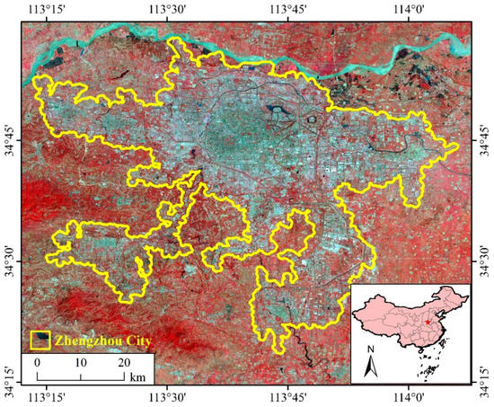
Figure 1.
Geographic location of the study area. The remote-sensing imagery in the graphic was from the data composite of Landsat 8 OLI in Zhengzhou City during June-August in 2020.
2.2. Data
2.2.1. Landsat Images
We selected images of Landsat 5 TM, 7 ETM+, and 8 OLI and used the data quality band from CFmask which is a cloud-masking algorithm to identify and remove bad-quality observations of clouds, cloud shadows, and snow [42]. Owing to certain differences in the spectral characteristics among the sensors of Landsat 5 TM, 7 ETM+, and 8 OLI [43], a linear transformation of the spectral space was applied to achieve suitable coordination in the process of synthesizing images to generate long time-series cross-sensor Landsat images. In fact, the data from the different sensors were forcibly converted and the bands were normalized.
In this study, all the available Landsat 5 TM/7 ETM+/8 OLI data including thermal infrared sensor data, top-of-atmosphere reflectance data, and surface reflectance data in the study area during April–October from 1990 to 2020 were obtained from the database of the Google Earth Engine cloud computing platform. All the steps of masking bad-quality Landsat observations were also carried out and completed on the Google Earth Engine platform. Our previous studies [44,45] have recorded the detailed steps for detecting and removing the Landsat pixels with bad-quality observations of clouds, cloud shadows, and snow.
2.2.2. Data on the Total Column of Water Vapor
In the process of LST inversion, information regarding the atmospheric water vapor content was needed to better explain the atmospheric composition observed by the thermal infrared sensor. The total column of water vapor (TCWV) data was obtained from the National Centers for Environmental Prediction (NCEP) and National Center for Atmospheric Research (NCAR). Currently, TCWV time-series data from 1948 to the present, provided by NCEP/NCAR, are the only such data available in Google Earth Engine.
2.3. Methods
2.3.1. Water Indices- and Thresholds-Based Water-Mapping Algorithm
The TCW index proposed by Crist [32,46] used all the six bands together with coefficients empirically determined by analyzing both simulated and actual data. Considering that water absorbs almost all incident radiant flux while the land surface reflects significant amounts of energy in near- and shortwave-infrared bands, water bodies have much higher reflectance in band green than land surface. Based on this theory, McFeeters [33] put forward the NDWI using the value of the green band minus the near-infrared (NIR) band and divided by the sum of the two bands, and water bodies have positive values while the non-water body features have negative values. However, water bodies are often mixed with built-up land noises in NDWI-image due to similar reflectance characteristics in the green and NIR bands between water and built-up land. Xu [35] proposed the mNDWI by replacing band NIR with SWIR-1 based on the above theory, achieving a satisfactory result in suppressing built-up land noise. Xiao et al. [36] developed LSWI by considering two bands of NIR and SWIR to estimate the water content of the land surface. AWEI was developed by Feyisa et al. [39] to extract surface water with improved accuracy, the coefficients used and the combinations of chosen bands were determined based on the critical examination of the reflectance properties of various land cover types.
2.3.2. Estimation of LST
By referring to the study of Ermida et al. [47], the statistical mono-window algorithm was used in the LST inversion. The algorithm was proposed based on the empirical relationships between a single brightness temperature band in the Landsat top-of-atmosphere reflectance data and the LST, obtained by linear regression. In comparison with other LST inversion algorithms (e.g., image-based algorithms), the advantage of the statistical mono-window algorithm is that it does not require atmospheric correction processing of remote sensing images. In certain cases when real-time atmospheric data cannot be obtained, surface reflectance can be used for the inversion. First, the TCWV estimation provided by NCEP and NCAR was reanalyzed to match the band of the Landsat top-of-atmosphere reflectance data. Fractional vegetation coverage, which represents key process data for the LST inversion, was calculated using the Normalized Difference Vegetation Index (NDVI) obtained from the bands of NIR and red in Landsat images. Then, the fractional vegetation coverage and the surface reflectance of ASTER data were calculated together to obtain a corresponding more accurate surface reflectance. Finally, the statistical mono-window algorithm was applied to obtain the LST based on Equation (1):
where Tb refers to the brightness temperature in the band of thermal infrared, ε represents the surface reflectance in the same band, and coefficients Ai, Bi, and Ci can be calculated from the linear regressions of radiative transfer simulations for 10 types of TCWV, ranging from 0–6 cm with a 0.6 cm step. It should be noted that the LST calculated in this study does not represent the actual temperature at a certain time, just an indicator that was used to distinguish water and non-water.
2.3.3. Water Indices Used in this Study
The water index method has always had better performance in large-scale water body mapping. In this study, the AWEIsh was selected for extracting urban surface water bodies. The “sh” of AWEIsh means that the index aims to eliminate shadows and improve the accuracy of water mapping in the regions with terrain shadows and other dark surfaces.
Building shadows are the major factors affecting the performance of surface water mapping in urban areas. Such shadows mainly comprise self-shadows and projected shadows. To address the influences of building shadows on water mapping in urban areas, the USI in the Two-Step Urban Water Index (TSUWI) proposed by Wu et al. [27] was selected to further improve urban water extraction (Equation (2)).
where Blue, Green, Red, and NIR represent the reflectance values of Bands blue, green, red, and NIR, respectively.
2.3.4. Automatic Urban Surface Water Mapping (AUSWM) Method with LST
The AWEIsh was used for preliminary extraction of urban water bodies, and the USI was used to further reduce the shadow noise. An intersection calculation of the two results was performed, i.e., the result of AWEIsh ∩ USI was obtained. Then, a threshold that is suitable for long-term analysis over a large region was determined automatically [48]. Although different thresholds could be selected according to various temporal and spatial images, manual adjustment of thresholds consumes a lot of time. Moreover, especially for dispersed urban areas, it is unwise to perform a step-by-step adjustment of the threshold value.
To remove the low- or high-reflection surface noise remaining in the AWEIsh ∩ USI result, this study used the LST for optimization. The thermal infrared band of Landsat with a cloud cover less than 15% (Band-6 of Landsat 5/7, Band-10 of Landsat 8) was selected to participate in the LST inversion. The obtained result was then used as a mask for the water body data derived from the AWEIsh ∩ USI results, from which the optimized urban water body was obtained. In recognition of terrain elements such as mountains and hills in some urban areas, to reduce the possible influence of mountain shadows in the water extraction process, pixels in which the slope was greater than 10° were eliminated. A flowchart of the process developed for urban surface water body extraction was shown in Figure 2.
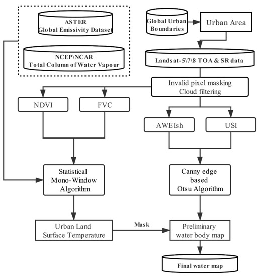
Figure 2.
Flowchart for extracting urban surface water using the automatic urban surface water mapping (AUSWM) method based on Google Earth Engine.
2.3.5. Accuracy Assessment
The following four indicators were used to evaluate the accuracy of the algorithm of AUSWM in urban water body mapping, namely: overall accuracy, Kappa coefficient, producer’s accuracy, and user’s accuracy [26,49]. To verify the differences in the LST of low- or high-reflection objects and water bodies, 720 random sample points were selected, and each category had 240 sample points.
The overall accuracy refers to the percentage of the number of pixels correctly classified as the number of total pixels (Equation (3)). The number of correctly classified pixels in remote sensing classification is arranged along the diagonal of a confusion matrix:
where Stotal represents the number of pixels correctly classified, and n represents the total number of sample points in accuracy assessment.
The producer’s accuracy is also known as “cartographic accuracy.” It represents the percentage between the number of pixels (diagonal values) in the entire image that the classifier correctly classifies into class A and the total number of true references of class A (i.e., the sum of class A columns in the confusion matrix) (Equation (4)). The user’s accuracy represents the degree of matching between the remote-sensing classification and the actual test data (Equation (5)).
where TP is the number of samples correctly classified into water points, FP represents the sample number of water points that were misclassified as non-water points, and FN represents the sample number of non-water points that were misclassified as water points.
The Kappa coefficient is calculated from a confusion matrix, and its value ranges from −1 to 1 (Equation (6)). Generally, the value of Kc is greater than 0.
where n is the total number of pixels, Sii means the diagonal value of the i-th confusion matrix, r is the number of rows of the confusion matrix, and Sy and Sz represent the sum of the observed values of the i-th row and column, respectively.
3. Results
3.1. Accuracy Assessment
3.1.1. Optimal Time for Calculating LST
Urban LST varies seasonally; therefore, an appropriate season is essential to be selected to eliminate non-water information. Here, the best-quality remote-sensing images were selected for each season: spring (March–May), summer (June–August), autumn (September–November), and winter (December–February) to distinguish urban surface water bodies and other objects in the urban area of Zhengzhou City (Figure 3).
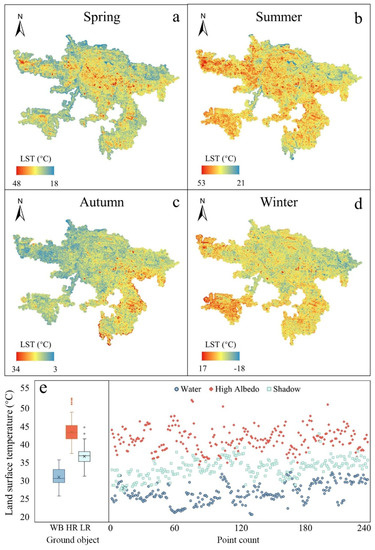
Figure 3.
Land surface temperature (LST) inversion in different seasons: (a) spring, (b) summer, (c) autumn, and (d) winter, and (e) temperature differences of sample points of three urban coverage types: water bodies and low- and high-reflection objects. The abbreviations of WB, HR, and LR in the figure represent water bodies, high-reflectance, and low-reflectance ground objects, respectively.
The average LST of water bodies and low- and high-reflection objects, together with the differences between them, are listed in Table 2. The largest LST difference between water bodies and high-reflection surfaces was in summer, followed by spring, autumn, and winter. The largest LST difference between water bodies and low-reflection objects (e.g., building shadows, black roads, and roofs) also appeared in summer, followed by spring, autumn, and winter. It indicates that LST data obtained in summer are most suitable for noise elimination, followed by those in spring; it is not appropriate to use remote-sensing image inversion of LST data for autumn and winter.
Table 2.
Average LST of different objects in all four seasons.
3.1.2. Accuracy Assessment of Urban Surface Water Body Mapping
Landsat synthetic images of Zhengzhou from April 2020 to September 2020 were used to generate the water body maps by using three kinds of algorithms, namely: AWEIsh, AWEIsh ∩ USI, and AUSWM. The random-sampling method and Sentinel-2A false-color synthetic images were used to validate the accuracies of the resultant water body maps. For each kind of water body map, a total of 750 sample points (350 ones for water and 400 ones for non-water) were randomly selected and interpreted to calculate the confusion matrix for accuracy assessment (Figure 4).
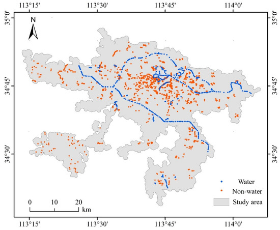
Figure 4.
Spatial distributions of the randomly selected samples for accuracy verification of the annual maps of urban surface water bodies in Zhengzhou from 1990 to 2020.
Water noise in the urban area of Zhengzhou City was attributable mainly to industrial plant areas and the eastern and western suburbs (Figure 5). There were many noises in the water body information extracted using the two algorithms of AWEIsh and AWEIsh ∩ USI, especially in the vicinity of Ruyi Lake and Beilong Lake (Figure 5b,c) and where the surface environment was very complex (e.g., the dense landscape of lakes, rivers, green spaces, low-reflection roads, and high-reflection industrial areas). However, after superimposing the LST data, the noise was eliminated effectively (Figure 5d).
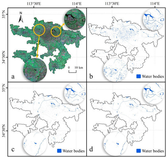
Figure 5.
Optimization effect on urban water body extraction: (a) Sentinel-2A false-color synthetic image of the study area in 2020, (b) AWEIsh with automatic threshold extraction, (c) AWEIsh ∩ USI extraction results, and (d) AUSWM extraction results.
Overall, the LST showed satisfactory performance in removing low- or high-reflection objects with LST higher or lower than that of urban water bodies. The OA of the resultant maps of surface water bodies from the algorithm of AWEIsh increased from 77.47% to 84.8% when using the AWEIsh ∩ USI method; however, the AUSWM with the combination of the AWEIsh ∩ USI method and LST achieved the higher accuracy of 96.0%. Meanwhile, the Kappa coefficient correspondingly increased from 0.55 for the AWEIsh method, to 0.70 for the AWEIsh ∩ USI method, and finally to 0.92 for the AUSWM (Table 3).
Table 3.
Urban surface water areas and accuracies derived from multi-source and multi-resolution remote sensing images.
3.2. Performance Comparison of Various Water-Body-Mapping Methods
For further comparison of the performances of different methods, five commonly used water indexes were considered and adopted, namely: LSWI, NDWI, MNDWI, AWEIsh, and USI. Two typical regions (orange rectangles in Figure 6 and Figure 7) in the urban area of Zhengzhou City were selected to conduct the comparison of the performances of water body mapping of different methods. As can be seen, the resultant water body maps from different water indexes and thresholds varied greatly (Figure 6 and Figure 7). There were a significant number of noises in the water body maps from LSWI with a threshold of lower than 0.2. Although the shadows of ground objects substantially decreased in the water body maps from NDWI with the threshold of higher than 0.15, some rivers still have not been detected. In terms of the results of MNDWI, more noises were still contained in the water body maps at that threshold interval. In the AWEIsh results, noises were largely eliminated at the threshold of 0.15, but some water bodies were missed. The performance of the USI method was relatively stable, and the resultant water body map was most reliable when the threshold was set to 0.15. The water bodies obtained using the AUSWM method are shown in Figure 6c. By combining the results of the AWEIsh, USI, and LST, the AUSWM approach significantly improved the accuracy.
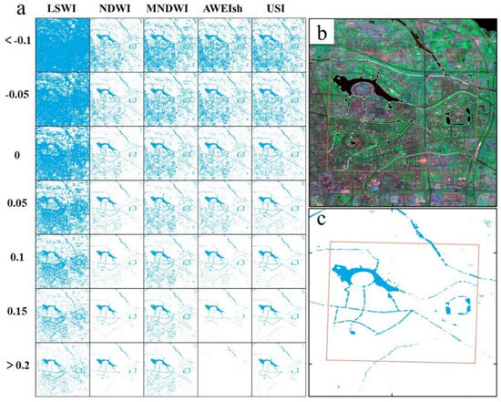
Figure 6.
Experimental area A for comparison of water body extraction methods: (a) extraction results using different water body indexes with different thresholds, (b) real water profile, and (c) results obtained using the automatic urban surface water mapping (AUSWM) method.
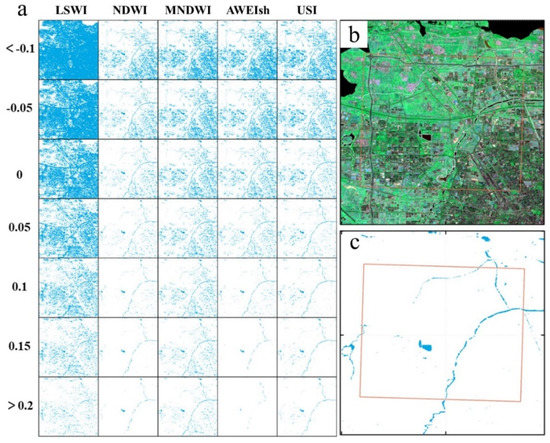
Figure 7.
Experimental area B for comparison of water body extraction methods: (a) extraction results using different water body indexes with different thresholds, (b) real water profile, and (c) results obtained using the automatic urban surface water mapping (AUSWM) method.
3.3. Temporal Changes in Urban Surface Water Bodies in Zhengzhou
High-quality satellite imagery is important for water extraction. Remote-sensing images of Zhengzhou have at least 10 effective observation pixels each year, which ensures the quality of water body change monitoring at the interannual scale. In this study, a total of 730 Landsat images (Landsat 5, 7, and 8) were used for urban surface water extraction in Zhengzhou City (Figure 8).
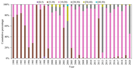
Figure 8.
Cumulative percentage of Landsat pixels with the good-quality observations of [0,5), [5,10), [10,20), [20,30), [30,40), and [40,50), respectively, in Zhengzhou City during 1990–2020.
The trend in surface water area was different in the urban area of Zhengzhou City during different periods. Specifically, the changes in surface water area were not obvious during 1990—2017 and the trend was not statistically significant. Then, surface water area continuously and significantly (R2 = 0.93, p < 0.01) increased from 11.5 km2 in 2008 to 48.7 km2 in 2020 at a rate of 3.0 km2/yr (Figure 9). Spatially, regular water bodies appeared in northern regions of the city during 1990–1995, but they began to decrease substantially after 1995. After 2005, the Dongfeng Canal and Ruyi Lake gradually formed and the water area in Zhengzhou began to increase obviously. Since 2008, water bodies such as Beilong Lake, Longzi Lake, the main canal of the South-to-North Water Diversion Project, Wei River, and Jialu River have gradually appeared on the water map. Consequently, in 2020, the water area in Zhengzhou was nearly 4 times that in 1990 (Figure 10).
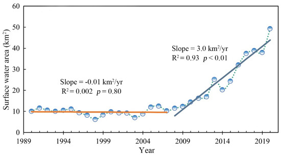
Figure 9.
Change in total surface water area in Zhengzhou during 1990–2020.
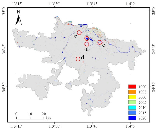
Figure 10.
Spatial patterns of changes in surface water bodies in Zhengzhou City from 1990 to 2020 (a: Dongfeng River and Ruyi Lake, b: Beilong Lake, c: Longzi Lake, d: South-to-North Water Diversion Project transfer canal, and e: Jialu River).
4. Discussion
4.1. Comparison with Previous Studies
On a global scale, Pekel et al. [21] and Ji et al. [4] generated the long-term surface water body maps using all the available Landsat and MODIS data, respectively. Other studies [44,45] performed water body mapping and change analyses on regional (e.g., North China Plain) and national scales (e.g., the United States, China, and Mongolia). However, in comparison with the natural environment, the urban environment is particularly complex, and urban surface water is especially affected by elements of the artificial environment, such as low- and high-reflection objects that cause noise [39]. Therefore, some conventional remote-sensing extraction methods are unsuitable for mapping urban surface water bodies. Some earlier studies tried to construct new methods for the extraction of urban surface water [27,39]. Although these methods are effective in removing the shadow of urban buildings, they do not consider the interference from high-reflection ground objects and dark asphalt surfaces in the urban environment, and the accuracy of water extraction is largely dependent on the selection of appropriate thresholds [31]. Corresponding to the two experimental areas shown in Figure 6 and Figure 7, it can be seen that although the threshold methods with the five water indexes have certain merits, it is not easy to determine suitable thresholds (Figure 11).
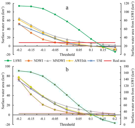
Figure 11.
Water areas from five water indexes with various thresholds: (a) experimental area A and (b) experimental area B. The abbreviations of LSWI, NDWI, MNDWI, AWEIsh, and USI in the figure represent Land Surface Water Index, Normalized Difference Water Index, Modified Normalized Difference Water Index, Automated Water Extraction Index for shadow, and Urban Shadow Index, respectively.
The AUSWM method proposed in this study effectively resolves the problem of noise interference in urban water body extraction. The new method was supported by spectral theory and LST differences between urban surface water bodies and other urban surfaces. In terms of spectra, the bright and dark values of water bodies and other surfaces can show clear differences in multiple bands [50]. However, the differences between water bodies and other objects are not obvious in thermal infrared bands, indicating that the digital number values of thermal infrared bands cannot effectively distinguish low- and high-reflection objects from water bodies (Figure 12). Considering the obvious LST differences between water bodies and other surfaces [1], especially in summer (Figure 3), the LST is very suitable for inclusion in the construction of an urban surface water extraction method.
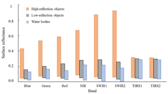
Figure 12.
Value distribution of sample points of high-reflection ground objects, shadows of buildings, and water bodies in Landsat-8 surface reflectance data.
4.2. Scale Effect of Remote-Sensing Images with Different Spatial Resolution
In the same region and at the same time, different spatial resolutions will lead to inconsistencies in the inversion of surface parameters using remote-sensing data [51]. In this study, 30 m-resolution remote-sensing images were used as the data source for urban surface water body mapping. In this process, the water body area will inevitably be affected by the scale effect. For experimental areas A and B (red rectangles in Figure 13a and Figure 14a), three remote sensing images from Sentinel-2A (10 m spatial resolution), Landsat-8 (30 m spatial resolution), and MODIS (250 m spatial resolution) acquired at similar times were used as data sources for water extraction. The Sentinel-2A images were resampled to resolutions of 50 and 100 m. Then, the water area extracted from the above remote-sensing images with five different resolutions was calculated to assess the area loss caused by the scale effect (Table 3). The results showed that the water area calculated using the Sentinel-2A 10 m spatial resolution image had the highest accuracy, with a relative loss of water area of lower than 2%. The accuracy achieved using the Landsat-8 30m-resolution image was higher than 93%, while the average accuracy achieved using the Sentinel-2A 50m-resolution image was lower than 83%, although the resolution differences all are 20 m. Therefore, a resolution of 30 m could represent a critical point for urban surface water extraction, and the area extracted using images with coarser resolution will decrease sharply. Of course, the proportion of small urban water bodies will be different in different cities and regions [52,53].
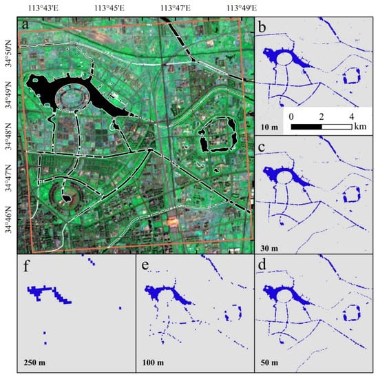
Figure 13.
Scale effect in experimental area A: (a) white lines in remote-sensing image indicate real surface water boundaries, (b) water area extracted using Sentinel-2A 10m-resolution data, (c) water area extracted using Landsat-8 30m-resolution data, (d) water area resampled to 50 m from Sentinel-2A 10m-resolution data, (e) water area resampled to 100 m from Sentinel-2A 10m-resolution data, and (f) water area extracted using MODIS 250-resolution data.
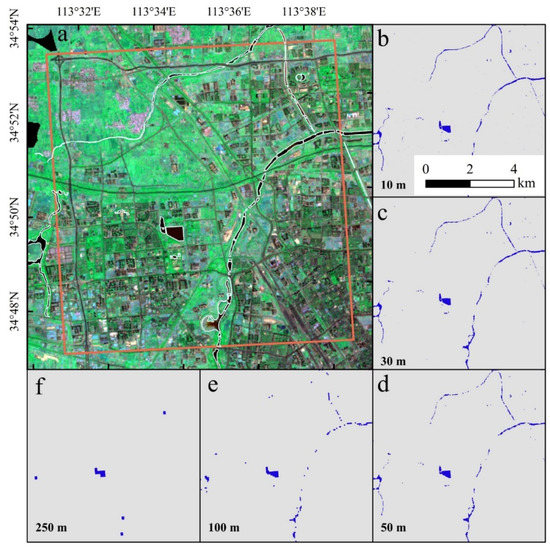
Figure 14.
Scale effect in experimental area B: (a) white lines in remote sensing image indicate real surface water boundaries, (b) water area extracted using Sentinel-2A 10m-resolution data, (c) water area extracted using Landsat-8 30m-resolution data, (d) water area resampled to 50 m from Sentinel-2A 10m-resolution data, (e) water area resampled to 100 m from Sentinel-2A 10m-resolution data, and (f) water area extracted using MODIS 250 m resolution data.
4.3. Uncertainties and Limitations in This Study
Although the currently proposed method of urban surface water body mapping achieved the satisfied accuracies higher than 96.0% and could contribute to the progress of research related to the monitoring of the dynamics of urban surface water resources, it is notable that some uncertainties and limitations remain in the approach in this study. Firstly, considering the smaller sizes of surface water bodies in the urban areas, water body mapping using Landsat data with the spatial resolution of 30 m could miss some water bodies with sizes smaller than 30 m × 30 m [44,45]. Therefore, it is inevitable that there are some errors between the annual areas of urban surface water bodies and the true values by using time series Landsat data. Secondly, some pixels of urban shadows may remain in the resultant maps of surface water bodies after shadow filtering, which might bring some uncertainties to the accuracies of urban surface water body mapping results. Finally, there are some differences between LST inversion and the true temperature; we have to recognize that the uncertainties brought by the accuracies of LST inversion might have led to some errors in the resultant water body maps. In addition, we have to acknowledge that the current approach can only detect surface water bodies; the wide application of the approach in mapping and monitoring the variations in urban wetlands should be improved by thoroughly considering the seasonality of the mixes of water and vegetation [44].
5. Conclusions
Mapping and monitoring the dynamics of surface water bodies are critical to the urban ecosystem and environmental management. However, the influence of noise from complex urban environments is the principal difficulty in mapping urban surface water bodies using remote-sensing techniques. In this study, we put forward the automatic urban surface water mapping (AUSWM) approach by introducing LST using all the available Landsat data and the Google Earth Engine cloud computing platform. The accuracy of the resultant maps of urban surface water bodies in Zhengzhou City by using this method reached 96.0%. Subsequent multi-annual dynamic analyses showed that the total water area in Zhengzhou City changed slowly during 1990–2007 but increased substantially since 2008. However, considering the limitation of the 30 m spatial resolution of the source imagery, the results might neglect or underestimate the area of small urban water bodies. This study suggested that the AUSWM method can effectively eliminate the influence of noise from low- and high-reflection objects in urban surface water body mapping and can be applied to the rapid, accurate, and long-term monitoring of urban surface water bodies over a large region.
Author Contributions
Conceptualization, Y.C., N.L. and J.D.; methodology, Y.C., Y.F., J.D. and Y.Z.; validation, X.L. and Z.S.; formal analysis, Y.F.; data curation, X.L. and Z.S.; writing—original draft preparation, Y.C., Y.F. and N.L.; writing—review and editing, Y.C., J.D. and Y.Z. All authors have read and agreed to the published version of the manuscript.
Funding
This research was funded by the National Key Research and Development Program of China, grant number 2021YFE0106700; National Natural Science Foundation of China, grant number 42071415; Outstanding Youth Foundation of Henan Natural Science, grant number 202300410049.
Acknowledgments
The authors would like to thank Tsinghua University for providing the Global Urban Boundaries vector data and the National Centers for Environmental Prediction and National Center for Atmospheric Research for providing the total column of water vapor data.
Conflicts of Interest
The authors declare no conflict of interest.
References
- Xue, Z.; Hou, G.; Zhang, Z.; Lyu, X.; Jiang, M.; Zou, Y.; Shen, X.; Wang, J.; Liu, X. Quantifying the cooling-effects of urban and peri-urban wetlands using remote sensing data: Case study of cities of Northeast China. Landsc. Urban Plan. 2019, 182, 92–100. [Google Scholar] [CrossRef]
- Xie, H.; Luo, X.; Xu, X.; Pan, H.; Tong, X. Automated subpixel surface water mapping from heterogeneous urban environments using Landsat 8 OLI imagery. Remote Sens. 2016, 8, 584. [Google Scholar] [CrossRef]
- Feng, M.; Sexton, J.O.; Channan, S.; Townshend, J.R. A global, high-resolution (30-m) inland water body dataset for 2000: First results of a topographic–spectral classification algorithm. Int. J. Digit. Earth 2016, 9, 113–133. [Google Scholar] [CrossRef]
- Ji, L.; Gong, P.; Wang, J.; Shi, J.; Zhu, Z. Construction of the 500 m resolution daily global surface water change database (2001–2016). Water Resour. Res. 2018, 54, 10270–10292. [Google Scholar] [CrossRef]
- Yang, X.; Zhao, S.; Qin, X.; Zhao, N.; Liang, L. Mapping of urban surface water bodies from Sentinel-2 MSI imagery at 10 m resolution via NDWI-based image sharpening. Remote Sens. 2017, 9, 596. [Google Scholar] [CrossRef]
- DeVries, B.; Huang, C.; Armston, J.; Huang, W.; Jones, J.W.; Lang, M.W. Rapid and robust monitoring of flood events using Sentinel-1 and Landsat data on the Google Earth Engine. Remote Sens. Environ. 2020, 240, 111664. [Google Scholar] [CrossRef]
- Markert, K.N.; Markert, A.M.; Mayer, T.; Nauman, C.; Haag, A.; Poortinga, A.; Bhandari, B.; Thwal, N.S.; Kunlamai, T.; Chishtie, F. Comparing sentinel-1 surface water mapping algorithms and radiometric terrain correction processing in southeast asia utilizing google earth engine. Remote Sens. 2020, 12, 2469. [Google Scholar] [CrossRef]
- Yang, X.; Chen, Y.; Wang, J. Combined use of Sentinel-2 and Landsat 8 to monitor water surface area dynamics using Google Earth Engine. Remote Sens. Lett. 2020, 11, 687–696. [Google Scholar] [CrossRef]
- Wang, J.; Ding, J.; Li, G.; Liang, J.; Yu, D.; Aishan, T.; Zhang, F.; Yang, J.; Abulimiti, A.; Liu, J. Dynamic detection of water surface area of Ebinur Lake using multi-source satellite data (Landsat and Sentinel-1A) and its responses to changing environment. CATENA 2019, 177, 189–201. [Google Scholar] [CrossRef]
- Fisher, A.; Flood, N.; Danaher, T. Comparing Landsat water index methods for automated water classification in eastern Australia. Remote Sens. Environ. 2016, 175, 167–182. [Google Scholar] [CrossRef]
- Li, M.; Stein, A.; Bijker, W.; Zhan, Q. Urban land use extraction from Very High Resolution remote sensing imagery using a Bayesian network. ISPRS J. Photogramm. Remote Sens. 2016, 122, 192–205. [Google Scholar] [CrossRef]
- Yang, X.; Qin, Q.; Grussenmeyer, P.; Koehl, M. Urban surface water body detection with suppressed built-up noise based on water indices from Sentinel-2 MSI imagery. Remote Sens. Environ. 2018, 219, 259–270. [Google Scholar] [CrossRef]
- Chen, F.; Chen, X.; Van de Voorde, T.; Roberts, D.; Jiang, H.; Xu, W. Open water detection in urban environments using high spatial resolution remote sensing imagery. Remote Sens. Environ. 2020, 242, 111706. [Google Scholar] [CrossRef]
- Delgado, R.C.; Sediyama, G.C.; Costa, M.H.; Soares, V.P.; Andrade, R.G. Spectral classification of planted area with sugarcane through the decision tree. Eng. Agrícola 2012, 32, 369–380. [Google Scholar] [CrossRef]
- Crasto, N.; Hopkinson, C.; Forbes, D.; Lesack, L.; Marsh, P.; Spooner, I.; Van Der Sanden, J. A LiDAR-based decision-tree classification of open water surfaces in an Arctic delta. Remote Sens. Environ. 2015, 164, 90–102. [Google Scholar] [CrossRef]
- Acharya, T.D.; Lee, D.H.; Yang, I.T.; Lee, J.K. Identification of water bodies in a Landsat 8 OLI image using a J48 decision tree. Sensors 2016, 16, 1075. [Google Scholar] [CrossRef]
- Yang, G.; Fang, S. Improving remote sensing image classification by exploiting adaptive features and hierarchical hybrid decision trees. Remote Sens. Lett. 2017, 8, 156–164. [Google Scholar] [CrossRef]
- Cortes, C.; Vapnik, V. Support-vector networks. Mach. Learn. 1995, 20, 273–297. [Google Scholar] [CrossRef]
- Mountrakis, G.; Im, J.; Ogole, C. Support vector machines in remote sensing: A review. ISPRS J. Photogramm. Remote Sens. 2011, 66, 247–259. [Google Scholar] [CrossRef]
- Li, N.; Zhu, X.; Pan, Y.; Zhan, P. Optimized SVM based on artificial bee colony algorithm for remote sensing image classification. J. Remote Sens 2018, 22, 559–569. [Google Scholar]
- Pekel, J.-F.; Cottam, A.; Gorelick, N.; Belward, A.S. High-resolution mapping of global surface water and its long-term changes. Nature 2016, 540, 418–422. [Google Scholar] [CrossRef] [PubMed]
- Breiman, L. Random forests. Mach. Learn. 2001, 45, 5–32. [Google Scholar] [CrossRef]
- Kim, J.; Popescu, S.C.; Lopez, R.R.; Wu, X.B.; Silvy, N.J. Vegetation mapping of No Name Key, Florida using lidar and multispectral remote sensing. Int. J. Remote Sens. 2020, 41, 9469–9506. [Google Scholar] [CrossRef]
- Isikdogan, F.; Bovik, A.C.; Passalacqua, P. Surface water mapping by deep learning. IEEE J. Sel. Top. Appl. Earth Obs. Remote Sens. 2017, 10, 4909–4918. [Google Scholar] [CrossRef]
- Zhang, P.; Chen, L.; Li, Z.; Xing, J.; Xing, X.; Yuan, Z. Automatic extraction of water and shadow from SAR images based on a multi-resolution dense encoder and decoder network. Sensors 2019, 19, 3576. [Google Scholar] [CrossRef]
- Yang, X.; Qin, Q.; Yésou, H.; Ledauphin, T.; Koehl, M.; Grussenmeyer, P.; Zhu, Z. Monthly estimation of the surface water extent in France at a 10-m resolution using Sentinel-2 data. Remote Sens. Environ. 2020, 244, 111803. [Google Scholar] [CrossRef]
- Wu, W.; Li, Q.; Zhang, Y.; Du, X.; Wang, H. Two-step urban water index (TSUWI): A new technique for high-resolution mapping of urban surface water. Remote Sens. 2018, 10, 1704. [Google Scholar] [CrossRef]
- Verpoorter, C.; Kutser, T.; Tranvik, L. Automated mapping of water bodies using Landsat multispectral data. Limnol. Oceanogr. Methods 2012, 10, 1037–1050. [Google Scholar] [CrossRef]
- Xu, T.; Tan, Z.; Yan, X. Extraction techniques of urban water bodies based on object-oriented. Geospat. Inf. 2010, 8, 64–66. [Google Scholar]
- Zhang, T.; Yang, X.; Hu, S.; Su, F. Extraction of coastline in aquaculture coast from multispectral remote sensing images: Object-based region growing integrating edge detection. Remote Sens. 2013, 5, 4470–4487. [Google Scholar] [CrossRef]
- Zhou, Y.; Dong, J. Review on monitoring open surface water body using remote sensing. J. Geogr. Inf. Sci 2019, 21, 1768–1778. [Google Scholar]
- Crist, E.P. A TM tasseled cap equivalent transformation for reflectance factor data. Remote Sens. Environ. 1985, 17, 301–306. [Google Scholar] [CrossRef]
- McFeeters, S.K. The use of the Normalized Difference Water Index (NDWI) in the delineation of open water features. Int. J. Remote Sens. 1996, 17, 1425–1432. [Google Scholar] [CrossRef]
- Han-Qiu, X. A study on information extraction of water body with the modified normalized difference water index (MNDWI). J. Remote Sens. 2005, 9, 589–595. [Google Scholar]
- Xu, H. Modification of normalised difference water index (NDWI) to enhance open water features in remotely sensed imagery. Int. J. Remote Sens. 2006, 27, 3025–3033. [Google Scholar] [CrossRef]
- Xiao, X.; Boles, S.; Frolking, S.; Salas, W.; III, B.M.; Li, C.; He, L.; Zhao, R. Observation of flooding and rice transplanting of paddy rice fields at the site to landscape scales in China using VEGETATION sensor data. Int. J. Remote Sens. 2002, 23, 3009–3022. [Google Scholar] [CrossRef]
- Chandrasekar, K.; Sesha Sai, M.; Roy, P.; Dwevedi, R. Land Surface Water Index (LSWI) response to rainfall and NDVI using the MODIS Vegetation Index product. Int. J. Remote Sens. 2010, 31, 3987–4005. [Google Scholar] [CrossRef]
- Menarguez, M. Global Water Body Mapping from 1984 to 2015 Using Global High Resolution Multispectral Satellite Imagery; University of Oklahoma: Norman, OK, USA, 2015. [Google Scholar]
- Feyisa, G.L.; Meilby, H.; Fensholt, R.; Proud, S.R. Automated Water Extraction Index: A new technique for surface water mapping using Landsat imagery. Remote Sens. Environ. 2014, 140, 23–35. [Google Scholar] [CrossRef]
- Wang, Y.; Zhan, Q.; Ouyang, W. How to quantify the relationship between spatial distribution of urban waterbodies and land surface temperature? Sci. Total Environ. 2019, 671, 1–9. [Google Scholar] [CrossRef]
- Li, X.; Gong, P.; Zhou, Y.; Wang, J.; Bai, Y.; Chen, B.; Hu, T.; Xiao, Y.; Xu, B.; Yang, J. Mapping global urban boundaries from the global artificial impervious area (GAIA) data. Environ. Res. Lett. 2020, 15, 094044. [Google Scholar] [CrossRef]
- Foga, S.; Scaramuzza, P.L.; Guo, S.; Zhu, Z.; Dilley Jr, R.D.; Beckmann, T.; Schmidt, G.L.; Dwyer, J.L.; Hughes, M.J.; Laue, B. Cloud detection algorithm comparison and validation for operational Landsat data products. Remote Sens. Environ. 2017, 194, 379–390. [Google Scholar] [CrossRef]
- Roy, D.P.; Kovalskyy, V.; Zhang, H.; Vermote, E.F.; Yan, L.; Kumar, S.; Egorov, A. Characterization of Landsat-7 to Landsat-8 reflective wavelength and normalized difference vegetation index continuity. Remote Sens. Environ. 2016, 185, 57–70. [Google Scholar] [CrossRef] [PubMed]
- Zhou, Y.; Dong, J.; Cui, Y.; Zhou, S.; Li, Z.; Wang, X.; Deng, X.; Zou, Z.; Xiao, X. Rapid surface water expansion due to increasing artificial reservoirs and aquaculture ponds in North China Plain. J. Hydrol. 2022, 608, 127637. [Google Scholar] [CrossRef]
- Zhou, Y.; Dong, J.; Xiao, X.; Liu, R.; Zou, Z.; Zhao, G.; Ge, Q. Continuous monitoring of lake dynamics on the Mongolian Plateau using all available Landsat imagery and Google Earth Engine. Sci. Total Environ. 2019, 689, 366–380. [Google Scholar] [CrossRef] [PubMed]
- Crist, E.P.; Cicone, R.C. A Physically-Based Transformation of Thematic Mapper Data-The TM Tasseled Cap. IEEE Trans. Geosci. Remote Sens. 1984, 22, 256–263. [Google Scholar] [CrossRef]
- Ermida, S.L.; Soares, P.; Mantas, V.; Göttsche, F.-M.; Trigo, I.F. Google Earth Engine Open-Source Code for Land Surface Temperature Estimation from the Landsat Series. Remote Sens. 2020, 12, 1471. [Google Scholar] [CrossRef]
- Donchyts, G.; Schellekens, J.; Winsemius, H.; Eisemann, E.; Van de Giesen, N. A 30 m resolution surface water mask including estimation of positional and thematic differences using landsat 8, srtm and openstreetmap: A case study in the Murray-Darling Basin, Australia. Remote Sens. 2016, 8, 386. [Google Scholar] [CrossRef]
- Li, X.; Yeh, A.G.O. Accuracy improvement of land use change detection using principal components analysis: A case study in the Pearl River Delta. J. Remote Sens. 1997, 1, 282–289. [Google Scholar]
- Sun, G.; Huang, H.; Weng, Q.; Zhang, A.; Jia, X.; Ren, J.; Sun, L.; Chen, X. Combinational shadow index for building shadow extraction in urban areas from Sentinel-2A MSI imagery. Int. J. Appl. Earth Obs. Geoinf. 2019, 78, 53–65. [Google Scholar] [CrossRef]
- Li, X.; Wang, Y. Prospects on future developments of quantitative remote sensing. Acta Geogr. Sin. 2013, 68, 1163–1169. [Google Scholar]
- Shao, Z.; Fu, H.; Li, D.; Altan, O.; Cheng, T. Remote sensing monitoring of multi-scale watersheds impermeability for urban hydrological evaluation. Remote Sens. Environ. 2019, 232, 111338. [Google Scholar] [CrossRef]
- Wang, X.X.; Xiao, X.M.; Zou, Z.H.; Dong, J.W.; Qin, Y.W.; Doughty, R.B.; Menarguez, M.A.; Chen, B.Q.; Wang, J.B.; Ye, H.; et al. Gainers and losers of surface and terrestrial water resources in China during 1989–2016. Nat Commun. 2020, 11, 3471. [Google Scholar] [CrossRef] [PubMed]


Publisher’s Note: MDPI stays neutral with regard to jurisdictional claims in published maps and institutional affiliations. |
© 2022 by the authors. Licensee MDPI, Basel, Switzerland. This article is an open access article distributed under the terms and conditions of the Creative Commons Attribution (CC BY) license (https://creativecommons.org/licenses/by/4.0/).