1. Introduction
With the increasing applications of computer vision technology in various engineering fields [
1,
2,
3,
4,
5,
6,
7,
8,
9,
10,
11], hyperspectral images (HSIs) have proved to obtain more helpful information than RGB images. Hyperspectral images contain the reflectance of objects or scenes in different spectral bands, usually ranging from several dozens to hundreds, even outside the visible spectrum (e.g., in the ultraviolet or infrared spectrum). Compared with traditional RGB images with increased spectral range and resolution, HSIs provide much richer information, which has been widely used in cultural heritage [
1,
2], medical diagnosis [
3], remote sensing [
4], food quality inspection [
5], color quality control [
6], and various computer vision tasks, such as face recognition, object tracking, and image classification [
7,
8,
9].
Due to the growing need for HSIs, various hyperspectral imaging systems (HISs) have been developed in the last several decades. The first HISs, such as NASA’s airborne visible/infrared imaging spectrometer (AVIRIS) [
12], employed a prism to disperse the reflected light and a linear array detector to record the reflected light. This kind of HISs can acquire images with high spatial/spectral resolution in “whisk broom” imaging mode, but image acquisition is time-consuming since they adopt the point-scanning method. Afterwards, “push broom” HISs, such as NASA’s advanced land imager (ALI) [
13], and “staring” HISs, often used in microscopy or other lab applications, have been developed. With a scan lens and an entrance slit, “push broom” HISs use a prism-grating-prism to split the light and can scan one line at a time; “staring” HISs use continuously changeable narrow bandpass filters in front of a matrix detector and can capture the image at one wavelength at a given time. Obviously, the latter two have relatively fast speed of scanning, but their temporal resolutions are still not high enough for dynamic scenes. Thus, many non-scanning, snapshot HISs have been designed, including computed tomographic imaging spectrometry (CTIS), fiber-reformatting imaging spectrometry (FRIS), and coded aperture snapshot spectral imaging (CASSI) [
14]. Unfortunately, as the total number of voxels cannot exceed the total number of pixels on the CCD camera, these HISs involve a trade-off between spatial and spectral resolution [
15].
As aforementioned, HISs to directly acquire HSIs have disadvantages either in temporal resolution or in spatial resolution. In recent years, hyperspectral reconstruction from RGB images has become a very active research topic. A large number of methods have been proposed to reconstruct hyperspectral information using only RGB cameras [
16,
17,
18,
19,
20,
21,
22,
23,
24,
25,
26,
27,
28,
29,
30,
31,
32,
33]. In general, these methods fall into three branches: traditional, machine learning, and deep learning methods. Traditional methods include classical methods on the basis of Wiener estimation, pseudo-inverse estimation, or principal component analysis, and their various modifications, such as adaptive Wiener estimation [
16], regularized local linear models [
17], sequential weighted nonlinear regression models [
18], and so on. Classical methods are simple and straight but not very accurate. Modified methods tend to adaptively select or weigh training samples, which enhances hyperspectral reconstruction accuracy, but are not portable and can be time-consuming. Therefore, it is hard for these traditional methods to be applied in real tasks. Fortunately, machine learning-based methods compute hyperspectral data, which makes acquisition of spectral data fast. Shallow learning models such as RBF networks [
19,
20], dictionary learning-based sparse coding [
21,
22], and manifold-based mapping [
23] are typical machine learning-based methods. Nevertheless, the expression capacity of handcrafted prior models learned by these methods is so limited that the reconstructed spectra are not very accurate. In recent years, deep learning methods have been used for hyperspectral reconstruction and have achieved remarkable success. Compared to machine learning methods, deep learning methods are capable of automatically extracting high-level features and have a better generalization ability. Convolutional neural networks (CNNs) [
24,
25,
26,
27,
28,
29,
30,
31] and generative adversarial networks (GANs) [
32,
33] have been developed for hyperspectral reconstruction.
Though considerable progress has been made for hyperspectral reconstruction, challenges remain in deep learning-based models as noted below: (1) when using dense skip connections, the feature of each layer is propagated into all subsequent layers, resulting in a very wide network at the cost of reducing the depth of the network [
34]; (2) the commonly used non-local spatial attention involves big matrix multiplications, raising the cost of computation and memory requirement, thus hindering the frequent application in the network [
35]; (3) deep learning-based models for hyperspectral reconstruction neglect that the importance of different intermediate layers varies. To address these issues, we propose a densely residual network with dual attention (DRN-DA) for more powerful feature representation, which adequately enjoys the benefits of both the residual block [
36] and the dense block [
34]. In our proposed DRN-DA network, the basic building blocks are densely residual block (DRB) and densely residual attention block (DRAB). The difference between DRB and DRAB is that DRAB has channel attention (CA) and dual downsampling spatial attention (DDSA) to capture channel-wise and long-range spatial dependencies. Then, to reuse the features, the output features of DRB and DRAB are adaptively fused. Additionally, an adaptive multi-scale block (AMB) with larger receptive fields is used to process the features generated by the previous network. Extensive experiments demonstrate that the proposed DRN-DA network performs better when compared to the state-of-the-art methods.
In summary, the contributions of this paper are as follows:
We propose a novel model, named densely residual network with dual attention (DRN-DA), which enhances the representation ability of feature learning for hyperspectral reconstruction.
We propose a lightweight dense skip connection, where each layer is connected to the next layer rather than all the subsequent layers. Although this block is different from the classic DenseNet [
34], it also reuses features and eliminates gradient vanishing.
We propose a simple but effective non-local block named dual downsampling spatial attention (DDSA) to decrease the computation and memory consumption of the standard non-local block, which makes it feasible to insert multiple non-local blocks in the network for enhancing the performance.
To further improve the learning ability of the network, we introduce an adaptive fusion block (AFB) to adaptively reuse the features from different intermediate layers.
The remainder of this paper is organized as follows.
Section 2 briefly introduces the related work.
Section 3 illustrates the details of the proposed method. Experiment studies and discussion of results are given in
Section 4. Finally, the conclusion is drawn in
Section 5.
3. Methodology
In this section, we firstly introduce the network structure of DRN-DA, and then detail the densely residual attention block (DRAB), adaptive fusion block (AFB), and the adaptive multi-scale block (AMB).
Some basic nomenclature is first introduced before the proposed network is described in detail. Different convolutions are distinguished by superscript numbers. For example, denotes the function of a 1 × 1 convolutional layer, and represents the function of a 3 × 3 convolutional layer. Additionally, and denote the concatenation operation and PReLU activation function, respectively.
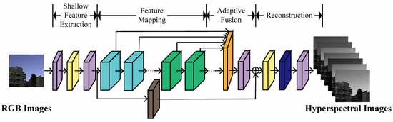
3.1. Network Architecture of DRN-DA
The overall architecture of DRN-DA is shown in
Figure 1. DRN-DA falls into four stages, including a shallow feature extraction stage, a feature mapping stage, an adaptive fusion stage, and a reconstruction stage. Let us denote
and
as the input and output of DRN-DA. Here, 3 or 31 is the band number,
N is the batch size,
H is the height, and
W is the width.
Firstly, we use two 3 × 3 convolutional layers with an activation function called a parametric rectified linear unit (PReLU) [
48] between them to extract the shallow features
from RGB input images
where
represents the shallow feature extraction function. Then, the shallow features
are fed to the feature mapping stage for higher-level feature extraction.
C is the channel number of the feature map. The procedure can be described as follows:
where
represents the feature mapping function, which consists of
DRBs and
DRABs.
is composed of a set of feature maps as
Then, in the adaptive fusion stage, the feature maps extracted by multiple DRBs and DRABs are adaptively fused. This procedure is expressed as
where
represents the fusion function described in
Section 3.3. At the end of the adaptive fusion stage, global residual learning is introduced to keep the network stable. For the identity mapping branch, a 5 × 5 convolutional layer is utilized to further process the shallow features. The global residual learning can be formulated as
In the final stage, the global feature representation
is reconstructed via a reconstruction module as follows:
where
and
are the reconstruction module and the function of the network of DRN-DA, respectively. The reconstruction module is composed of an adaptive multi-scale block (AMB) and a 3 × 3 convolutional layer. The AMB block has three branches with multiple scale convolutions, and corresponding weights can be automatically learned to make full use of more important representations. Finally, the convolutional layer is used to compress the dimension to
, which is the same as the dimension of the ground-truth HSIs.
3.2. Densely Residual Attention Block
As shown in
Figure 1, the backbone of the proposed network DRN-DA is stacked with multiple densely residual blocks (DRB) and densely residual attention blocks (DRAB). As the only difference between DRB and DRAB lies in that DRB does not incorporate attention mechanisms, while DRAB has them, here, only DRAB is described in detail. As shown in
Figure 1, DRAB consists of a lightweight dense connection and local residual learning. The lightweight dense connection is inspired by DenseNet [
34] to alleviate the vanishing-gradient problem and strengthen feature propagation. However, the feature maps are used as inputs into all subsequent layers in the original DenseNet, which results in the DenseNet becoming wider and wider with increasing depth. Therefore, here, a simplified densely connected network is developed to reduce the computation cost. The output of each multi-scale residual attention block (MRAB) is only used as the input into the following second MRAB. After the feature maps of two consecutive layers are concatenated, a 3 × 3 convolutional layer is added to reduce the dimension, which further lowers the width of the dense connection. The procedure of DRAB can be formulated as
where
,
,
, and
denote the input of the first, second, and third MRAB, and the feature map which is output from the third MRAB and processed via a convolutional layer, respectively;
is the function of MRAB.
As shown in
Figure 1, MRAB is composed of three subcomponents, namely multi-scale residual block (MRB), channel attention (CA), and dual downsampling spatial channel (DDSA). The features are processed by three branches: the first branch is stacked with three MRBs; the second branch consisting of CA is parallel to the second MRB; and the third branch consisting of DDSA is parallel to the second MRB as well. Both CA and DDSA work on the second MRB, and the feature maps are fused with concatenation and compression in the channel dimension. The procedure of MRAB is described by the following equations:
where
,
,
, and
denote the input of MRAB and the outputs of the first, second, and third MRB, respectively;
,
, and
represent the functions of MRB, CA and DDSA; ⊗ and ⊕ denote the element-wise multiplication and addition, respectively.
Next, we give more details on the multi-scale residual block (MRB), channel attention (CA), and dual downsampling spatial channel (DDSA).
3.2.1. Multi-Scale Residual Block
Since it has been proven that wider features before the activation layer of the residual block can exploit the multi-level features better [
49,
50], a multi-scale residual block (MRB) is used in the basic building block MRAB. Different from the MRB in [
50], a modified MRB is adopted. Inspired by Inception-V2 [
51], the 5 × 5 convolutional layer and the 7 × 7 convolutional layer in the multi-scale convolution block from [
50] are replaced by two 3 × 3 convolutional layers and three 3 × 3 convolutional layers, respectively. This strategy is adopted to reduce parameters as well as the computational time, but can make the stacked convolutions reach the same receptive fields as the convolutions in [
43]. Additionally, the activation function ReLU is replaced by PReLU to introduce more nonlinearity and accelerate convergence. The MRB in this work consists of several parts: a multi-scale convolution block, a PReLU activation function, a feature fusion bottleneck layer, a 3 × 3 convolution layer, and a local residual learning block (see
Figure 2).
Multi-Scale Convolution Block: The computations of the three paths in multi-scale convolution block are formulated as
where
,
,
, and
are the input of the multi-scale convolution block and the outputs of the first, second, and third paths;
,
,
,
,
, and
are the 3 × 3 convolutional layer in the first path, the first and second 3 × 3 convolutional layers in the second path, and the first, second, third 3 × 3 convolutional layers in the third path.
Feature Fusion: The feature maps output from three paths are concatenated and activated. As a result, 3 × C feature maps are generated. Then, a 1 × 1 convolutional layer is used to fuse the multi-scale features and compress the number of channels. Finally, a 3 × 3 convolutional layer is employed to extract spatial-wise features. This procedure of feature fusion can be formulated as
Local Residual Learning: considering that there are multiple convolutional layers in the above architecture, local residual learning is used to enhance the feature map. The final output feature map of MRB is given by
3.2.2. Channel Attention
In previous tasks, channel-wise attention has been proven to be efficient to select significant features [
29,
39,
40,
42,
43]. The channel attention in the MRAB architecture is the same as the SE layer [
39] shown in
Figure 3. First, the input feature
is compressed through a global average pooling and made into a global statistics vector
:
Next, two fully-connected (FC) layers are used to obtain a bottleneck. The first FC layer is a channel-reduction layer with reduction ratio r, and the second FC layer restores the number of channels. Between the two FC layers, a PRELU is used to increase the nonlinearity.
Finally, a sigmoid function is applied as a gating mechanism to acquire the channel statistics.
3.2.3. Dual Downsampling Spatial Attention
The non-local self-attention mechanism proposed by Wang [
35] can capture the long-range dependencies at all positions throughout the entire image. It has been used in various computer vision applications such as video classification and image recognition, and yields great improvement. However, the standard non-local network consumes a large amount of computational memory since each position’s signal is calculated on the whole image, and the computational cost is prohibitive when the image has a large size. Though region-level non-local modules [
42] and patch-level non-local modules [
29] reduce computational time to some extent, these methods are not efficient enough yet. To address this problem, modified non-local attention is developed in this work to model spatial correlation. In this attention block, a dual downsampling strategy is used to reduce the channel dimension and the size of the input image as illustrated in
Figure 4. Let
be the input feature map; then, three convolutions are used to convert
into three different feature maps,
,
, and
. Concretely, the three convolutions are in the size
, and the latter two convolutions have a stride with
t to downsample the image in size. This process can be expressed as
Next, the three feature maps are flattened to
,
, and
. Then, a spatial attention map is calculated through multiplying the transposed first feature map by the second feature map and normalized by a Softmax activation function as
where
denotes the Softmax function, and
is the spatial attention matrix. Subsequently, the feature map
is multiplied by the transposed
to acquire the weighted feature map
, which is formulated as
At last,
is reshaped to
and then recovered to the same channel dimension as the input feature map
by a 1 × 1 convolution. Therefore, the final output is obtained by
3.3. Adaptive Fusion Block
A traditional fusion structure integrates the hierarchical features from early layers to make full use of features from different levels [
28,
52]. However, most global fusion blocks treat different layers equally. This causes the network to omit more important information, and the quality of reconstructed image is reduced. Therefore, an efficient structure is developed to make the fusion block more effective. Taking the inter-layer relationships into account, in this work, an adaptive fusion block (AFB) is used to fuse the outputs of all DRBs and DRABs (see
Figure 1). Each output has an independent weight that is adaptively and automatically adjusted in [0, 1] according to the training loss. The features from different layers are weighted, concatenated, and fused by a convolution. Mathematically, the procedure can be formulated as
where
,
,
, and
are trainable weights representing weights of the first,
th DRB, the first and
th DRAB, respectively;
reduces the channel number.
3.4. Adaptive Multi-Scale Block
For a deep learning network, a larger receptive field usually brings the network better representative capability. In this work, at the tail of the proposed network DRN-DA, an AMB with larger receptive fields than the previous multi-scale convolution block in
Figure 2 is added to further improve the performance of the network as shown in
Figure 1. The AMB is comprised of three kinds of scale convolutions (see
Figure 5) with kernel sizes of 3 × 3, 5 × 5, and 7 × 7. After each convolution, the PReLU function is added to increase nonlinearity, and the other convolution with the same size is used to make the receptive field larger. The weight of each scale branch is automatically learned according to the training loss, which results in a trade-off between the reconstruction quality and parameters. The computational process of AMB can be formulated as
where
and
represent the input and the output of AMB, respectively; and
,
, and
are the weights of the three branches.


