Automatic Deployment of Convolutional Neural Networks on FPGA for Spaceborne Remote Sensing Application

Abstract

In recent years, convolutional neural network (CNN)-based algorithms have been widely used in remote sensing image processing and show tremendous performance in a variety of application fields. However, large amounts of data and intensive computations make the deployment of CNN-based algorithms a challenging problem, especially for the spaceborne scenario where resources and power consumption are limited. To tackle this problem, this paper proposes an automatic CNN deployment solution on resource-limited field-programmable gate arrays (FPGAs) for spaceborne remote sensing applications. Firstly, a series of hardware-oriented optimization methods are proposed to reduce the complexity of the CNNs. Secondly, a hardware accelerator is designed. In this accelerator, a reconfigurable processing engine array with efficient convolutional computation architecture is used to accelerate CNN-based algorithms. Thirdly, to bridge the optimized CNNs and hardware accelerator, a compilation toolchain is introduced into the deployment solution. Through the automatic conversion from CNN models to hardware instructions, various networks can be deployed on hardware in real-time. Finally, we deployed an improved VGG16 network and an improved YOLOv2 network on Xilinx AC701 to evaluate the effectiveness of the proposed deployment solution. The experiments show that with only 3.407 W power consumption and 94 DSP consumption, our solution achieves 23.06 giga operations per second (GOPS) throughput in the improved VGG16 and 22.17 GOPS throughput in the improved YOLOv2. Compared to the related works, the DSP efficiency of our solution is improved by 1.3–2.7×.

1. Introduction

Spaceborne remote sensing is a key component of remote sensing technology. Compared with ground remote sensing and airborne remote sensing, spaceborne remote sensing has the advantages of a large coverage area, a low cost per unit area of coverage, and frequent coverage of areas of interest [1]. Such advantages enable spaceborne remote sensing to obtain images with large coverage areas and high information density. Meanwhile, benefiting from the tremendous development in deep learning and computer vision, many convolutional neural network (CNN)-based methods have been proposed for remote sensing image processing and greatly improve the efficiency of extracting useful information from remote sensing images, thereby promoting the rapid development of scene classification and object detection based on spaceborne remote sensing images [2,3,4]. Therefore, spaceborne remote sensing is increasingly used in ship detection [5,6], cloud detection [7,8], land-cover classification [9,10], and other applications.

Traditional spaceborne remote-sensing processing systems process images on ground stations [11], which means the images have to be downloaded from the spacecraft. With the continuous growth of remote-sensing image data, such systems suffer from the low bandwidth and high latency of space–ground transmission links [12]. However, if CNN-based image processing is performed on the spacecraft, and only the extracted effective information is transmitted to the ground station, the processing latency of the system would be greatly reduced. Thus, many researchers focus on deploying the CNN-based methods on spaceborne platforms [13,14].

To achieve great performance and accuracy, many CNN models adopt deep and wide structures, resulting in intensive computations and great memory overheads. To address these issues, high-performance platforms such as graphics processing units (GPUs) are used widely in CNN training and inference [15,16]. However, the huge power consumption of GPUs limits their application in spaceborne scenarios [17]. To find a trade-off between power consumption and performance, many researchers conduct studies based on field-programmable gate arrays (FPGAs) and application-specific integrated circuits (ASICs). ASICs achieve high power efficiency and high performance due to their specific structure; however, their high costs and long development cycles are daunting issues [18]. FPGAs are programmable devices that allow customers to configure them by themselves. Due to their low-level power consumption and short iteration cycles, FPGAs are often used as efficient platforms for spaceborne CNN implementations [13,19].

With the development of aerospace technology, the payloads of satellites are pursuing low power consumption, small mass and small size, which impose power limitations and resources limitations on spaceborne computation devices [20]. In particular, micro-satellites (MicroSats) [21] and nano-satellites (NanoSats) [22] are strictly constrained in terms of cost, power, and resources due to their extremely small sizes and light weights. Arnold et al. [23] pointed out that for a CubeSat, which is often used as a small remote sensing satellite, its power budget is only 2 to 8 Watts, and its weight is only a few kilograms. Therefore, MicroSats and NanoSats cannot adopt expensive, large-scale FPGAs as computation devices, which means DSPs and other hardware resources are precious to them. Meanwhile, spaceborne remote sensing platforms not only perform CNN-based image processing, but also perform image preprocessing, such as radiation correction and image dehazing, to improve the performance of CNN-based image processing [24]. Some FPGA-based studies showed that image preprocessing requires a lot of hardware resources to implement [25,26]. For example, Qi et al. [25] implemented onboard image preprocessing for optical images on FPGAs. The experimental results show that implementing the preprocessing algorithm consumed more than 340 DSPs. Therefore, in the case that both image preprocessing and CNN-based image processing are required, the computational resources allocated to CNN-based image processing will be inevitably limited.

However, existing FPGA-based CNN accelerators mostly tend to increase array scale to improve throughput performance, and few works optimize resource consumption, even for designs oriented towards remote sensing image processing. Li et al. [27] proposed an object detection framework on FPGAs for remote sensing images and achieved high throughput. However, their method consumed 1152 DPSs and reached 19.52 W power consumption. Liu et al. [28] proposed a high-performance accelerator for a deep neural network and achieved real-time remote sensing image segmentation; 250 k LUTs and 1588 DSPs were consumed in their implementation. Therefore, it is necessary to design resource-efficient CNN optimizations and hardware acceleration architectures for spaceborne CNN deployment.

Moreover, different spaceborne remote sensing applications use different networks to complete intelligent image processing. If various networks can be deployed on one single spaceborne remote sensing platform, various potential applications could be exploited for this platform. which could significantly improve the efficiency–cost ratio of spaceborne remote sensing missions. However, most FPGA-based CNN acceleration solutions are specially designed for one specific model [29,30]. They have poor flexibility and cannot process various applications. Therefore, automatic mapping schemes of CNNs on FPGA are significant in enhancing the flexibility of spaceborne platforms and achieving real-time deployment of various networks.

Based on the discussion above, we propose an automatic CNN deployment solution, including network optimization methods, a hardware accelerator architecture, and a compilation toolchain capable of mapping CNN models in real-time. CNN-based spaceborne remote sensing applications, when deployed on low-cost, power-limited, and resource-limited MicroSats or NanoSats, can benefit from our solution. The contributions of this paper are summarized as follows:

• We propose a set of optimization methods for CNNs. These methods include operation unification and integration, convolution dataflow rearrangement, and dynamic slicing. Due to these methods, the computation of the network is simplified and the resource overhead is greatly reduced.
• A flexible hardware accelerator was designed based on the optimization methods. An efficient convolutional computation architecture is proposed to accelerate convolutional operation, and a reconfigurable processing engine is proposed to process diverse CNNs.
• A compilation toolchain was designed for real-time CNN deployment. Compilation tools such as a functional channel, memory allocator, and instruction generator were developed to automate the deployment process. In addition, a hardware instruction set is proposed to implement the mapping from optimized CNN models in the proposed hardware accelerator.
• On an Xilinx AC701 evaluation board, we deployed different networks with our deployment solution for remote sensing applications. The experimental results show that the proposed accelerator can achieve 23.06 giga operations per second (GOPS) and 22.17 GOPS throughput for two different networks with only 94 DSP consumption. A comparison with the related works shows that our work has better DSP efficiency.

The rest of this paper is organized as follows: Section 2 introduces the related works, Section 3 introduces the basic structure of CNN, the used network quantization method, an improved VGG16 network, and an improved YOLOv2 network. In Section 4, we propose network optimization methods and analyze their benefits for hardware deployment. The architecture of the hardware accelerator is presented in Section 5, and the design ideas and details of the proposed compilation toolchain are illustrated in Section 6. Section 7 presents the experimental results and performance evaluation. Finally, Section 8 concludes this paper.

2. Related Works

Related works of CNN hardware acceleration and CNN mapping schemes are introduced in this section.

2.1. Hardware Acceleration for CNNs

In recent years, with the success of CNNs, a lot of researchers have focused on how to deploy CNNs on hardware acceleration platforms. On the one hand, CNNs are computationally intensive and have large amounts of data. How to optimize network algorithms for hardware deployment has become a research hotspot [31,32,33,34]. Some researchers optimize the computational dataflow of the CNN to exploit the algorithm’s parallelism. Bai et al. [31] optimized the convolution loop by using loop unrolling, loop tiling, and loop interchange. However, their optimization requires a lot of on-chip memory to store partial sums. Adiono et al. [32] used the general matrix multiplication (GEMM) principle to compute the convolution process and achieved great performance. However, the generation of a matrix requires extra resource consumption. Some researchers adopt model compression to reduce the memory overheads and computational volumes of CNNs. Xu et al. [33] proposed a binary quantization method to quantize CNNs and improved hardware performance to the tera operations per second (TOPS) level, whereas the accuracy loss was more than 3%. Wei et al. [34] proposed a neural architecture search (NAS)-based quantization bit-width search method, which can automatically select a bit width for each quantized layer to strike a satisfying trade-off between accuracy and model size. However, hardware implementation for a mixed-precision model is difficult and inefficient.

On the other hand, studies on CNN hardware acceleration architecture designs are increasing vigorously [29,35,36,37]. Parallel processing engine (PE) and pipelined architecture are widely used in CNN accelerators to improve bandwidth and reduce latency. Hareth et al. [35] proposed a 2D PE array to accelerate convolutional operations in AlexNet. Each PE is used to process 1D convolution, and multiple PEs are aggregated to provide a satisfying acceleration effect. However, the PE array is not fully utilized during acceleration because of an inappropriate 12 × 14 array size. Kyriakos et al. [36] used a highly pipelined structure in their architecture with each computation operation as a stage. This structure reduces the access to off-chip DRAM, thereby achieving low latency and low power consumption. However, additional logic and memory are needed for the implementation of a fully connected layer. Nguyen et al. [29] implemented YOLO on Xilinx VC707. All convolutional layers of YOLO are fully pipelined, and a throughput of 1.877 TOPS was achieved. However, each layer of YOLO has a custom implementation on the FPGA, which means the architecture is completely YOLO-specific and cannot accept any changes to the network. In contrast, Pidanic et al. [37] proposed a scalable CNN accelerator, which can process networks of different sizes. However, the proposed accelerator can only deal with convolution, pooling, and fully connected situations, which limits the types of network it can adapt to.

Moreover, commercial off-the-shelf (COTS) CNN hardware accelerators are also often adopted as CNN hardware acceleration solutions due to their easy availability and high performance. For example, the Intel Myriad 2 VPU is used on the European Space Agency’s PhiSat-1 satellite for spaceborne remote sensing AI applications, including cloud detection [8] and volcanic eruption detection [38]. Intel Myriad X and Qualcomm Snapdragon are used by Dunkel et al. [39] on the International Space Station to demonstrate fast and low-power deep learning in space. However, considering the short development cycle, customizability, and reconfiguration of FPGAs, we focus on FPGA-based CNN hardware acceleration solutions.

2.2. Mapping Schemes of CNNs

The traditional used method of mapping CNN on FPGA-based hardware accelerator is manual optimization and programming, which is time-consuming, laborious, and inflexible. To alleviate this problem, various mapping schemes that adapt to diverse CNNs have been proposed [40,41,42] in recent years. Mouselinos et al. [40] proposed a TensorFlow-to-VHDL framework to map CNNs on FPGAs, and developed a generic HDL layer library to model different operations at each layer. However, only on-chip memory is considered in their framework, which means networks with large numbers of parameters cannot be mapped. Wai et al. [41] implemented Tiny YOLOv2 on an FPGA based on OpenCL. High-level synthesis (HLS) tools are used to transfer OpenCL code into hardware design concepts, such as Verilog and VHDL. However, OpenCL code still needs to be written manually. Sledevivc et al. [43] used Python script to convert a MATLAB-based CNN model into instructions, which includes the type of operation and memory information to complete the mapping of CNNs on FPGAs. However, their mapping scheme only supports 3 × 3 convolution with 1 × 1 stride. Up to now, mapping various CNN-based algorithms to spaceborne platforms in real-time has remained a challenge.

3. Background

In this section, a basic introduction for CNNs is presented, and a hybrid network quantization method used in our solution is illustrated. In addition, an improved VGG16 network used for classification and an improved YOLOv2 network used for detection are also introduced.

3.1. Overview of Convolutional Neural Network

The CNN is a kind of hierarchical network model [44] whose multiple layers are combined to form a neural network with feature-extraction functions.

The convolutional operation is the most computationally intensive operation in a CNN [44], which is used to extract features from a given image by using a set of kernels. A standard convolutional operation is shown in Figure 1. The $N_H\times N_W\times N_{if}$ input feature map is convolved with a $N_{kh}\times N_{kw}\times N_{if}$ kernel to obtain a $N_H\times N_W$ output feature map, and $N_{of}$ kernels could be involved to obtain $N_{of}$ channels output feature maps. The equation of convolutional operation is as follows:

$$O_{x,y}=\sum _{n_i=0}^{N_{if}-1}\sum _{ky=0}^{N_{kh}-1}\sum _{kx=0}^{N_{kw}-1}{I}_{ni,x+kx,y+ky}\times w_{ni,kx,ky}+b,$$

(1)

where $O_{x,y}$ represents the output feature map pixel at position $(x,y)$, I represents the input feature map pixel at position $(ni,x,y)$, w represents the kernel weight at position $(ni,kx,ky)$, and b represents the channel-wise distributed bias.

BatchNormalization (BN) is widely used in CNN models to normalize features and improve the generalization performance of networks [45]. On the one hand, BN helps to stabilize and speed up the training process of deep neural networks by alleviating internal covariate shift [46]. On the other hand, BN helps to improve the accuracy of various networks [47,48].

For hardware implementation, the forward process of BN is not complicated. The calculation of BN is divided into two steps. The first step is to normalize input data, as shown in Equation (2):

$${\widehat{O}}_{x,y}=\frac{O_{x,y}-{\mu }_{\mathrm{B}}}{\sqrt{{\sigma }_{\mathrm{B}}^2+\epsilon }},$$

(2)

where $O_{x,y}$ represents the pixel from the feature map; ${\widehat{O}}_{x,y}$ represents the normalized pixel; ${\mu }_{\mathrm{B}}$ and ${\sigma }_{\mathrm{B}}^2$ represent the mean and variance of the feature map, respectively; and $\epsilon$ is a small value added to the variance to prevent zero division. The second step is to scale and shift the normalized pixel, as shown in Equation (3):

$$Y_{x,y}=\gamma {\widehat{O}}_{x,y}+\beta ,$$

(3)

where $\gamma$ is a trainable channels-wise scale, $\beta$ is a trainable channels-wise bias, and $Y_{x,y}$ is the output of a BN operation.

The activation operation is used for enhancing the expressive ability of the CNN [49]. The calculation of activation is usually achieved using a nonlinear function, including sigmoid, tanh, ReLU, and LeakyReLU. The most commonly used activation function is ReLU [50]. The equation of ReLU is as follows:

$$f\left(x\right)=max(0,x).$$

(4)

However, the usage of ReLU comes with the problem of non-differentiability near the zero point and the easy death of some nodes [51]. Therefore, some networks use LeakyReLU to replace ReLU. LeakyReLU can be expressed as follows:

$$y=\left\{\begin{array}{cc}x& x\ge 0\\ \alpha x& x<0\end{array}\right..$$

(5)

The pooling layer completes the operation of down-sampling in CNN, which can effectively reduce the number of parameters and speed up the network computation [52]. Commonly used pooling operations include average pooling and max pooling. The equation of the max pooling operation is as follows:

$$Y_{x,y}^{out}=\underset{i,j\in [0,n-1]}{max}(Y_{x+i,y+j}^{in}),$$

(6)

where an $n\times n$ window is used to slide on the input feature map. Average pooling can be expressed with the following equation:

$$Y_{x,y}^{out}=\frac{{\displaystyle \sum _{i=0}^{n-1}}{\displaystyle \sum _{j=0}^{n-1}}(Y_{x+i,y+j}^{in})}{n^2}.$$

(7)

A fully connected (FC) operation is generally used in the last few layers of classification networks, and maps the features obtained by the convolutional layers to the sample label space [53]. For FC calculation, each node in the input layer is weighted and connected to all nodes in the output layer. The equation is as follows:

$$O_{no}=\sum _{ni=0}^{N_{if}-1}{x}_{ni}\times w_{no,ni},$$

(8)

where $N_{if}$ is the number of input nodes, $w_{no,ni}$ is the weight at the $(no,ni)$ position in the weight matrix, and $O_{no}$ is the output node at $no$ position.

3.2. Network Quantization

For CNN deployment, network quantization allows hardware to perform computation at low bit widths. From the perspective of hardware synthesis, the usage of low bit widths greatly reduces the number of signals in the circuit, thereby reducing the consumption of logic resources and on-chip memory. Meanwhile, the usage of low bit widths helps to reduce the switching activity [54], which correspondingly reduces the dynamic power consumption.

In our previous work [55], a hybrid quantization method was proposed. In this method, quantization is applied on the convolutional operation, and inverse quantization is applied before the subsequent BN operation and activation operation to maintain their floating-point calculations. Compared to the pure floating-point scheme, the hybrid quantization scheme can effectively reduce the amount of parameters in a CNN. Compared to a pure fixed-point scheme, the hybrid quantization method prevents the network from a significant drop in accuracy. The hybrid quantization method can achieve a great trade-off between network compression ratio and network accuracy. Therefore, this method is used in this paper to facilitate CNN deployment.

Considering the case of quantization in arbitrary N bits, the same quantization algorithm can be used for the input feature maps and weights. The algorithm is shown in Equation (9):

$$\mathbf{q}=clamp(Int(\frac{\mathbf{r}}{S}),(-2^{N-1}+1),(2^{N-1}-1)),$$

(9)

where $\mathbf{q}$ represents the fixed-point matrix after quantization and $\mathbf{r}$ represents the floating-point matrix before quantization. The quantization scaling factor S is used to determine the quantization mapping relationship between the floating-point and fixed-point, which can be calculated from the floating-point matrix with the following equation:

$$S=\frac{max(\left|max\left(\mathbf{r}\right)\right|,\left|min\left(\mathbf{r}\right)\right|)}{2^{N-1}-1}.$$

(10)

Inspired by our previous work [55], the quantization bits for weights and input feature maps are set to eight to achieve the best trade-off between resources and accuracy. For convolutional bias, since the multiplication and addition of fixed-point numbers increase the bit widths, the quantization bits are set to 32.

After the convolutional operation is quantized, the inverse quantization is applied to convert the quantized matrix back to a floating-point matrix. The floating-point matrix ${\mathbf{q}}^{\prime }$ is obtained by the following equation:

$${\mathbf{q}}^{\prime }=S_f{S}_w\times \mathbf{q},$$

(11)

where $S_f$ represents the scaling factor of the input feature map in the previous quantized convolutional operation. $S_w$ represents the scaling factor of the weight in the previous quantized convolutional operation.

3.3. Improved VGG16

VGGNet is a classic convolutional neural network architecture. It was proposed in 2014 to demonstrate that a convolutional neural network with sufficient depth can have good performance [56]. VGG16 is a commonly used classification network, consisting of 13 convolutional layers and three FC layers. Dropout, as a common regularization operation, is used in VGG16 to alleviate network overfitting. However, dropout works by dropping neurons randomly, which is hard to be implemented on hardware. In this paper, based on the VGG16 network structure, an improved VGG16 network is designed to solve this problem. The structure of the improved VGG16 is shown in Figure 2. A global max pooling layer is used to replace two large-scale FC layers and the following dropout operations. Only the last FC layer remains as the classifier. Global max pooling is easy to be implemented on hardware and also has the function of alleviating overfitting. In addition, the removal of large-scale FC layers helps to reduce the number of parameters. Compared to original VGG16, the improved VGG16 is more hardware-friendly, and the parameters of improved VGG16 are greatly reduced from 553.6 to 59.0 MB.

3.4. Improved YOLOv2

For remote-sensing object detection tasks, various algorithms, such as SSD [57], YOLO [58], and Faster-RCNN [59], can be applied. Among them, YOLO achieves superb detection speed while maintaining high accuracy [60]. Thus, YOLO is favored by researchers and keeps developing. In reference [61], an improved network based on YOLOv2 was proposed for multiclass object detection in optical remote sensing images. Compared with YOLOv2, the improved YOLOv2 achieves better detection accuracy, and the mAP is increased by 4.7% [61]. The structure of the improved YOLOv2 is shown in Figure 3.

The improved YOLOv2 inherits the main backbone of YOLOv2, including convolution, LeakyReLU, max pooling, BN, and other computation layers. In addition, it also retains the route structure of YOLOv2. The difference is that the improved YOLOv2 is modified near the route layer by introducing dilated convolution and transposed convolution. Dilated convolution and transpose convolution impose high requirements on the flexibility of CNN hardware accelerator. Since the improved YOLOv2 achieves excellent performance on remote-sensing object detection tasks, it is quite representative to use improved YOLOv2 to evaluate our solution.

4. Hardware-Oriented Optimization

In this section, CNN optimization methods, including operation unification and integration, convolution dataflow rearrangement and dynamic slicing are introduced. In addition, the benefits of these proposed optimization methods are also analyzed.

4.1. Operation Unification and Integration

As mentioned in Section 2, various kinds of operations are used in CNNs. Since the hardware resources of spaceborne platforms are limited, unifying different types of operations is considered to save resources for CNN hardware implementations.

According to Equations (1) and (8), convolutional operations and FC operations are both multiply–accumulate operations. Convolutional operations are the multiply–accumulate operations of three-dimensional input feature maps and four-dimensional weight tensors, whereas FC operations are the inner products of the input vector and weight matrix. The dimensions of these two operations are different. Therefore, by reconstructing low-dimensional vectors and matrixes into high-dimensional tensors, we can replace the FC operation with a convolutional operation. Equation (8) can be rewritten as follows:

$$O_{no}=\sum _{n_i=0}^{N_{new\_if}-1}\sum _{ky=0}^{N_{kh}-1}\sum _{kx=0}^{N_{kw}-1}{I}_{ni,kx,ky}\times w_{ni,kx,ky},$$

(12)

where $N_{kh}$ and $N_{kw}$ are customized kernel size, $I_{ni,kx,ky}$ is the reconstructed input tensor, and $W_{ni,kx,ky}$ is the reconstructed kernel tensor. $N_{new\_if}$ is the number of newly constructed input channel, which can be calculated from the following equation:

$$N_{new\_if}=ceil(N_{if}/(N_{kh}\times N_{kw})),$$

(13)

where the ceil function is used to prevent an indivisible situation. The shape of the reconstructed tensor should be cuboid. Therefore, when $N_{new\_if}$ is not an integer value, we round $N_{new\_if}$ up to the next integer. In this case, zero-paddings for both input tensor and weight tensor are necessary in hardware.

The process of the unification is shown in Figure 4. The original input vector of FC operation is reconstructed into an $N_{new\_if}\times N_{kh}\times N_{kw}$ tensor, and the original weight matrix of FC is reconstructed into $N_{of}$ kernels. To ensure that the result of the convolutional operation is exactly the same as the result of the original FC operation, the shapes of the input tensor and the kernel are set to be identical. Finally, the $1\times 1\times N_{of}$ result is obtained. Thus, the FC operation and convolutional operation are unified.

Except for the FC operation and convolutional operation, the LeakyReLU function and ReLU function are also highly similar in the commonly used operations. The analysis in Section 2 illustrated that compared to ReLU, LeakyReLU only adds a negative slope coefficient. Thus, the implementation of LeakyReLU contains the case of ReLU. By modifying $\alpha$ in Equation (5) to 0, the implementation of ReLU is obtained. In this paper, we use LeakyReLU as the specific implementation of the activation operation.

After the operation unification, an ordered structure of convolution–BN–LeakyReLU is used in a CNN. Inspired by our previous work [62], the quantization operation and inverse quantization operation can be integrated into the ordered computational layers. Notably, if CNN does not include BN operation, the BN operation is implemented with $\gamma =1$ and $\beta =0$ in Equation (3) to achieve the convolution–BN–LeakyReLU structure.

The inverse quantization operation is integrated into BN operation. As shown in Equation (14), the inverse quantization factors $S_f$ and $S_w$ are integrated into the multiplication factor of BN operation, thereby reducing one floating-point multiplication for hardware.

$$Y_{x,y}=\frac{\gamma S_f{S}_w}{\sqrt{{\sigma }_{\mathrm{B}}^2+\epsilon }}{O}_{x,y}+(\beta -\gamma \times \frac{{\mu }_{\mathrm{B}}}{\sqrt{{\sigma }_{\mathrm{B}}^2+\epsilon }}).$$

(14)

The quantization operation for convolution is integrated with LeakyReLU. As shown in Equation (15), the quantization factor $S_f$ fetched from the latter quantized convolutional layer is integrated into the former LeakyReLU layer.

$$y=\left\{\begin{array}{ccc}x/S_f& & x\ge 0\\ \alpha x/S_f& & x<0\end{array}\right..$$

(15)

Finally, the flow chart of the operation integration is shown in Figure 5.

4.2. Parallel Convolutional Computation Dataflow

In CNN models, convolutional operation is computationally expensive. Many studies show that during the CNN inference phase, convolutional operations always take up the most resources most of the time [63,64,65]. A proper convolutional computation dataflow can effectively reduce the resource and time overhead. Therefore, we focus on the design of an efficient convolutional computation dataflow, which requires us to unroll and tile the convolution loop and find a suitable optimization method.

Based on Equation (1), which presents a standard convolutional operation, an unrolled computation loop of convolution is illustrated in Algorithm 1. Loop6, Loop5, and Loop4 are used to index the pixels of the output feature map; they do not participate in the multiply–accumulate process. Loop3, Loop2, and Loop1 are the core calculation loops and implement the multiply–accumulate calculation of one $N_{if}\times N_{kh}\times N_{kw}$ kernel.

Algorithm 1 Standard convolution loop algorithm.

1: for $no=0$; $no<N_{of}$; $no++$do                      ▹ Loop6 2:     for $y=0$; $y<N_H$; $y++$do                        ▹ Loop5 3:         for $x=0$; $x<N_W$; $x++$do                        ▹ Loop4 4:            for $ni=0$; $ni<N_{if}$; $ni++$do                      ▹ Loop3 5:                for $ky=0$; $ky<N_{kh}$; $ky++$do                   ▹ Loop2 6:                    for $kx=0$; $kx<N_{kw}$; $kx++$do                   ▹ Loop1 7:                        $pixel(no;x,y)+=pixel(ni;x+kx,y+ky)\ast weight(no,ni;kx,ky)$ 8:                    end for 9:                end for 10:            end for 11:         end for 12:     end for 13: end for

The convolution loop shown in Algorithm 1 is intuitive. However, it repeatedly calls the $N_{if}\times N_{kh}\times N_{kw}$ kernel under Loop4, which brings repeated memory access. Furthermore, since the calculation of Loop1 to Loop3 only generates one output feature map pixel per cycle, it is difficult to design a pipeline computation structure for Algorithm 1. Therefore, we rearranged the convolution loop in a hardware-friendly way, as shown in Algorithm 2.

In Algorithm 2, Loop1 and the Loop2 from Algorithm 1 are still applied. However, in the following Loop3, we no longer traverse the input channel $N_{if}$. Instead, the multiply–accumulate calculation is achieved through the sliding of the $N_{kh}\times N_{kw}$ weight matrix on the row of input feature map. Then, one row intermediate result of length $N_W$ can be obtained. In Loop4, benefiting from the parallelism of convolutional calculation on the output channel, $N_{of}$ numbers of $N_{kh}\times N_{kw}$ weight matrixes participate in the calculation simultaneously. However, the hardware resources limit the numbers of the matrixes that can be calculated at the same time. Thus, we divide $N_{of}$ matrixes into several groups. The number of groups is related to the parallelism of the hardware. If the number of parallel calculation modules is n, the number of groups G is obtained by the following equation:

$$G=N_{of}/n.$$

(16)

After the calculations of Loop1 to Loop3 for n matrixes are finished, n rows of intermediate results with $N_W$ length for one input channel are obtained.

Algorithm 2 Rearranged convolution loop algorithm.

1: for $y=0$; $y<N_H$; $y++$do                              ▹ Loop6 2:     for $ni=0$; $ni<N_{if}$; $ni++$do                         ▹ Loop5 3:         for $no=0$; $no<N_{of}$; $no++$do //Parallel//                    ▹ Loop4 4:            for $x=0$; $x<N_W$; $x++$do                          ▹ Loop3 5:                for $ky=0$; $ky<N_{kh}$; $ky++$do                        ▹ Loop2 6:                    for $kx=0$; $kx<N_{kw}$; $kx++$do                     ▹ Loop1 7:                        $pixel(no;x,y)+=pixel(ni;x+kx,y+ky)\ast weight(no,ni;kx,ky)$ 8:                    end for 9:                end for 10:            end for 11:         end for 12:     end for 13: end for

The next step is to perform Loop5. The calculations of Loop1 to Loop4 are repeated for each input channel, and the newly obtained intermediate results are added to the previous results each time. After completing the accumulation for $N_{if}$ input channels, a $n\times N_W$ output feature block is obtained. In Loop6, we traverse the column of the input feature map, repeat the calculations of Loop1 to Loop5 for each column, and obtain the $n\times N_W\times N_H$ output feature map. After calculations for G groups are finished, the $N_{of}\times N_W\times N_H$ output feature map is finally obtained. The new convolutional computation dataflow corresponding to the rearranged convolution loop is shown in Figure 6.

4.3. Dynamic Slicing Strategy

During CNN deployment, the hardware accelerator tends to store feature maps on chip by using on-chip memory. The usage of on-chip memory can reduce the access to off-chip DRAM and thus reduce system power consumption. However, the on-chip memory is one of the most precious resources of FPGA. Its capacity is often only few Mbytes or even hundreds of Kbytes, which limits the amount of data it can store. Unfortunately, large-scale remote-sensing images generate large numbers of feature maps in CNNs, causing difficulties for CNN deployment on resource-limited hardware.

One traditional method to solve this problem is slicing the input image before beginning inference [66]. The scale of feature maps decreases with the slicing, and the network can be deployed with limited memory. However, this method is inefficient because it ignores the differences in the storage requirements of each layer. Based on the rearranged convolution loop we proposed, an input buffer and intermediate buffer are required to store the input feature maps and intermediate results, respectively. The storage requirement $S_{in}$ of the input feature maps is proportional to the numbers of rows and input channels, which can be defined by the following equation:

$$S_{in}=row\times N_{if}.$$

(17)

The storage requirement $S_{out}$ of the intermediate result is proportional to the number of rows and number of output channels, which can be defined by the following equation:

$$S_{out}=row\times N_{of}.$$

(18)

We count the $S_{in}$ and $S_{out}$ values of each layer of the improved YOLOv2 and the improved VGG16, as shown in Figure 7a,b, respectively. Obviously, the distributions of $S_{in}$ and $S_{out}$ among layers is fluctuant. The storage requirements of the first few layers and the last few layers are quite different. Since the size of the on-chip buffer needs to be set based on the maximum $S_{in}$ and $S_{out}$ values, the protruding maximum value causes a large part of on-chip buffer to be in a idle state during the inference phase.

This phenomenon is widespread in CNNs. With increasing depth, most networks focus on the information between channels. The scale of the feature maps decreases as the channels of the feature maps multiply, leading to the inconsistent storage requirements in each layer. When ordinary image slicing is applied, although the maximum feature map size can be reduced to the acceptable range of the on-chip memory, the size of each layer’s feature map is reduced in equal proportion, and the problem of memory idleness is present. With this, the performance of hardware would be dragged down.

In order to solve the above problem, we proposed a dynamic slicing strategy in which we use layer-dependent feature map slicing instead of simple input image slicing. Before CNN deployment, the storage requirement of each layer is analyzed, and a threshold is set to help determine in which layers the feature map slicing is needed, and how the slicing should be executed. Notably, in the dynamic slicing strategy, the size of the on-chip buffer is proportional to the threshold. Therefore, the threshold should be selected moderately to find a balance between memory overhead and processing performance.

After the threshold is determined, the slicing of the feature map of each layer is analyzed. The input buffer has a corresponding threshold $TH{R}_{in}$, and the intermediate buffer has a corresponding threshold $TH{R}_{out}$. Based on these two thresholds, two slicing reference values are calculated for the input buffer and the intermediate buffer, respectively. Finally, the number of slicing blocks N is defined as the maximum value of the two reference values, as shown in Equation (19):

$$N=max[ceil(S_{in}/TH{R}_{in}),ceil(S_{out}/TH{R}_{out})].$$

(19)

We applied the dynamic slicing strategy on the improved YOLOv2. The result is shown in Figure 8. The thresholds of the input buffer and intermediate buffer were both set to 32,768, and the slicing block number of each layer was calculated based on the Equation (19). It can be observed that the feature maps of most layers do not need to be sliced; they participate in the computation with their shape intact. Only feature maps of layer 20, 22, and 23 are sliced to accommodate the smaller buffer. After the dynamic slicing strategy is applied, the storage requirement of the on-chip buffer drops by 67%, and the idle state of the on-chip buffer is reduced from more than 62% to about 17%. Compared to the traditional slicing strategy, when the proposed strategy is used, the processing efficiency of the hardware can be greatly improved.

In addition, we analyzed the impact of dynamic slicing on inference time. First, traditional input image slicing is used to deploy the improved YOLOv2. Experimental results show that compared to no-slicing deployment, the inference time of the improved YOLOv2 is increased by 40.96%, which is hardly acceptable. However, when dynamic slicing is used to deploy the improved YOLOv2, experimental results show that compared to the no-slicing deployment, the inference time of the improved YOLOv2 is increased by only 9.40%. This is because dynamic slicing minimizes the impact of slicing on inference time by decreasing the idle state percentage of on-chip buffer. Therefore, compared to traditional input image slicing, dynamic slicing can better reduce the impact of slicing on inference time.

5. Hardware Accelerator

Based on the optimization methods we proposed, an efficient hardware accelerator is presented in this section for CNN deployment. A convolutional computation architecture was designed to accelerate convolutional operation, and a reconfigurable processing engine is proposed to process diverse CNNs’ flexibly.

5.1. Convolutional Computation Architecture

Based on the proposed convolutional computation dataflow, an efficient computation architecture for convolutional operation was designed. As shown in Figure 9, the core part of the convolutional computation architecture is several parallel convolutional computation modules. Each module contains nine multipliers and subsequent addition trees, and one module can perform the multiply–accumulate operation of a 3 × 3 matrix in one cycle. After obtaining one row intermediate result of $N_W$ length, the resulting data will be stored in the intermediate buffer. In next computation cycle, the intermediate results are transferred back to the module through the bias additional pass to complete the accumulation, thereby obtaining the final output feature map.

The input feature maps of the convolutional computation modules come from the input buffer. Considering that the buffer must provide three rows of feature map data in parallel, we divide the buffer into three blocks. Each buffer block stores an $N_{if}\times N_W$ input feature map matrix. During each computation cycle, the next $N_{if}\times N_W$ input feature map matrix is written into one buffer block while the other two buffer blocks keep their data unchanged. In this way, the input feature map data required by the convolutional computation modules is output in sequence.

The input weights of the convolutional computation modules come from the weight first in first out (FIFO) memory. Considering that the weights of CNN are too large to be stored in on-chip memory, we designed a FIFO-based weight transfer scheme. A small FIFO memory is used to buffer the incoming weights. As shown in Figure 10, weights are linearly input to the FIFO in the dimension order of column, row, output channel, and input channel. Once the weight data in FIFO are enough for a window sliding process, a programmable full signal from FIFO drives the convolutional computation modules to start the computation. In convolutional computation modules, the linear weight data are reconstructed into 3 × 3 weight matrixes. Notably, the 3 × 3 reconstruction is actually a serial-to-parallel conversion of weight data. The 3 × 3 weight matrixes could stay in the convolution calculation module and be fully reused until the window sliding process is finished. The weight transfer scheme not only achieves the reuse of weights, but also reduces the waste of data transfer bandwidth.

A Double Data Rate Three (DDR3) off-chip memory is used to transfer the input feature maps and weights. In order to utilize the bandwidth of DDR3 as much as possible, a time-sharing data transfer scheme is designed. In one transfer cycle, the DDR3 first transfers feature map data to input buffer. After the transfer of feature map data is completed, DDR3 starts the transfer of weights. During this stage, the computation of convolution is simultaneously performed. After one cycle of computation is finished, DDR3 can start the transfer of new feature map data immediately. Such a tight transfer cycle ensures efficient utilization of the DDR3 bandwidth.

5.2. Reconfigurable Processing Engine

The processing engine (PE) is responsible for processing various operations in a CNN. Hardware acceleration modules for common operations, such as convolution, BN, activation, and pooling, should be built in PE. In addition, the PE should process diverse CNNs, which means a configuration system that works in PE is needed. Based on the requirements above, we designed a reconfigurable pipelined PE, as shown in Figure 11.

The proposed PE contains five core modules, namely, convolutional, BN, LeakyReLU, max pooling (MaxPool), and global pooling (GlobalPool) modules. The convolutional module has been described in the previous subsection. The BN module and the LeakyReLU module are sequentially connected after the convolutional module to process BN operation and LeakyReLU operation in floating-point domain. The MaxPool module is built to perform 2 × 2 max pooling, while GlobalPool module is implemented to process global max pooling and global average pooling at any size. Finally, parallel data are transferred to the output buffer and then converted to serial stream data, which is sent to off-chip memory.

In order to improve the flexibility of our PE, the differences between CNNs are first studied. The differences between diverse CNNs are reflected in two aspects: one is operation attributes and the other is the sequence of layers. Operation attributes refer to the parameters that describe the types and the sizes of computational operations, including dilation, kernel size, channel numbers, strides, etc. In our configuration system, the configuration of operation attributes is defined as fine-grained configuration. The sequence of layers corresponds to the computation sequence of CNN. The configuration of computation sequence schedules the acceleration modules in PE, but does not affect the computation details inside modules. In our configuration system, the configuration of computation sequence is defined as the coarse-grained configuration.

As Figure 11 depicts, the configuration information of PE comes from a number of control signals. Control signals transfer configuration information to different hardware configuration units in the PE. The content of the control signals is derived from hardware instructions, which will be detailed in the next section. In this section, we mainly focus on the hardware structure of the configuration system in PE.

For the fine-grained configuration, the convolution-type configuration requires control of the input data of the convolutional operation, and the convolution size configuration requires the control of the number of convolution loops. For type configuration, a data control module is designed to modify the enable signals of the input feature map data and weight data. With the modified enable signals, the input data are reordered for the calculation of different types of convolutions. For size configuration, a finite state machine (FSM) is designed to monitor and control the state of the convolution loop. The behavior of the FSM is affected by configuration signals. Thus, convolutions of different sizes can be implemented.

For the coarse-grained configuration, several data routers are implemented between modules. The router after the BN module is usually used in the last layer of network to send the floating-point result to the output buffer. The router after the LeakyReLU module is used to skip the max pooling operation and global pooling operation. The router after the MaxPool module can send the max pooling result directly to the output buffer. Additionally, the selection of global max pooling or global average pooling is also controlled by the router after the MaxPool module. By enabling different routers of PE, CNNs with various computation sequences can be implemented.

6. CNN Compilation Toolchain

In order to automatically deploy CNN-based algorithms on spaceborne platforms in real-time, we designed a compilation toolchain based on the proposed CNN optimization methods and the proposed hardware accelerator architecture.

As shown in Figure 12. The compilation toolchain is a C++-language-based full-stack software, which is mainly composed of a frontend parser, a functional channel, a memory allocator, and an instruction generator.

The inputs of the compilation toolchain are diverse CNN models under the Pytorch framework. With the help of a prepared self-built operator definition set, the frontend parser converts input models into a formatted data structure. A functional channel is used to perform specific compilation functions: unification, fusion, quantization, and slicing. A memory allocator is used to allocate memory space for data in the CNN. The instruction generator achieves the mapping from compilation results to instructions. In addition, a hardware-specific instruction set is integrated to describe the configuration and computation flow of each layer in the CNN.

6.1. Compute Graph Representation

In order to compile CNN models in the software environment, we used a data structure called compute graph to represent diverse networks. Compute graph is composed of compute nodes and data tensors. The compute nodes represent different operations in CNN and store operation attributes. Data tensors are divided into running tensors that represent the forward dataflow during the inference phase, and para tensors that store the static parameters of the network. The structure of CNN could be represented through the combination of compute nodes and data tensors.

From a mathematical point of view, the compute graph is a directed acyclic graph (DAG), where each edge has its start and end nodes. When CNN models are directly parsed, we find that the computational layers of CNN and tensors between computational layers fit the connection characteristics of the DAG perfectly. However, the CNN input tensor, CNN output tensor, and para tensors lack nodes that can be connected with. Therefore, we create virtual nodes for the CNN input tensor, CNN output tensor, and para tensors. These nodes do not contain information, but ensure the correctness of the topological structure of the compute graph. Figure 13 shows the compute graph of the improved VGG16.

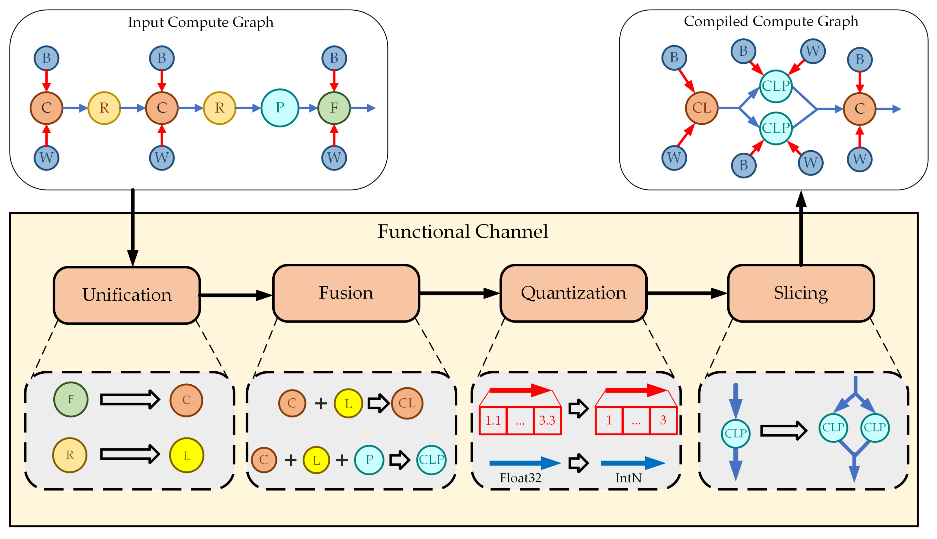
6.2. Functional Channel

The functional channel is a critical part of the compilation toolchain which is used to compile the compute graph. Compilation functions for CNN are implemented in the functional channel. The effects of all compilation functions are reflected in the compiled compute graph.

The functional channel consists of a series of independent sub-modules, and each sub-module implements one compilation function. Considering that the compilation toolchain bridges the CNN models and hardware accelerator, the sub-modules in the functional channel are responsible not only for implementing the proposed CNN optimization methods, but also for making sure the compute graph corresponds to the proposed hardware accelerator architecture. As shown in Figure 14, sub-modules of unification, fusion, quantization, and slicing are built in the functional channel.

After the compute graph is constructed, the functional channel takes the compute graph as input and processes it with all sub-modules. The unification module implements the compilation function by building new convolution nodes to replace FC nodes and building LeakyReLU nodes to replace Relu nodes. In addition, the operation attributes are generated by unification module and stored in the new nodes. The fusion module is used to fuse compute nodes. In the compute graph, the running tensor represents the access to the off-chip memory. However, our PE continuously processes convolution, BN, LeakyReLU, and pooling in the pipeline. Therefore, node fusion is adopted to remove redundant running tensors and ensure that the compute graph corresponds to the hardware architecture.

The quantization module implements compilation function by processing the tensors in the compute graph. Before the inference phase, running tensors are simply placeholders without data. Therefore, the quantization module only modifies the data type and data volume of running tensors. For para tensors, since the parameters of CNN are stored within it, the quantization module quantizes the parameters according to the quantization equation, thereby implementing the hybrid quantization method. The slicing module picks out layers in which the feature map slicing needs to be performed based on the dynamic slicing strategy. After the sliced layers are determined, the nodes and tensors of the sliced layers are copied and modified based on the number of sliced blocks, and the output tensors are concatenated to be the input of the next node.

6.3. Memory Allocator

In computer science, memory allocation is the process by which computer programs are assigned with memory space. A classical register allocation algorithm is the linear scan algorithm [67]. The linear scan algorithm uses live intervals to indicate the time ranges where the variables in the program are active. By comparing the overlap of the live intervals, the interfered variables are identified and appropriate memory space for each variable is allocated. In our memory allocator, we apply the linear scan algorithm to the compute graph and allocate the off-chip memory space for each tensor in CNN.

In the process of memory allocation, we traverse all tensors in the compute graph and calculate the size of memory space required by each tensor based on the dimension information. After that, the live interval list of compute graph is established and the overlaps between live intervals are analyzed. Tensors that interfere with each other cannot be allocated to the same space, and the space of non-interfered tensors can overlap to reduce the memory overhead. Notably, considering that the accelerator often needs to process multiple input images, parameter tensors are stored in off-chip memory fixedly until the deployed CNN is changed. In contrast, the spaces of the running tensors are released immediately after the computations in which the tensors participate are finished. Figure 15 shows the processing flow of the memory allocator. After memory allocation is completed, each tensor is filled with the information on its allocated address and size.

6.4. Instruction Generator

The instruction generator is responsible for converting the compiled compute graph into a parameter file and hardware instructions. Parameters are extracted from parameter tensors and organized into a parameter file which can be stored in off-chip memory directly. Hardware instructions are machine codes used to control the hardware accelerator. To meet the control requirements of the hardware accelerator, especially the PE configuration system, a hardware instruction set is designed to map the compute graph to the hardware accelerator.

The hardware instruction set is a set of binary codes with a length of 32 bits. The first eight bits of the 32-bit code are used as the identification header. Instructions can be divided into three categories, namely, configuration instructions, data movement instructions, and handshake instructions. Configuration instructions contain all information required by PE configuration units. The configuration information is decoded by hardware and converted into different control signals transferred to PE. The data movement instruction is responsible for the interaction with off-chip memory, including reading data from and writing data to the specific address. Notably, since the address and data length are often large numbers, the data movement instructions are designed as multi-level instructions, which means several instructions are combined to implement one function. Handshake instructions are used to indicate the start and end of a configuration process or a calculation stage. Examples of the three types of instructions are shown in Figure 16.

With the help of the customized hardware instruction set, the instruction generator implements the mapping from the compute graph to hardware. As shown in Figure 17, for each type of fused compute node, a corresponding pre-written instruction block is built. An instruction generator can traverse the compute graph and extract network information from the compute graph. After that, the instruction generator transfers the network information to the pre-written instruction blocks, and use the information to assign instructions. In this way, the conversion from the compute graph to hardware instructions is achieved. The instruction block starts and ends with a handshake instruction. In the instruction block, the configuration instructions are processed first, and then the data movement instructions are executed. Configuration instructions and data movement instructions are also separated by handshake instructions. In hardware, the configuration of the PE is completed first, and then the calculation process of the hardware accelerator is triggered by data movement instruction. After one cycle, the pipeline calculation of the accelerator is finished, and the data movement instructions write the resulting data back to the off-chip memory. Multiple instruction blocks are concatenated together to form an instruction file that can map the compiled CNN model to hardware.

7. Experiments and Performance Evaluation

In this section, network deployment experiments based on the proposed solution are introduced. Details of the experiments are illustrated, results of the experiments are demonstrated, and comparisons among different works are made to evaluate the performance of our work.

7.1. Experimental Settings

Experimental environments and methods are introduced in this subsection.

7.1.1. Experimental Methods and Dataset

To evaluate the effectiveness of the proposed deployment solution, a scene classification experiment based on the improved VGG16 network and an object detection experiment based on the improved YOLOv2 network were designed.

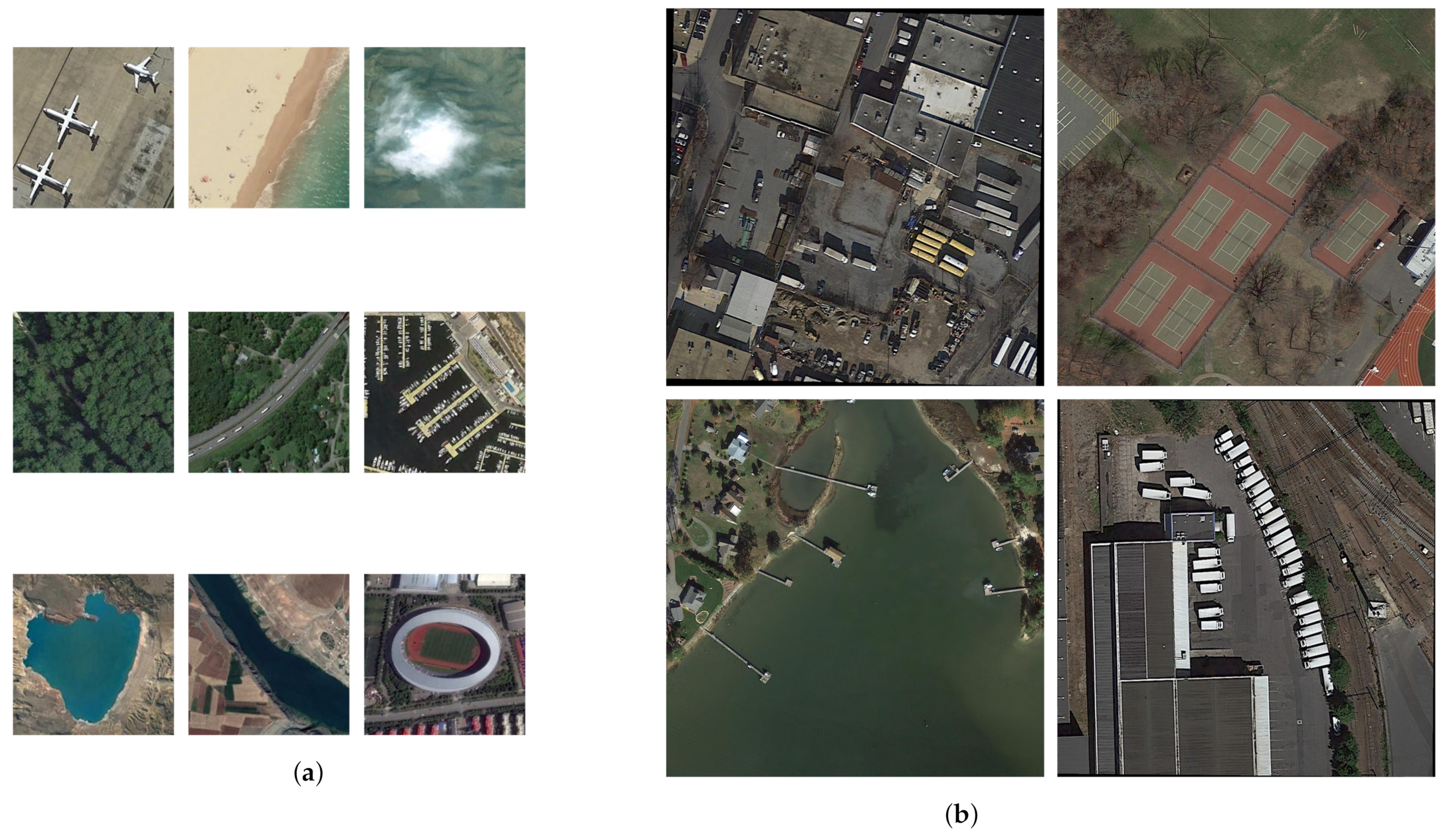
For scene classification, the NWPU-RESISC45 dataset [68] was used for evaluation. NWPU-RESISC45 contains 31,500 images and covers 45 scene classes with 700 images in each class, and the size of each image is fixed to 256 × 256. In our experiment, 20% images were used for training and 80% images were used for testing. Several sample images from the testing set of NWPU-RESISC45 are shown in Figure 18a.

For object detection, the large-scale DOTA-v1.0 dataset [69] was used for evaluation. This dataset contains 15 common categories, 2806 aerial images, and 188,282 instances; and the resolution range of images is from 800 × 800 to 6000 × 6000. The proportions of the training set, validation set, and testing set are 1/2, 1/6, and 1/3, respectively. The validation set is used for testing in our experiments. Notably, in the training process, all images are cropped to 1024 × 1024 patches by the DOTA development kit. Thus, in the testing process, all images are cropped to the same size with the stride of 512. Several sample images from the validation set of DOTA are shown in Figure 18b.

For scene classification, only one number is required to indicate the category of each image. Therefore, the classification overall accuracy (OA) can be directly calculated from the number of correct results n and the number of total test images N, as shown in Equation (20):

$$\mathrm{OA}=\frac{n}{N}\times 100\%.$$

(20)

For object detection, the detection results involve not only the category of targets, but also the position and size of the bounding boxes, which are more complicated to evaluate. We use a metric called mean average precision (mAP) to evaluate the detection performance. The mAP computes precision and recall to obtain average precision (AP) and counts the mean AP over all categories [70]. Therefore, it can reflect the overall detection accuracy.

7.1.2. Experimental Procedure

To evaluate the performance of the hardware accelerator, the proposed accelerator was implemented on a Xilinx AC701 evaluation board, which was equipped with an xc7a200t FPGA chip and a 1GB DDR3 SDRAM. DDR3 was used to store the images, parameters, and intermediate result of each layer during the inference phase. Eight parallel PEs were implemented to obtain a trade-off between resources and performance. A MicroBlaze (MB) soft processor core from Xilinx, San Jose, CA, USA was implemented on FPGA to control the hardware system. The project was built with VHDL. Vivado Design Suite 2019.2 from Xilinx, San Jose, CA, USA was used for synthesis and implementation.

To build the deployment system, a host PC was connected to the evaluation board. As shown in Figure 19, the host PC carried the images to be processed, the compilation toolchain, and the CNN models. After the compilation, the toolchain generated an instruction file and a parameter file for each CNN model. These two files and the images to be processed were transmitted to the evaluation board through 1000 M Ethernet.

A memory scheduling system was built on the evaluation board. A Memory Interface Generator (MIG) which supported the AXI4 interface was connected to DDR3 to provide a memory interface. An Ethernet Direct Memory Access (DMA) and PE DMA were implemented to interact with the MIG through the AXI4 bus system. After the Ethernet port of the evaluation board received the data the from host PC, parameters and images were transferred to DDR3 through Ethernet DMA, and the instruction file was directly handed to the processor core to be parsed. The processor core passed the configuration instructions to a decoder to perform PE configuration. Then, the calculation of PEs was initiated by handshake instructions and data movement instructions. Handshake instructions controlled the handshake between PE DMA and PEs, and data movement instructions implemented data transfer between DDR3 and PEs. Once the calculation of PEs was finished, the results were transmitted back to the host PC through the Ethernet to complete the detection or classification.

7.2. Experimental Result

Firstly, the resource utilization of the hardware implementation is analyzed, and the result is shown in

Table 1. Resource utilization of the hardware implementation.

Resource	LUT	FF	BRAM	DSP
Available	133,800	267,600	365	740
Utilization (full system)	49,817	59,622	129	94
Utilization (full system %)	37.23	22.28	35.34	12.70
Utilization (accelerator)	29,391	38,573	106	94
Utilization (accelerator %)	21.97	14.41	29.04	12.70

. We present the resource utilization of the full hardware system and the core accelerator. The full hardware system was the full implementation on FPGA, which not only contained the CNN accelerator but also contained the Microblaze, Ethernet port, Ethernet DMA, and MIG.

As shown in Table 1, for the full system, the utilization of LUT, Flip-Flop, BRAM, and DSP was 49,817, 59,622, 129, and 94, respectively. For the core accelerator, the utilization of LUT, Flip-Flop, BRAM, and DSP was 29,391, 38,573, 106, and 94, respectively. Most BRAMs are used for the construction of the input buffer and intermediate buffer. DSPs are consumed by the acceleration modules in PE. The available hardware resources of xc7a200t are strictly limited. Nonetheless, the resource utilization percent of the implemented hardware system is below 40%. This result demonstrated that our solution has great potential to adapt to spaceborne remote sensing platforms with extremely limited hardware resources.

Secondly, inference time, throughput, and power consumption of the hardware accelerator are evaluated. For throughput, the GOPs (giga operations) were used to measure how many operations a network had, and the GOPS (giga operations per second) was used as the criterion of throughput. We count that improved VGG16 had 40.96 GOPs, and improved YOLOv2 had 379.55 GOPs. For power consumption, the Xilinx power estimator was used to obtain the on-chip power information. The result shows that under 200 M clock frequency, the inference time for improved VGG16 was 1.78 s, and the inference time for improved YOLOv2 was 17.12 s. Therefore, for improved VGG16 and improved YOLOv2, the throughput of the accelerator was 23.06 or 22.17 GOPS, respectively. Relatively, the total on-chip power of the hardware accelerator was 3.407 W, and the power consumption of the core PEs was only 0.919 W. Therefore, the throughput per watt of the accelerator was 6.77 GOPS for improved VGG16 and and 6.51 GOPS for improved YOLOv2. Additionally, the throughput per watt of the core PEs reached 25.09 GOPS for improved VGG16 and 24.12 GOPS for improved YOLOv2. The results show that the proposed hardware accelerator is suitable for spaceborne scenarios where the power consumption is limited. In addition, the energy cost per inference of the accelerator was 6.1 for improved VGG16 and and 58.1 J for improved YOLOv2. The energy cost per inference of the core PEs was 1.6 for improved VGG16 and 15.7 J for improved YOLOv2.

Thirdly, we evaluate the experimental results of scene classification and object detection. The improved VGG16 network was deployed with our solution successfully, the model size was reduced from 59.0 to 14.8 MB after compilation, and the time spent on compilation was only 0.36 s. The classification was processed on the NWPU-RESISC45 testing set, and an overall accuracy of 88.08% was obtained. Some results of classification are shown in Figure 20a. The improved YOLOv2 network was deployed with our solution successfully, the model size was reduced from 197.5 to 49.4 MB after compilation, and the time spent on compilation was only 1.08 s. The detection was performed on the DOTA validation set, and the mAP reached 67.30%. Some detection results are shown in Figure 20b.

On the one hand, the experimental results show that our solution achieves network model compilation, and the very small compilation time consumption proves that our solution can perform real-time mapping of network models to hardware accelerators. On the other hand, the experimental results show that our solution achieves high accuracy when performing remote-sensing scene classification tasks and remote-sensing object detection tasks.

7.3. Performance Comparison

To show the effectiveness of the proposed deployment solution, a series of comparative experiments were conducted. Firstly, we implemented the remote-sensing scene classification algorithm and remote-sensing object detection algorithm on central processing unit (CPU) and graphic processing unit (GPU) platforms. The networks used by the algorithms were exactly the same as the networks run on the proposed hardware accelerator; thus, the performances on the CPU, GPU, and the proposed hardware accelerator can be compared. The used CPU was Intel Xeon Gold 5120T with 128 GB DDR4 DRAM, and the used GPU was NVIDIA Titan Xp with 12 GB GDDR5X memory.

Table 2. Evaluation results on the central processing unit (CPU), graphic processing unit (GPU), and proposed accelerator.

	CPU		GPU		FPGA
Device	Intel Xeon Gold 5120T		Nvidia Titan Xp		Xilinx AC701
Technology (nm)	14		16		28
Frequency (MHz)	2200		1582		200
Power(w)	105		250		3.407
Network	Improved VGG16	Improved YOLOv2	Improved VGG16	Improved YOLOv2	Improved VGG16	Improved YOLOv2
Accuracy (OA|mAP)	88.13	67.50	88.13	67.50	88.08	67.30
Throughput (GOPS)	208.8	58.9	5543.4	5279.4	23.06	22.17
Power Efficiency (GOPS/W)	1.99	0.56	22.17	21.12	6.77 (25.09) 1	6.51 (24.12) 1

¹ The numbers in () represent the results of the core PEs.

shows the performance comparison among the CPU, GPU, and proposed accelerator.

As shown in Table 2, the thermal design powers of the CPU and GPU are 105 and 250 W, which are 31× and 73× higher than the 3.407 W power consumption of the proposed hardware accelerator, respectively. Obviously, our accelerator is more suitable for power-limited spaceborne remote sensing applications. The throughputs of the CPU and GPU were better than that of the proposed accelerator, regardless of which network was deployed. However, the CPU was at a disadvantage when comparing power efficiency. For the improved VGG16 network, the power efficiency of CPU was only 1.99 GOPS/W, and the power efficiency of our accelerator was 6.77 GOPS/W. For the improved YOLOv2 network, the power efficiency of CPU was only 0.56 GOPS/W, and the power efficiency of our accelerator was 6.51 GOPS/W. Compared to CPU, the proposed hardware accelerator achieved about 3.4–11.6× better power efficiency. The power efficiency of GPU was greater the power efficiency of our accelerator. However, the main frequency of the GPU was 8× higher than the main frequency of our FPGA-based accelerator, and the power efficiency of the GPU was only about 3× better than that of our accelerator.

Additionally, as mentioned in the previous subsection, the core PEs achieved 25.09 GOPS/W power efficiency for the improved VGG16 network and 24.12 GOPS/W power efficiency for the improved YOLOv2 network, both of which are better than the power efficiency of the GPU. In hardware implementation, we only implemented eight parallel PEs for evaluation. Therefore, the power efficiency of our accelerator can be improved by increasing the number of PEs, which is easy to implement in hardware. Furthermore, we can reduce the power consumption and resource consumption by reducing the number of PEs. Although system performance will be degraded, the accelerator can thus adapt to the extremely resource-limited spaceborne scenario. Hardware accelerators with dynamic adjustment characteristics can play an important role in spaceborne remote sensing applications.

Table 2 also shows the comparison of classification and detection accuracy between different platforms. For scene classification tasks, the OA result obtained from our hardware dropped by only 0.05% compared to the results from the CPU and GPU. For object detection tasks, the mAP result obtained from our hardware dropped by only 0.2% compared to the results from the CPU and GPU. The reason for the loss of accuracy is considered to be the limitation in floating-point precision. When the compilation toolchain performs quantization calculations, the number of significant figures for floating-point data is limited to six, which results in slight errors. This accuracy loss is acceptable in practical applications.

Table 3. Performance comparison of our work with previous accelerators.

	[71]	[72]	[73]	Our Work	[74]	[75]	[76]	Our Work
Platform	Intel Stratix 10 GX 2800	Xilinx Zynq xc7z045	Xilinx Zynq xc7z045	Xilinx AC701	Xilinx PYNQ	Xilinx ZCU102	Xilinx Zynq xc7z020	Xilinx AC701
Technology (nm)	14	28	28	28	28	16	28	28
Frequency (MHz)	300	150	100	200	100	300	150	200
Network	VGG16	VGG16	VGG16	Improved VGG16	YOLOv2	YOLOv2	YOLOv2	Improved YOLOv2
Quantization	8/16-bit	16-bit	16-bit	8-bit	16-bit	16-bit	16-bit	8-bit
LUTs	469,000 1	182,616	–	49,817 (29,391) 3	37,230	95,136	35,948	49,817 (29,391) 3
BRAMs	1345 2	486	–	129 (106) 3	87.5	246	87.5	129 (106) 3
DSPs	8216	780	64	94 (94) 3	151	609	149	94 (94) 3
Power (W)	100	9.63	–	3.407	2.32	11.8	2.39	3.407
Throughput (GOPS)	1604.57	137	12.5	23.06	14.10	102	26.23	22.17
Power Efficiency (GOPS/W)	16.05	14.2	–	6.77	6.08	8.64	10.97	6.51
DSP Efficiency (GOPS/DSP)	0.20	0.18	0.19	0.25	0.09	0.17	0.18	0.24

¹ For Intel FPGA, the logic unit refers to ALM. ² For Intel FPGA, the size of BRAM refers to 20 kb. We converted it into 36 kb for comparison. ³ The numbers in () represent the resources utilization of core accelerator only.

shows the performance comparison between the proposed deployment solution and previous works [71,72,73,74,75,76]. It should be noted that in Table 3, the resource utilization of our full hardware system and the resource utilization of our core accelerator are both listed. Our hardware platform AC701 is a pure FPGA platform, and the platforms in [72,73,74,75,76] all adopt ZYNQ System on Chip (SoC) architecture equipped with an ARM processor. Therefore, it is fairer to use the resource utilization of core accelerator as the reference value of our work in performance comparison. Compared to the works in [72,73,74,75,76], our hardware system spends additional resources on the parts of Microblaze softcore, Ethernet DMA, Ethernet port, and MIG. Table 3 shows that the resource consumption of our core accelerator is almost the least among all works, which indicates that our work has great potential to be applied on resource-limited spaceborne platforms.

The works introduced in references [71,72,73] are capable of accelerating the VGG16 network. Ma et al. [71] designed a hardware accelerator based on a large multiply–accumulate array structure and proposed an RTL-level compiler to map the network. Table 3 shows that the accelerator in [71] achieved a TOPS-level throughput. However, the cost of such excellent performance is the high consumption of hardware resources. Moreover, the power consumption of the accelerator in [71] reached 100W, which is unacceptable in power-limited scenarios. Guo et al. [72] proposed a CNN deployment scheme, including a model compiler and a hardware architecture with data control flow. Their hardware achieved good power efficiency. However, the hardware implementation in [72] consumes 780 DSPs, which is 8.3× more than the DSP consumption of our accelerator. In a resource-limited scenario, the architecture in [72] is difficult to implement. Chen et al. [73] proposed a CNN accelerator based on a channel-oriented convolutional computation strategy, which enables the accelerator to adapt to convolution kernels of different sizes. The DSP consumption in [73] was the smallest among all works. However, the throughput of the accelerator in [73] is only 12.5 GOPS.

The designs in [74,75,76] aim to accelerate YOLOv2 networks for object detection. Peng et al. [74] built a low-power YOLOv2 accelerator based on the PYNQ platform. The power consumption of the accelerator in [74] is 2.32 W, which is the lowest among all works. However, this accelerator only achieves 14.10 GOPS throughput. Zhang et al. [75] proposed a scheme to deploy the YOLOv2 network on the ZCU102 platform. The accelerator in [75] achieves the great throughput of 102 GOPS. However, its power consumption reaches 11.8 W, which limits its application in power-sensitive scenarios. Xiao et al. [76] successfully deployed the YOLOv2 network on the xc7z020 FPGA through a series of optimization methods. The resource consumption of the hardware in [76] is kept at a low level, and the power consumption of the hardware in [76] is only 2.39 W. However, DSP consumption of the hardware in [76] was 1.59× more than that of our hardware system.

For FPGA-based designs, the resource consumption varies in different architectures. The outstanding throughput performance of a hardware implementation may be mainly due to the massive usage of hardware resources. DSP is the core resource for building a processing engine array in a CNN accelerator; the utilization of DSP greatly determines the scale of the processing engine. Therefore, in order to compare the performances of different architectures fairly, we used DSP efficiency as the indicator. DSP efficiency is defined as the number of GOPS that each DSP can perform throughout the entire processing of the hardware. The usage of DSP efficiency can exclude the effect of differences in hardware resources usage and help to compare performances among accelerators of different scales. As shown in Table 3, the DSP efficiency of our hardware reached 0.25 GOPS/DSP and 0.24 GOPS/DSP for the improved VGG16 network and the improved YOLOv2 network, respectively. Both values are the highest in the comparison with previous works, which indicates that with the same scale processing engine, our accelerator would have better throughput performance. The comparison with previous works on various indicators illustrated that our accelerator achieved a great trade-off between power consumption, resource consumption, and throughput.

8. Conclusions

This paper proposed an automatic CNN deployment solution for spaceborne remote sensing applications, including algorithm optimization methods, a hardware acceleration architecture, and a compilation toolchain. Firstly, a series of CNN optimization methods, including operation unification and integration, convolution dataflow rearrangement, and dynamic slicing strategy, are used to decrease the CNN scale and simplify the CNN computation. Secondly, we proposed an efficient hardware architecture for CNN acceleration. A weight-reused convolutional computation module was illustrated, and a reconfigurable and scalable PE array was built to process diverse CNNs. Finally, a compilation toolchain was designed to automatically convert the CNN models into hardware instructions. Real-time mapping from the optimized CNN algorithms to the proposed hardware accelerator was achieved. With the proposed CNN deployment solution, the improved VGG16 and improved YOLOv2 were successfully deployed on Xilinx AC701 with low accuracy loss. The experimental results show that the power consumption of the proposed solution was only 3.407 W, and the DSP resource consumption of the proposed solution was only 94. For the classification task, the throughput of the proposed solution was 23.06 GOPS, and the DSP efficiency of the proposed solution was 0.25 GOPS/DSP. For the detection task, the throughput of the proposed solution was 22.17 GOPS, and the DSP efficiency of the proposed solution was 0.24 GOPS/DSP. The results show that the proposed CNN deployment solution features low power consumption, low resources consumption, and real-time mapping of various networks. With these features, our solution has great potential for CNN-based spaceborne remote sensing image processing.

In future, we plan to optimize the pipeline stages of the accelerator and implement the optimized accelerator on radiation-hardened FPGA to evaluate the robustness and effectiveness of the proposed solution. Furthermore, we plan to build an ASIC-based solution to explore extreme resource efficiency for spaceborne remote sensing applications.