
Comparison of Deep Learning Methods for Detecting and Counting Sorghum Heads in UAV Imagery


Abstract
:
1. Introduction
2. Materials and Methods
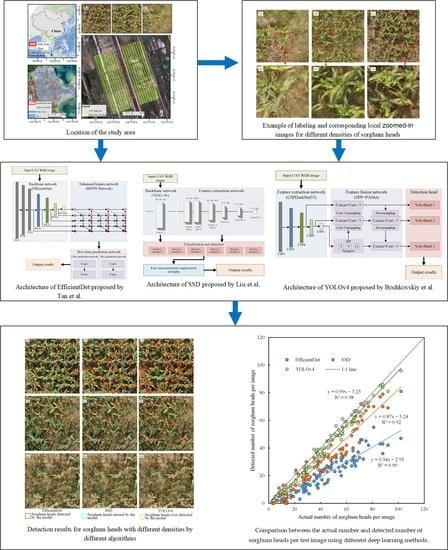
2.1. Study Area
2.2. Data Collection and Preparation
2.2.1. UAV Image Collection
2.2.2. UAV Image Dataset Construction
2.2.3. Image Labeling
3. Method
3.1. Deep Learning Algorithms
3.1.1. EfficientDet
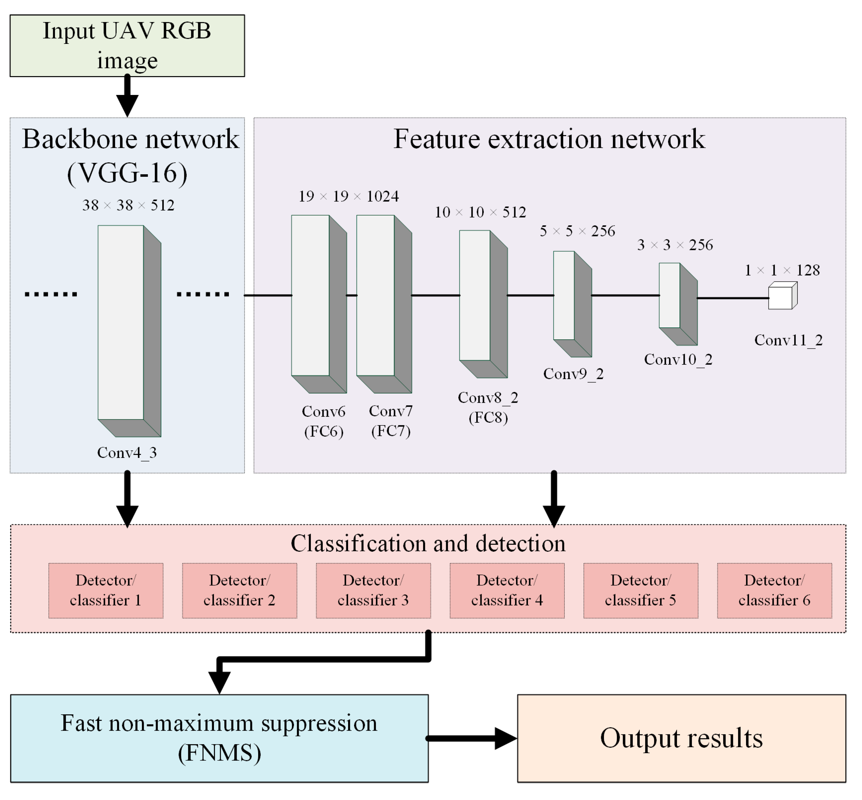
3.1.2. SSD
3.1.3. YOLOv4
3.2. Programming and Model Training Environment
3.2.1. Programming Environment
3.2.2. Transfer Learning and Training
3.3. Designing the Experiments
3.4. Evaluation Metrics
4. Results
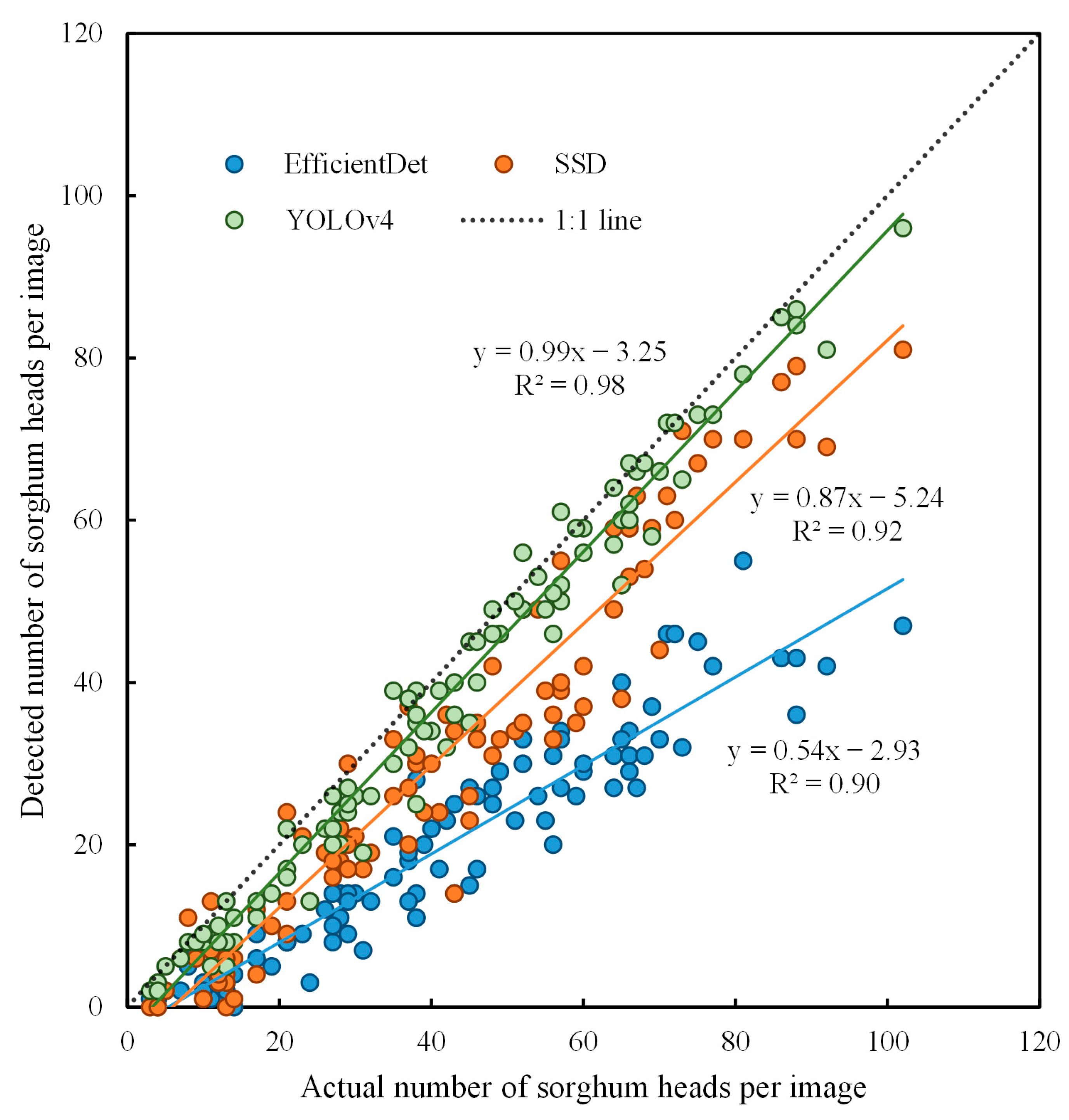
4.1. Comparison of the Detection Results with Different Model Algorithms
4.2. Performance Evaluation of Different Models for Sorghum Head Detection
4.2.1. Evaluation of Positive and Negative Samples for Different Models
4.2.2. Accuracy Evaluation of Different Methods
4.2.3. Comparison of Computational Efficiency of Different Methods
4.3. Comparison of Overlap Ratio Thresholds
4.4. Comparison of Confidence Values
4.5. Comparison of IoU Thresholds
5. Discussion
5.1. Effect of Different DL Methods on Sorghum Head Detection
5.2. Effect of Model Parameters on Sorghum Head Detection
5.3. Effects of Other Factors
6. Conclusions
- (1)
- Among the three DL methods, YOLOv4 had the highest accuracy in sorghum head detection, with a detection rate of positive samples at 94.12%, P of 97.62%, R of 64.20%, and AP and F1 scores of 84.51% and 0.77, respectively. Although the average elapsed time of the training epoch was 32 s, which was not as efficient as EfficientDet and SSD, the image detection time was 0.0451, which was more efficient than EfficientDet.
- (2)
- For the analysis of the model parameters, it was concluded that the highest sorghum head detection accuracy was obtained when the overlap ratios, confidence, and IoU were each 0.3.
Author Contributions
Funding
Acknowledgments
Conflicts of Interest
References
- Lipper, L.; Thornton, P.; Campbell, B.M.; Baedeker, T.; Braimoh, A.; Bwalya, M.; Caron, P.; Cattaneo, A.; Garrity, D.; Henry, K. Climate-smart agriculture for food security. Nat. Clim. Chang. 2014, 4, 1068–1072. [Google Scholar] [CrossRef]
- Li, H.; Chen, Z.; Liu, G.; Jiang, Z.; Huang, C. Improving Winter Wheat Yield Estimation from the CERES-Wheat Model to Assimilate Leaf Area Index with Different Assimilation Methods and Spatio-Temporal Scales. Remote Sens. 2017, 9, 190. [Google Scholar] [CrossRef] [Green Version]
- Xu, X.; Li, H.; Yin, F.; Xi, L.; Qiao, H.; Ma, Z.; Shen, S.; Jiang, B.; Ma, X. Wheat ear counting using K-means clustering segmentation and convolutional neural network. Plant Methods 2020, 16, 106. [Google Scholar] [CrossRef] [PubMed]
- Ma, J.; Li, Y.; Liu, H.; Wu, Y.; Zhang, L. Towards improved accuracy of UAV-based wheat ears counting: A transfer learning method of the ground-based fully convolutional network. Expert Syst. Appl. 2022, 191, 116226. [Google Scholar] [CrossRef]
- Zhao, Y.; Zheng, B.; Chapman, S.C.; Laws, K.; George-Jaeggli, B.; Hammer, G.L.; Jordan, D.R.; Potgieter, A.B. Detecting Sorghum Plant and Head Features from Multispectral UAV Imagery. Plant Phenomics 2021, 2021, 9874650. [Google Scholar] [CrossRef]
- Lin, Z.; Guo, W. Sorghum Panicle Detection and Counting Using Unmanned Aerial System Images and Deep Learning. Front. Plant Sci. 2020, 11, 534853. [Google Scholar] [CrossRef]
- Wu, J.; Yang, G.; Yang, X.; Xu, B.; Han, L.; Zhu, Y. Automatic Counting of in situ Rice Seedlings from UAV Images Based on a Deep Fully Convolutional Neural Network. Remote Sens. 2019, 11, 691. [Google Scholar] [CrossRef] [Green Version]
- Osco, L.P.; dos Santos de Arruda, M.; Gonçalves, D.N.; Dias, A.; Batistoti, J.; de Souza, M.; Gomes, F.D.G.; Ramos, A.P.M.; de Castro Jorge, L.A.; Liesenberg, V.; et al. A CNN approach to simultaneously count plants and detect plantation-rows from UAV imagery. ISPRS J. Photogramm. Remote Sens. 2021, 174, 1–17. [Google Scholar] [CrossRef]
- Lu, H.; Liu, L.; Li, Y.; Zhao, X.; Wang, X.; Cao, Z. TasselNetV3: Explainable Plant Counting with Guided Upsampling and Background Suppression. IEEE Trans. Geosci. Remote Sens. 2022, 60, 4700515. [Google Scholar] [CrossRef]
- Wei, L.; Luo, Y.; Xu, L.; Zhang, Q.; Cai, Q.; Shen, M. Deep Convolutional Neural Network for Rice Density Prescription Map at Ripening Stage Using Unmanned Aerial Vehicle-Based Remotely Sensed Images. Remote Sens. 2022, 14, 46. [Google Scholar] [CrossRef]
- Ampatzidis, Y.; Partel, V.; Costa, L. Agroview: Cloud-based application to process, analyze and visualize UAV-collected data for precision agriculture applications utilizing artificial intelligence. Comput. Electron. Agric. 2020, 174, 105457. [Google Scholar] [CrossRef]
- Gnädinger, F.; Schmidhalter, U. Digital Counts of Maize Plants by Unmanned Aerial Vehicles (UAVs). Remote Sens. 2017, 9, 544. [Google Scholar] [CrossRef] [Green Version]
- Torres-Sánchez, J.; López-Granados, F.; Peña, J.M. An automatic object-based method for optimal thresholding in UAV images: Application for vegetation detection in herbaceous crops. Comput. Electron. Agric. 2015, 114, 43–52. [Google Scholar] [CrossRef]
- García-Martínez, H.; Flores-Magdaleno, H.; Khalil-Gardezi, A.; Ascencio-Hernández, R.; Tijerina-Chávez, L.; Vázquez-Peña, M.A.; Mancilla-Villa, O.R. Digital Count of Corn Plants Using Images Taken by Unmanned Aerial Vehicles and Cross Correlation of Templates. Agronomy 2020, 10, 469. [Google Scholar] [CrossRef] [Green Version]
- Barreto, A.; Lottes, P.; Ispizua Yamati, F.R.; Baumgarten, S.; Wolf, N.A.; Stachniss, C.; Mahlein, A.; Paulus, S. Automatic UAV-based counting of seedlings in sugar-beet field and extension to maize and strawberry. Comput. Electron. Agric. 2021, 191, 106493. [Google Scholar] [CrossRef]
- Vong, C.N.; Conway, L.S.; Zhou, J.; Kitchen, N.R.; Sudduth, K.A. Early corn stand count of different cropping systems using UAV-imagery and deep learning. Comput. Electron. Agric. 2021, 186, 106214. [Google Scholar] [CrossRef]
- Feng, A.; Zhou, J.; Vories, E.; Sudduth, K.A. Evaluation of Cotton Emergence Using UAV-Based Narrow-Band Spectral Imagery with Customized Image Alignment and Stitching Algorithms. Remote Sens. 2020, 12, 1764. [Google Scholar] [CrossRef]
- Madec, S.; Jin, X.; Lu, H.; de Solan, B.; Liu, S.; Duyme, F.; Heritier, E.; Baret, F. Ear density estimation from high resolution RGB imagery using deep learning technique. Agric. For. Meteorol. 2019, 264, 225–234. [Google Scholar] [CrossRef]
- Wang, L.; Xiang, L.; Tang, L.; Jiang, H. A Convolutional Neural Network-Based Method for Corn Stand Counting in the Field. Sensors 2021, 21, 507. [Google Scholar] [CrossRef]
- Liu, Y.; Cen, C.; Che, Y.; Ke, R.; Ma, Y.; Ma, Y. Detection of Maize Tassels from UAV RGB Imagery with Faster R-CNN. Remote Sens. 2020, 12, 338. [Google Scholar] [CrossRef] [Green Version]
- Ghosal, S.; Zheng, B.; Chapman, S.C.; Potgieter, A.B.; Jordan, D.R.; Wang, X.; Singh, A.K.; Singh, A.; Hirafuji, M.; Ninomiya, S.; et al. A Weakly Supervised Deep Learning Framework for Sorghum Head Detection and Counting. Plant Phenomics 2019, 2019, 1525874. [Google Scholar] [CrossRef] [PubMed] [Green Version]
- Guo, W.; Zheng, B.; Potgieter, A.B.; Diot, J.; Watanabe, K.; Noshita, K.; Jordan, D.R.; Wang, X.; Watson, J.; Ninomiya, S.; et al. Aerial Imagery Analysis—Quantifying Appearance and Number of Sorghum Heads for Applications in Breeding and Agronomy. Front. Plant Sci. 2018, 9, 1544. [Google Scholar] [CrossRef] [PubMed] [Green Version]
- Kamilaris, A.; Prenafeta-Boldú, F.X. Deep learning in agriculture: A survey. Comput. Electron. Agric. 2018, 147, 70–90. [Google Scholar] [CrossRef] [Green Version]
- Chapelle, O.; Vapnik, V.; Bousquet, O.; Mukherjee, S. Choosing multiple parameters for support vector machines. Mach. Learn. 2002, 46, 131–159. [Google Scholar] [CrossRef]
- Breiman, L. Random Forests. Mach. Learn. 2001, 5, 5–32. [Google Scholar] [CrossRef] [Green Version]
- Bengio, Y.; Courville, A.; Vincent, P. Representation Learning: A Review and New Perspectives. IEEE Trans. Pattern Anal. Mach. Intell. 2013, 35, 1798–1828. [Google Scholar] [CrossRef] [PubMed]
- LeCun, Y.; Bengio, Y.; Hinton, G. Deep learning. Nature 2015, 521, 436–444. [Google Scholar] [CrossRef] [PubMed]
- Ba, L.J.; Caruana, R. Do Deep Nets Really Need to be Deep? In Proceedings of the Advances in Neural Information Processing Systems 27 (NIPS 2014), Montreal, QC, Canada, 8–13 December 2014; MIT Press: Cambridge, MA, USA, 2014; pp. 2654–2662. [Google Scholar]
- Shelhamer, E.; Long, J.; Darrell, T. Fully Convolutional Networks for Semantic Segmentation. EEE Trans. Pattern Anal. Mach. Intell. 2017, 39, 640–651. [Google Scholar] [CrossRef]
- Ronneberger, O.; Fischer, P.; Brox, T. U-Net: Convolutional Networks for Biomedical Image Segmentation. In Proceedings of the Medical Image Computing and Computer-Assisted Intervention, Munich, Germany, 5–9 October 2015; Springer: Cham, Switzerland, 2015; Volume 9351, pp. 234–241. [Google Scholar]
- Sadeghi-Tehran, P.; Virlet, N.; Ampe, E.M.; Reyns, P.; Hawkesford, M.J. DeepCount: In-Field Automatic Quantification of Wheat Spikes Using Simple Linear Iterative Clustering and Deep Convolutional Neural Networks. Front. Plant Sci. 2019, 10, 1176. [Google Scholar] [CrossRef]
- Zhang, Y.; Zhou, D.; Chen, S.; Gao, S.; Ma, Y. Single-Image Crowd Counting via Multi-Column Convolutional Neural Network. In Proceedings of the 2016 IEEE Conference on Computer Vision and Pattern Recognition (CVPR), Las Vegas, NV, USA, 27–30 June 2016; pp. 589–597. [Google Scholar]
- Li, Y.; Zhang, X.; Chen, D. CSRNet: Dilated Convolutional Neural Networks for Understanding the Highly Congested Scenes. In Proceedings of the 31st IEEE/CVF Conference on Computer Vision and Pattern Recognition (CVPR), Salt Lake City, UT, USA, 18–23 June 2018; pp. 1091–1100. [Google Scholar]
- Ren, S.; He, K.; Girshick, R.; Sun, J. Faster R-CNN: Towards Real-Time Object Detection with Region Proposal Networks. IEEE Trans. Pattern Anal. Mach. Intell. 2017, 39, 1137–1149. [Google Scholar] [CrossRef] [Green Version]
- Tan, M.; Pang, R.; Le, Q.V. EfficientDet: Scalable and Efficient Object Detection. In Proceedings of the 2020 IEEE/CVF Conference on Computer Vision and Pattern Recognition (CVPR), Seattle, WA, USA, 13–19 June 2020; pp. 10778–10787. [Google Scholar]
- Liu, W.; Anguelov, D.; Erhan, D.; Szegedy, C.; Reed, S.; Fu, C.; Berg, A.C. SSD: Single shot multibox detector. In Proceedings of the 14th European Conference on Computer Vision (ECCV), Amsterdam, The Netherlands, 11–14 October 2016. [Google Scholar]
- Redmon, J.; Divvala, S.; Girshick, R.; Farhadi, A. You Only Look Once: Unified, Real-Time Object Detection. In Proceedings of the 2016 IEEE Conference on Computer Vision and Pattern Recognition (CVPR), Las Vegas, NV, USA, 27–30 June 2016; pp. 779–788. [Google Scholar]
- FAO. Statistical Database of the Food and Agricultural Organization of the United Nations. 2017. Available online: https://www.fao.org/faostat/en/#data (accessed on 30 May 2022).
- Li, H.; Huang, C.; Liu, Q.; Liu, G. Accretion–Erosion Dynamics of the Yellow River Delta and the Relationships with Runoff and Sediment from 1976 to 2018. Water 2020, 12, 2992. [Google Scholar] [CrossRef]
- Li, H.; Chen, Z.; Jiang, Z.; Sun, L.; Liu, K.; Liu, B. Temporal-spatial variation of evapotranspiration in the Yellow River Delta based on an integrated remote sensing model. J. Appl. Remote Sens. 2015, 9, 96047. [Google Scholar] [CrossRef]
- LabelImg. 2022. Available online: https://github.com/tzutalin/labelImg (accessed on 30 May 2022).
- Lin, T.; Maire, M.; Belongie, S.; Hays, J.; Perona, P.; Ramanan, D.; Ar, P.D.; Zitnick, C.L. Microsoft COCO: Common Objects in Context. In Proceedings of the 13th European Conference on Computer Vision (ECCV), Zurich, Switzerland, 6–12 September 2014. [Google Scholar]
- Tan, M.; Le, Q.V. EfficientNet: Rethinking Model Scaling for Convolutional Neural Networks. In Proceedings of the International Conference on Machine Learning 2019, Long Beach, CA, USA, 9–15 June 2019. [Google Scholar]
- Simonyan, K.; Zisserman, A. Very Deep Convolutional Networks for Large-Scale Image Recognition. In Proceedings of the 3rd International Conference on Learning Representations, ICLR 2015, San Diego, CA, USA, 7–9 May 2015. [Google Scholar]
- Li, X.; Liu, C.; Dai, S.; Lian, H.; Ding, G. Scale specified single shot multibox detector. IET Comput. Vis. 2020, 14, 59–64. [Google Scholar] [CrossRef]
- Yi, J.; Wu, P.; Metaxas, D.N. ASSD: Attentive single shot multibox detector. Comput. Vis. Image Underst. 2019, 189, 102827. [Google Scholar] [CrossRef] [Green Version]
- Bochkovskiy, A.; Wang, C.; Liao, H.M. YOLOv4: Optimal Speed and Accuracy of Object Detection. arXiv 2020, arXiv:2004.10934. [Google Scholar]
- Redmon, J.; Farhadi, A. YOLOv3: An Incremental Improvement. arXiv 2018, arXiv:1804.02767. [Google Scholar]
- Tian, Y.; Yang, G.; Wang, Z.; Wang, H.; Li, E.; Liang, Z. Apple detection during different growth stages in orchards using the improved YOLO-V3 model. Comput. Electron. Agric. 2019, 157, 417–426. [Google Scholar] [CrossRef]
- Zakria, Z.; Deng, J.; Kumar, R.; Khokhar, M.S.; Cai, J.; Kumar, J. Multiscale and Direction Target Detecting in Remote Sensing Images via Modified YOLO-v4. IEEE J. Sel. Top. Appl. Earth Obs. Remote Sens. 2022, 15, 1039–1048. [Google Scholar] [CrossRef]
- Wu, D.; Lv, S.; Jiang, M.; Song, H. Using channel pruning-based YOLO v4 deep learning algorithm for the real-time and accurate detection of apple flowers in natural environments. Comput. Electron. Agric. 2020, 178, 105742. [Google Scholar] [CrossRef]
- Jiang, J.; Fu, X.; Qin, R.; Wang, X.; Ma, Z. High-Speed Lightweight Ship Detection Algorithm Based on YOLO-V4 for Three-Channels RGB SAR Image. Remote Sens. 2021, 13, 1909. [Google Scholar] [CrossRef]
- Shi, P.; Jiang, Q.; Shi, C.; Xi, J.; Tao, G.; Zhang, S.; Zhang, Z.; Liu, B.; Gao, X.; Wu, Q. Oil Well Detection via Large-Scale and High-Resolution Remote Sensing Images Based on Improved YOLO v4. Remote Sens. 2021, 13, 3243. [Google Scholar] [CrossRef]
- Zhuang, F.; Qi, Z.; Duan, K.; Xi, D.; Zhu, Y.; Zhu, H.; Xiong, H.; He, Q. A Comprehensive Survey on Transfer Learning. Proc. IEEE 2021, 109, 43–76. [Google Scholar] [CrossRef]
- Yosinski, J.; Clune, J.; Bengio, Y.; Lipson, H. How transferable are features in deep neural networks? In Proceedings of the 28th Conference on Neural Information Processing Systems (NIPS), Montreal, QC, Canada, 8–13 December 2014. [Google Scholar]
- Mekhalfi, M.L.; Nicolo, C.; Bazi, Y.; Rahhal, M.M.A.; Alsharif, N.A.; Maghayreh, E.A. Contrasting YOLOv5, Transformer, and EfficientDet Detectors for Crop Circle Detection in Desert. IEEE Geosci. Remote Sens. Lett. 2022, 19, 3003205. [Google Scholar] [CrossRef]
- Qin, P.; Cai, Y.; Liu, J.; Fan, P.; Sun, M. Multilayer Feature Extraction Network for Military Ship Detection from High-Resolution Optical Remote Sensing Images. EEE J. Sel. Top. Appl. Earth Obs. Remote Sens. 2021, 14, 11058–11069. [Google Scholar] [CrossRef]
- Kim, J.; Park, I.; Kim, S. A Fusion Framework for Multi-Spectral Pedestrian Detection using EfficientDet. In Proceedings of the 2021 21st International Conference on Control, Automation and Systems (ICCAS), Jeju, Korea, 12–15 October 2021; pp. 1111–1113. [Google Scholar]
- Majchrowska, S.; Mikołajczyk, A.; Ferlin, M.; Klawikowska, Z.; Plantykow, M.A.; Kwasigroch, A.; Majek, K. Deep learning-based waste detection in natural and urban environments. Waste Manag. 2022, 138, 274–284. [Google Scholar] [CrossRef] [PubMed]
- Ammar, A.; Koubaa, A.; Benjdira, B. Deep-Learning-Based Automated Palm Tree Counting and Geolocation in Large Farms from Aerial Geotagged Images. Agronomy 2021, 11, 1458. [Google Scholar] [CrossRef]
- Jia, S.; Diao, C.; Zhang, G.; Dun, A.; Sun, Y.; Li, X.; Zhang, X. Object Detection Based on the Improved Single Shot MultiBox Detector. In Proceedings of the International Symposium on Power Electronics and Control Engineering (ISPECE), Xi’an, China, 28–30 December 2018. [Google Scholar]
- Aziz, L.; Haji Salam, M.S.B.; Sheikh, U.U.; Ayub, S. Exploring Deep Learning-Based Architecture, Strategies, Applications and Current Trends in Generic Object Detection: A Comprehensive Review. IEEE Access 2020, 8, 170461–170495. [Google Scholar] [CrossRef]
- Zhang, C.; Li, T.; Zhang, W. The Detection of Impurity Content in Machine-Picked Seed Cotton Based on Image Processing and Improved YOLO V4. Agronomy 2022, 12, 66. [Google Scholar] [CrossRef]
- Gai, R.; Chen, N.; Yuan, H. A detection algorithm for cherry fruits based on the improved YOLO-v4 model. Neural Comput. Appl. 2021. [Google Scholar] [CrossRef]
- Li, M.; Zhang, Z.; Lei, L.; Wang, X.; Guo, X. Agricultural Greenhouses Detection in High-Resolution Satellite Images Based on Convolutional Neural Networks: Comparison of Faster R-CNN, YOLO v3 and SSD. Sensors 2020, 20, 4938. [Google Scholar] [CrossRef]
- Uzal, L.C.; Grinblat, G.L.; Namías, R.; Larese, M.G.; Bianchi, J.S.; Morandi, E.N.; Granitto, P.M. Seed-per-pod estimation for plant breeding using deep learning. Comput. Electron. Agric. 2018, 150, 196–204. [Google Scholar] [CrossRef]
- SC Chapman, M.; Olsen, P.; Ramamurthy, K.N. Counting and Segmenting Sorghum Heads. In Proceedings of the 2019 IEEE/CVF Conference on Computer Vision and Pattern Recognition Workshops (CVPRW), Long Beach, CA, USA, 16–17 June 2019. [Google Scholar]
- Chandra, A.L.; Desai, S.V.; Balasubramanian, V.N.; Ninomiya, S.; Guo, W. Active learning with point supervision for cost-effective panicle detection in cereal crops. Plant Methods 2020, 16, 34. [Google Scholar] [CrossRef] [PubMed]
- Velumani, K.; Lopez-Lozano, R.; Madec, S.; Guo, W.; Gillet, J.; Comar, A.; Baret, F. Estimates of Maize Plant Density from UAV RGB Images Using Faster-RCNN Detection Model: Impact of the Spatial Resolution. Plant Phenomics 2021, 2021, 9824843. [Google Scholar] [CrossRef] [PubMed]
- Pang, Y.; Shi, Y.; Gao, S.; Jiang, F.; Veeranampalayam-Sivakumar, A.; Thompson, L.; Luck, J.; Liu, C. Improved crop row detection with deep neural network for early-season maize stand count in UAV imagery. Comput. Electron. Agric. 2020, 178, 105766. [Google Scholar] [CrossRef]
- Malambo, L.; Popescu, S.; Ku, N.; Rooney, W.; Zhou, T.; Moore, S. A Deep Learning Semantic Segmentation-Based Approach for Field-Level Sorghum Panicle Counting. Remote Sens. 2019, 11, 2939. [Google Scholar] [CrossRef] [Green Version]
- Koziarski, M.; Cyganek, B. Impact of Low Resolution on Image Recognition with Deep Neural Networks: An Experimental Study. Int. J. Appl. Math. Comput. Sci. 2018, 28, 735–744. [Google Scholar] [CrossRef] [Green Version]
- Dodge, S.; Karam, L. Understanding How Image Quality Affects Deep Neural Networks. In Proceedings of the 2016 Eighth International Conference on Quality of Multimedia Experience (QoMEX), Lisbon, Portugal, 6–8 June 2016; pp. 1–6. [Google Scholar]
- Fernandez Gallego, J.A.; Lootens, P.; Borra Serrano, I.; Derycke, V.; Haesaert, G.; Roldán Ruiz, I.; Araus, J.L.; Kefauver, S.C. Automatic wheat ear counting using machine learning based on RGB UAV imagery. Plant J. 2020, 103, 1603–1613. [Google Scholar] [CrossRef]
- Wilke, N.; Siegmann, B.; Postma, J.A.; Muller, O.; Krieger, V.; Pude, R.; Rascher, U. Assessment of plant density for barley and wheat using UAV multispectral imagery for high-throughput field phenotyping. Comput. Electron. Agric. 2021, 189, 106380. [Google Scholar] [CrossRef]
- Chopin, J.; Kumar, P.; Miklavcic, S.J. Land-based crop phenotyping by image analysis: Consistent canopy characterization from inconsistent field illumination. Plant Methods 2018, 14, 39. [Google Scholar] [CrossRef]
- Lee, U.; Chang, S.; Putra, G.A.; Kim, H.; Kim, D.H. An automated, high-throughput plant phenotyping system using machine learning-based plant segmentation and image analysis. PLoS ONE 2018, 13, e196615. [Google Scholar] [CrossRef] [Green Version]


| Camera Parameters | Aerial Photography Parameters | ||
|---|---|---|---|
| Parameters | Value | Parameters | Value |
| Effective pixels (RGB) | 2.08 million | Flight altitude (m) | 20 |
| Field of view (FOV, °) | 62.7 | Longitudinal overlap ratio (%) | 75 |
| resolution | 1600 × 1300 | Lateral overlap ratio (%) | 60 |
| Ground resolution (cm) | 1.1 | ||
| Method | P (%) | R (%) | AP (%) | F1 Scores |
|---|---|---|---|---|
| EfficientDet | 99.20 | 3.13 | 40.39 | 0.06 |
| SSD | 84.38 | 38.05 | 47.30 | 0.52 |
| YOLOv4 | 97.62 | 64.20 | 84.51 | 0.77 |
| Method | Evaluation Metrics | Overlap Ratios | ||||||
|---|---|---|---|---|---|---|---|---|
| 0.1 | 0.2 | 0.3 | 0.4 | 0.5 | 0.6 | 0.7 | ||
| EfficientDet | P (%) | 99.20 | 99.20 | 99.20 | 99.20 | 99.20 | 99.20 | 99.20 |
| R (%) | 3.13 | 3.13 | 3.13 | 3.13 | 3.13 | 3.13 | 3.13 | |
| AP (%) | 40.32 | 40.35 | 40.39 | 40.35 | 40.36 | 40.27 | 40.04 | |
| F1 | 0.06 | 0.06 | 0.06 | 0.06 | 0.06 | 0.06 | 0.06 | |
| SSD | P (%) | 84.36 | 84.39 | 84.38 | 84.39 | 84.31 | 83.99 | 83.49 |
| R (%) | 37.87 | 37.94 | 38.05 | 38.07 | 38.12 | 38.15 | 38.17 | |
| AP (%) | 46.82 | 47.15 | 47.30 | 47.44 | 47.52 | 47.45 | 47.27 | |
| F1 | 0.52 | 0.52 | 0.52 | 0.52 | 0.53 | 0.52 | 0.52 | |
| YOLOv4 | P (%) | 97.79 | 97.73 | 97.62 | 97.47 | 97.44 | 96.23 | 89.83 |
| R (%) | 64.00 | 64.10 | 64.20 | 64.30 | 64.33 | 64.40 | 64.43 | |
| AP (%) | 83.95 | 84.36 | 84.51 | 84.55 | 84.56 | 83.97 | 80.56 | |
| F1 | 0.77 | 0.77 | 0.77 | 0.77 | 0.77 | 0.77 | 0.75 | |
| Method | Evaluation Metrics | Confidence | ||||||
|---|---|---|---|---|---|---|---|---|
| 0.1 | 0.2 | 0.3 | 0.4 | 0.5 | 0.6 | 0.7 | ||
| EfficientDet | P (%) | 99.20 | 99.20 | 99.20 | 99.20 | 99.20 | 10.00 | 100.00 |
| R (%) | 3.13 | 3.13 | 3.13 | 3.13 | 3.13 | 0.91 | 0.25 | |
| AP (%) | 80.74 | 72.61 | 40.39 | 11.23 | 3.12 | 0.91 | 0.25 | |
| F1 | 0.06 | 0.06 | 0.06 | 0.06 | 0.06 | 0.02 | 0.01 | |
| SSD | P (%) | 84.38 | 84.38 | 84.38 | 84.38 | 84.38 | 84.46 | 92.59 |
| R (%) | 38.05 | 38.05 | 38.05 | 38.05 | 38.05 | 20.40 | 23.33 | |
| AP (%) | 59.41 | 53.80 | 47.30 | 42.10 | 35.18 | 28.58 | 22.19 | |
| F1 | 0.52 | 0.52 | 0.52 | 0.52 | 0.52 | 0.45 | 0.37 | |
| YOLOv4 | P (%) | 97.58 | 97.62 | 97.62 | 97.62 | 97.58 | 97.64 | 99.40 |
| R (%) | 64.23 | 64.20 | 64.20 | 64.20 | 64.23 | 54.83 | 46.07 | |
| AP (%) | 89.93 | 87.42 | 84.51 | 73.72 | 63.91 | 54.69 | 46.02 | |
| F1 | 0.77 | 0.77 | 0.77 | 0.77 | 0.77 | 0.70 | 0.63 | |
| Method | Evaluation Metrics | IoU | ||||||
|---|---|---|---|---|---|---|---|---|
| 0.1 | 0.2 | 0.3 | 0.4 | 0.5 | 0.6 | 0.7 | ||
| EfficientDet | P (%) | 99.20 | 99.20 | 99.20 | 99.20 | 95.20 | 92.00 | 80.00 |
| R (%) | 3.13 | 3.13 | 3.13 | 3.13 | 3.00 | 2.90 | 2.52 | |
| AP (%) | 40.87 | 40.68 | 40.39 | 39.96 | 37.38 | 33.21 | 22.93 | |
| F1 | 0.06 | 0.06 | 0.06 | 0.06 | 0.06 | 0.06 | 0.05 | |
| SSD | P (%) | 91.55 | 90.31 | 84.38 | 63.77 | 29.79 | 8.85 | 1.40 |
| R (%) | 41.28 | 40.72 | 38.05 | 28.76 | 13.43 | 3.99 | 0.63 | |
| AP (%) | 55.94 | 53.96 | 47.30 | 27.51 | 6.04 | 0.54 | 0.04 | |
| F1 | 0.57 | 0.56 | 0.52 | 0.40 | 0.19 | 0.05 | 0.01 | |
| YOLOv4 | P (%) | 97.77 | 97.77 | 97.62 | 97.16 | 95.82 | 92.67 | 88.10 |
| R (%) | 64.33 | 64.30 | 64.23 | 63.90 | 63.01 | 60.99 | 57.94 | |
| AP (%) | 84.79 | 84.74 | 84.51 | 83.62 | 81.16 | 76.48 | 69.29 | |
| F1 | 0.78 | 0.78 | 0.77 | 0.77 | 0.76 | 0.74 | 0.70 | |
Publisher’s Note: MDPI stays neutral with regard to jurisdictional claims in published maps and institutional affiliations. |
© 2022 by the authors. Licensee MDPI, Basel, Switzerland. This article is an open access article distributed under the terms and conditions of the Creative Commons Attribution (CC BY) license (https://creativecommons.org/licenses/by/4.0/).
Share and Cite
Li, H.; Wang, P.; Huang, C. Comparison of Deep Learning Methods for Detecting and Counting Sorghum Heads in UAV Imagery. Remote Sens. 2022, 14, 3143. https://doi.org/10.3390/rs14133143
Li H, Wang P, Huang C. Comparison of Deep Learning Methods for Detecting and Counting Sorghum Heads in UAV Imagery. Remote Sensing. 2022; 14(13):3143. https://doi.org/10.3390/rs14133143
Chicago/Turabian StyleLi, He, Peng Wang, and Chong Huang. 2022. "Comparison of Deep Learning Methods for Detecting and Counting Sorghum Heads in UAV Imagery" Remote Sensing 14, no. 13: 3143. https://doi.org/10.3390/rs14133143