Article

Analyzing Canopy Height Patterns and Environmental Landscape Drivers in Tropical Forests Using NASA’s GEDI Spaceborne LiDAR

by
Esmaeel Adrah
1,
Wan Shafrina Wan Mohd Jaafar
1,2,*,
Hamdan Omar
3,
Shaurya Bajaj
4,
Rodrigo Vieira Leite
5,
Siti Munirah Mazlan
1,
Carlos Alberto Silva
6,
Maggie Chel Gee Ooi
1,
Mohd Nizam Mohd Said
1,
Khairul Nizam Abdul Maulud
2,7,
Adrián Cardil
8,9 and
Midhun Mohan
4,10
1
Institute of Climate Change, Universiti Kebangsaan Malaysia, Bangi 43600, Malaysia
2
Earth Observation Center, Institute of Climate Change, Universiti Kebangsaan Malaysia, Bangi 43600, Malaysia
3
Forest Research Institute Malaysia, Kepong 52019, Malaysia
4
United Nations Volunteering Program, Morobe Development Foundation, Lae 00411, Papua New Guinea
5
Department of Forest Engineering, Federal University of Viçosa, Viçosa 36570-900, Brazil
6
Forest Biometrics, Remote Sensing and Artificial Intelligence Lab (SilvaLab), School of Forest Resources and Conservation, University of Florida, Gainesville, FL 110410, USA
7
Department of Civil Engineering, Faculty of Engineering and Built Environment, Universiti Kebangsaan Malaysia, Bangi 43600, Malaysia
8
Technosylva Inc., San Diego, CA 92108, USA
9
Joint Research Unit CTFC—AGROTECNIO—CERCA, 25280 Solsona, Spain
10
Department of Geography, University of California—Berkeley, Berkeley, CA 94709, USA
*
Author to whom correspondence should be addressed.
Remote Sens. 2022, 14(13), 3172; https://doi.org/10.3390/rs14133172
Submission received: 1 June 2022 / Revised: 28 June 2022 / Accepted: 29 June 2022 / Published: 1 July 2022
(This article belongs to the Special Issue Remote Sensing of Tropical Montane Ecosystems and Elevation Gradients)

Abstract

:
Canopy height is a fundamental parameter for determining forest ecosystem functions such as biodiversity and above-ground biomass. Previous studies examining the underlying patterns of the complex relationship between canopy height and its environmental and climatic determinants suffered from the scarcity of accurate canopy height measurements at large scales. NASA’s mission, the Global Ecosystem Dynamic Investigation (GEDI), has provided sampled observations of the forest vertical structure at near global scale since late 2018. The availability of such unprecedented measurements allows for examining the vertical structure of vegetation spatially and temporally. Herein, we explore the most influential climatic and environmental drivers of the canopy height in tropical forests. We examined different resampling resolutions of GEDI-based canopy height to approximate maximum canopy height over tropical forests across all of Malaysia. Moreover, we attempted to interpret the dynamics underlining the bivariate and multivariate relationships between canopy height and its climatic and topographic predictors including world climate data and topographic data. The approaches to analyzing these interactions included machine learning algorithms, namely, generalized linear regression, random forest and extreme gradient boosting with tree and Dart implementations. Water availability, represented as the difference between precipitation and potential evapotranspiration, annual mean temperature and elevation gradients were found to be the most influential determinants of canopy height in Malaysia’s tropical forest landscape. The patterns observed are in line with the reported global patterns and support the hydraulic limitation hypothesis and the previously reported negative trend for excessive water supply. Nevertheless, different breaking points for excessive water supply and elevation were identified in this study, and the canopy height relationship with water availability observed to be less significant for the mountainous forest on altitudes higher than 1000 m. This study provides insights into the influential factors of tree height and helps with better comprehending the variation in canopy height in tropical forests based on GEDI measurements, thereby supporting the development and interpretation of ecosystem modeling, forest management practices and monitoring forest response to climatic changes in montane forests.

1. Introduction

Forest canopy height plays an important role in determining above-ground biomass, forest productivity and recovery, carbon sequestration/stock estimation, biodiversity, forest resilience to disturbances, climate extremities (e.g., drought) and related tree mortality [1,2,3,4,5,6]. Thus, for the better comprehension of forest ecosystem dynamics, especially in contemporary global environmental circumstances and changing climate scenarios, it is paramount to consider and comprehend canopy height and its variations to help in formulating and evaluating forest management policies [7]. Subsequently, it becomes necessary to understand the drivers influencing canopy height and its spatial variation along with the relationships among them. Among the several factors that influence canopy height, various studies have found the hydraulic limitation hypothesis (water availability) and the energy limitation hypothesis (energy in the form of solar radiation or temperature) to be pivotal [6,8,9,10,11]. At large spatial scales, climatic attributes along with historical conditions have been found to mediate canopy height, whereas at fine scale, it is the site-specific parameters such as topographical variables (elevation, slope, curvature, aspect), soil parameters and local environmental conditions which drive canopy height [12,13,14,15]. These parameters may in turn aggregate with other abiotic factors to influence canopy height. For instance, topography may influence solar radiation, wind disturbance and direction and soil erosion and development, thus impacting soil water retention, evapotranspiration and water deficit [16,17,18].
With advances in technology, remotely sensed LiDAR (satellite and airborne) data have been utilized to analyze canopy heights at global and local scales, with a few utilizing LiDAR for investigating the relationship of canopy height with its environmental drivers. Wang et al. [11] investigated the relationships between canopy height, water and energy conditions using UAV-based LiDAR point cloud data. They found that the water limitation hypothesis was able to better explain the variance in canopy heights in tropical forests in China, while the same was true for the energy limitation hypothesis in temperate forests [11]. In another study, Fricker et al. [14] made use of airborne LiDAR, often referred to as airborne laser scanning (ALS), for studying the association between canopy height and environmental variables (soil bulk density, pH, topographic wetness index, slope curvature and potential solar radiation) at six different spatial scales (25, 50, 100, 250, 500, 1000 m) across an elevational gradient ranging from 200 to 3000 m above sea level (a.s.l.) in the Sierra Nevada mountains in the USA. Their findings reveal that the influence of environmental drivers on canopy height is scale-dependent, with tree height being strongly associated with climatic parameters at coarse scale and topographical and soil variables at finer spatial scales. Additionally, Rahman et al. [15] used ALS data to explore how canopy height varies with topographical features and neighborhood conditions at landscape level over an area of 230 km2 in central Japan. At a global scale, [12,13,19] have studied the associations between canopy height and its determinants. Through their study, Klein et al. [19] concluded that water availability (the difference between precipitation and potential evapotranspiration, i.e., P-PET) is a strong predictor of global canopy height by utilizing the global canopy height map developed from the Geoscience Laser Altimeter System (GLAS) onboard ICESat by Simard et al. [20]. They also found that the canopy saturates at 45 m beyond the 500 mm P-PET threshold. Furthermore, Tao et al. [12] utilized the same approach but used original data from GLAS instead of model data. They observed that the association between canopy height and P-PET gradient was hump-shaped, which was characterized by an initial increase, followed by saturation at 680 mm and subsequent decline. These results were supportive of the hydraulic limitation hypothesis and indicated the negative impact of excess water on canopy height. In another study, Zhang et al. [13] showed that canopy height was strongly linked with actual evapotranspiration and annual precipitation and that regional factors play a supplementary role in determining global canopy height in addition to current climatic conditions.
Although the aforementioned research endeavors have investigated this relationship, regional-scale studies that focused on tropical forests, and Malaysian tropical forests in particular, have been scarce and contingent on available datasets. Studies relying on canopy height maps based on ALS are often limited in scale, while previous global-scale studies using space LiDAR canopy height maps lacked regional focus and calibration and often used modeled canopy height maps based on sparse actual measurement due to previous dataset limitations [12,19,20,21]. NASA’s late-2018 mission Global Ecosystem Dynamic and Investigation (GEDI) provides insights into the spatial distribution of canopy heights and three-dimensional forest structure characteristics [22]. This recent availability of detailed information about key forest structural parameters such as canopy height provides an opportunity to better understand the drivers and factors influencing canopy height distribution at regional and global scales, and consequently understanding forest functions influenced by canopy height.
Through this study, we aim to evaluate the relationships between canopy height and its environmental drivers for Malaysia at the landscape scale, which is the first attempt of its kind to the best of our knowledge. We also attempt to validate the hydraulic limitation hypothesis using GEDI metrics. In this regard, a GEDI–ALS calibrated 1 × 1 km canopy height grid was developed and evaluated using different aggregation methods. Multivariate machine learning (ML) models were used to model canopy height and assess the strength of its relationships with environmental drivers. The relationships between canopy height and water availability, temperature, elevation, slope, aspect and topographic curvature were evaluated independently to provide insights into canopy height variation and the functional relationship with maximum canopy height. Finally, the multivariate relationships between canopy height, water availability and elevation gradients were evaluated in an attempt to determine regional elevation breakpoints and water availability thresholds affecting maximum canopy height.

2. Materials and Methods
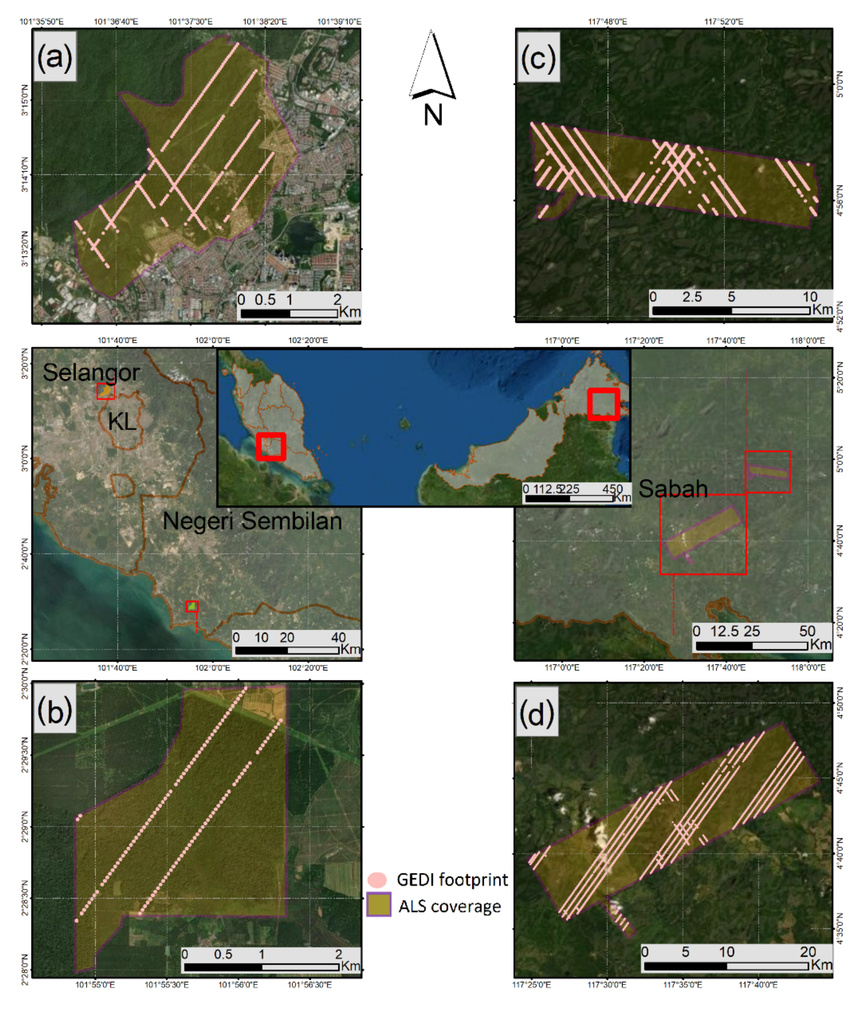
2.1. Study Sites

The forest sites pertinent to our study are shown in Figure 1. These include (a) a FRIM (Forest Research Institute Malaysia) forest site (Figure 1a), (b) Sungai Menyala Forest Reserve, Negeri Sembilan (Figure 1b), (c) Danum Valley Conservation Area (DVCA) (Figure 1c), and (d) the Stability of Altered Rainforest Ecosystem (SAFE) project site (Figure 1d). The FRIM site is located in the Forest Research Institute of Malaysia’s Selangor Forest Park (FRIM–SFP), Kepong, Selangor, Malaysia; it occupies an area of approximately 13 km2, and it is observed to include logged land forests, low land forests and hill forests. The elevation in this site varies from 50 to 296 m a.s.l. The Sungai Menyala Forest Reserve, Negeri Sembilan, is located at Port Dickson, Negeri Sembilan. The site is situated 5–6 km from the sea with an average ground elevation of 20–40 m a.s.l. The terrain in this site is flat, and the forest across this site is classified as a lowland dipterocarp-forest formation and Red Meranti–Keruing forest type [23,24]. The DVCA is a 75 km2 area of a relatively undisturbed lowland dipterocarp forest in Lahad Datu, Sabah, Malaysia. This site contains long-term experimental plots. The SAFE site is the subject of the Stability of Altered Forest Ecosystem project in east Sabah state, Malaysia. The site witnessed a progressive conversion from forest to palms, is characterized by high rainfall > 2000 mm/year and possesses various topographical landscapes [25]. Further description of the DVCA and SAFE sites and corresponding data can be found in [26,27,28].

2.2. Remote Sensing Data

2.2.1. Airborne Laser Scanning Data and Data Pre-processing

The ALS data over the two sites in the Malaysian peninsula were obtained from FRIM as LiDAR point clouds. The corresponding ALS surveys for these two sites were conducted in 2018 and 2016 for the FRIM and Negeri Sembilan sites respectively by FRIM at 600~1000 m flying altitude (depending on the site) and with an average point density of 8.5 points per m2. At the Sabah state sites, the data were acquired through a survey undertaken by the Natural Environment Research Council (NERC) Airborne Research Facility, UK, in 2014 using a Dornier 228–201 flown at 120–140 knots flight speed and altitude of 1400–2400 m a.s.l (depending on the site) [26,27,28]. The LiDAR data were preprocessed by NERC and made available at the Centre for Environmental Data Analysis (CEDA) archive [29]. The LiDAR point cloud processing was performed in R programming using the LidR package [30]. The relevant steps included filtering, classification for ground and surface returns and producing a canopy height model (CHM) at 1 × 1 m resolution. The CHM(s) over the four sites were utilized for the validation and selection of suitable GEDI metrics, resampling resolution and method to resample GEDI data as a proxy of the maximum canopy height over Malaysia.

2.2.2. GEDI Data

The GEDI spaceborne LiDAR system is orbiting on board the International Space Station with near-global coverage between 51.6° and −51.6° latitude. The instrument consists of three lasers, one of which is divided into two, and produces four beams dithered into eight-track ground transects. The illuminated shots are circular footprints of ~25 m in diameter spaced 60 m apart in the track direction and 600 m in the cross-track direction. The laser energy return is tracked as a function of time to generate geolocated waveforms, which are processed to several higher-level products by the GEDI team. The data products include L2A for height metrics, L2B for cover and vertical profile, L3A for gridded surface metrics and L4A and L4B for footprint and gridded aboveground biomass density [22,31]. The GEDI L2A [32] data product contains canopy relative height metrics rh (0–100) and has been made recently available on Google Earth Engine (GEE) [33]. All available data (April 2019 to September 2020) for both GEDI L2A first and second release (Version 1 and Version 2) were used for comparison with the ALS data. The V1 data were downloaded and preprocessed in R for all of Malaysia [34]. However, only GEDI V2 accessed on GEE after its recent release was used for further analysis due to its significant improvement in terms of accuracy and valid shots. The data were filtered using the quality and degradation flag provided in L2A bands. Measurements over non-forest areas were masked using Malaysian forest polygons provided by FRIM, and observations that were unlikely to be forest were filtered as outliers using the following thresholds: rh100 < 90 m and rh90 > 3 m. GEDI spatial coverage over the sites where ALS data were available is shown in Figure 1.

2.2.3. Climatic and Topographic Data

Multiple indices were selected as the potential climatic drivers of canopy height (Table 1). For the climatic variables, we used annual mean precipitation, annual mean temperature, the mean temperature of the wettest and driest quarter and the mean precipitation of the wettest month. All the climate data were obtained from the WorldClim dataset available in GEE [35]. The main proxy of water availability was calculated as the difference between the annual precipitation and the annual potential evapotranspiration [12,19]. This layer was generated using the annual potential evapotranspiration extracted from CIGAR’s recent global dataset release at 1 × 1 km. This recent dataset was chosen over other datasets due to its comparable spatial resolution and relative influence as shown in previous studies that used previous versions [36]. The topographic variables considered in this study were slope, aspect, mean curvature, Gaussian curvature, vertical, horizontal, max, and min curvature. The Shuttle Radar Topographic Mission Digital Elevation Model (SRTM-DEM) dataset was used to derive the relevant topographic characteristics at 1 × 1 km using the TAGEE package in GEE [37]. All included variables and relevant reference studies are listed in Table 1.

2.3. ALS and GEDI Canopy Height Comparison

In order to obtain comparable measurements from GEDI data and decide on the representative scale and metric as a proxy of canopy height over Malaysia tropical forest, different aggregation methods and resolution were explored for gridding and comparing GEDI and ALS data. Multiple grids of different resolutions (25, 30, 90, 250, 1000 m) were created to obtain comparable GEDI–ALS pairs. Both GEDI and ALS data were aggregated into these grids using several combinations shown in Table 2 to decide on the best-correlated GEDI metric and aggregation method to use for producing a GEDI-based canopy height map. To generate the map, 1 × 1 m CHM data over the considered sites were uploaded to the GEE, where all processing was conducted. The SAFE project area was divided into two sites to ease the computation of a large number of observations. The statistics used for comparison were: the coefficient of determination (R2), p, absolute (m) and relative (%) root mean square error (RMSE; rRMSE) and mean absolute error (MAE).

2.4. Canopy Height Modeling and Variables Importance

In order to rank the included variables and determine the most influential drivers of canopy height for further analysis, we utilized ML’s ability to fit the functional relationship between a response variable and multiple independent variables. Herein, our response variable was canopy height (m) derived from GEDI, and our predictor variables were the climate and topography variables described in Table 1. In random forest regression, variable importance is determined by averaging and normalizing the difference of the mean square error on the out-of-bag data for each tree before and after permuting a variable (i.e., as the decline in accuracy considering the permutation of variables) [39,40,41]. In the case of boosting, the importance is summed over each boosting iteration following the same calculation. All steps and processing are performed in R using the ‘caret’, ‘randomForest’ and ‘xgboost’ packages [41,42,43].

2.4.1. Machine Learning Algorithms

Primarily, two ML algorithms were used in this study. One was the random forest algorithm (RF), an ensemble ML that combines multiple decision trees created from bootstrapped datasets and considering subsets of variables in each step. The other algorithm used was the extreme gradient boosting tree (XGBTree), a regularized gradient boosting known for its efficiency and high performance [44]. The algorithm builds trees in sequence by predicting the residual based on the previous prediction, then prunes and adds to the previous trees based on adjustable hyperparameters. An additional implementation of XGB, the XGBDart, is also utilized in this study to provide additional insights as the dart base learner removes trees (dropout) during each round of boosting, allowing for more control over potential overfitting problems. The models have been chosen for their known high performance with nonlinear relationships, predictive ability and wide use in ecological models and forest application at fine, regional and global scales, e.g., [44,45,46,47,48].

2.4.2. Model Development and Feature Selection

The dataset was split into 80% training and 20% test data. Each model was trained using fivefold cross-validation fed by identical training data and then tested using the 20% validation set. A subset of 10% of the training data was used to develop the model and optimize the hyperparameters. Concerning the feature selection in this study, where screening the variable importance for ecological interpretation is the intended outcome of the model, the variables were tested for Pearson’s correlation coefficient. Backward elimination was used for eliminating spurious, non-informative and highly correlated variables one at a time considering the following criteria: Pearson’s correlation score, RF variable importance ranking, multiple regression p and model performance after removing the variable.
The number of trees and the number of predictors at each split were optimized at (500, 2) respectively for the RF model. For XGB, the optimized hyperparameters used in the final model for number of estimations, max_depth, learning and subsample were (1500, 6, 0.3, 1) respectively. The drop and skip rates for the XGB dart implementation were (0.1 and 0.5) respectively.

2.4.3. Model Validation

The models were evaluated using the test data and internally using the five k-fold cross-validation. The evaluation statistics were Pearson’s correlation (R), the coefficient of determination (R2), absolute (m) and relative (%) root mean square error (RMSE; rRMSE) and bias and mean absolute error (MAE).
RMSE = i = 1 n Y i ^   Y i 2 n ,
rRMSE = RMSE Y - × 100 ,
MAE = i = 1 n Y i ^   Y i n ,
where Y i ^ is the estimated canopy height, Y i is the observed canopy height; n is number of observations and Y - is the mean observed canopy height.

2.5. Exploring the Bivariate and Multivariate Relationships

2.5.1. Bivariate Relationships

The relationships between each of the most important predictors considered in the final model and the dependent variable (canopy height represented as the GEDI best correlated metric with ALS) was explored individually by fitting a generalized linear regression model (GLM) and power regression to the power of four. Moreover, the relationship between maximum observed canopy height and variable gradients was investigated by recording the maximum height found in all grid cells corresponding to each increment of each variable (0.1 °C for temperature, 1 mm for P-PET, 1 m for elevation, 0.1° for slope) and fitting GLM and power regression.
The relationship was examined separately for peninsular and eastern Malaysia, which was then followed by an analysis for all of Malaysia. Similar patterns were found for both Borneo and peninsular Malaysia considered separately.

2.5.2. Multivariate Relationships

For the multivariate analysis, two of the most important variables based on ranking were considered. Maximum canopy height observed for each 1 mm increment of water availability P-PET was plotted according to four elevation zones (0–500 m, 500–1000 m, 1000–1500 m, <1500 m), and the GLM and power regression model were fitted to explore the relationship. To gain further insights, a three-dimensional plot of GEDI canopy height, P-PET and elevation were illustrated, and three planes representing simplified ML models were fitted to examine the trend visually. The ML models were trained using the same training data and hyperparameters but considering only the two most important variables: P-PET and elevation.

3. Results

3.1. Comparison between ALS and GEDI-Derived Canopy Height

The number of GEDI shots considered over the Malaysian tropical forest area after filtration was 3,657,038, with an average spatial coverage of 22 pulses per km2. The average GEDI spatial coverage per km2 in the study sites ranged between 10.6 and 27.3 shots per km2 Table 3.
The multi-resolution and cross-aggregation comparison between GEDI-derived canopy height and ALS canopy height resulted in 60 pairs of comparisons for each site for each of the 5 GEDI considered metrics (rh50, rh75, rh90, rh95, rh100) as described previously in Table 2. The most consistent results, based on higher R2 and lower RMSE, occurred when comparing the ALS data gridded based on the 90th height percentile (HALS-90) and GEDI metric rh90. This pattern remained true when conducting the comparison for different GEDI aggregation methods and across the different resolutions. For all comparisons considered, the gridded GEDI rh90 metric compared with HALS-90 yielded a higher and more consistent correlation across all different comparison combinations and resolutions. The complete comparison results along with a summary of the statistics for GEDI coverage over each site can be found in the Supplementary Materials (Figures S1–S5). Therefore, GEDI rh90 aggregated using the 90th percentile was considered for further analysis.
Concerning the variation in R2 and RMSE across scales, 1 × 1 km had the highest correlations observed among all tested grid resolutions (Figure 2). A slight variation was observed between the finer resolutions of 25, 30 and 90 m across all sites. In contrast, for coarse resolution, a slight improvement for R2 to 250 m was followed by a significant increase for 1 × 1 km in all sites (except for the Negeri Sembilan site). RMSE witnessed a consistent decline as resolution became coarse across all sites.

3.2. Machine Learning-Derived Canopy Height Models

Concerning evaluating the statistical uncertainty of ML models in estimating canopy height, the three models performed relatively satisfactorily in terms of R2 and RMSE calculated based on the unseen 20% testing data. XGB Tree was the best performing model (R2 = 0.85, RMSE = 6.1 m) (Figure 3a). Considering the internal fivefold cross-validation of each model, RF explained 38% of the variance, while XGB Tree and DART explained 28% and 30% respectively. The three models reported variable importance consistently, with AMT, P-PET and elevation as the three most important explanatory variables. AMT ranked first in the XGB models, while P-PET ranked first in the RF models, with slight variations between the three important variables’ rankings in all models (Figure 3b).

3.3. Exploring the Bivariate and Multivariate Relationships

3.3.1. Bivariate Analysis for Canopy Height and Climatic Variables

In addition to the visual exploration of canopy height and each climatic variable, generalized regression models were fitted for assessing the relationship between canopy height and the annual mean temperature along with canopy height and P-PET. Moreover, the relationship of maximum canopy height for every 0.1 °C increment of temperature and for each 1 mm increment of P-PET was investigated in a similar manner. The same is illustrated in Figure 4.
The visual interpretation and the fitted models depict an association between canopy height and the mean annual temperature (Figure 4a). Concerning the relationship with the maximum canopy height, as depicted by the fitted models (R2 = 0.18, R2 = 0.5 for GLM models to the first and fourth orders, respectively), the lowest maximum height occurred where temperature is lower and increasing height is observed as the temperature increases. Peak is observed at ~26 °C, and a sharp decline is seen afterwards.
The distribution of canopy height per P-PET (Figure 4c) indicates that taller trees are associated with moderate P-PET (between 800–1750 mm). However, a less obvious linear relationship can be seen directly from canopy height and P-PET. For the relationship between maximum canopy height per 1 mm P-PET increment, the fitted curve (R2 = 0.54 for GLM model to the fourth order) depicts that maximum canopy height increases with P-PET to an upper threshold of ~800 mm and then decreases gradually for higher water supply. This is then followed by a sharp decrease after a certain breaking point representative of excessive water supply (~2700 mm). Tall trees occurred across all modest P-PET values, and a sharp decline in maximum tree height was observed at both ends of P-PET gradients (critical thresholds < 800 mm and >2700 mm) (Figure 4d).

3.3.2. Bivariate Analysis for Canopy Height and Topographical Variables

The relationships between each of the considered topographic variables and canopy height were evaluated independently taking the same approach as considered in the previous section. Figure 5 depicts those relationships. The fitted models and graph (Figure 5a) indicate a strong association between canopy height and elevation, with left-skewed distribution and the tallest trees observed at lower elevation gradients. A strong negative relationship between maximum canopy height and elevation increments was depicted in the fitted models (R2 = 0.52 and R2 = 0.58 for GLM models to the power of 1 and power of 4, respectively) (Figure 5a,b). The trend between maximum canopy height and elevation increments indicates that the negative association with higher elevation gradients starts at approximately 500 m as a breaking point. Canopy heights observed below 500 m were on average 4 m taller than those between 500 and 1000 m, 8 m taller than ones observed between 1000 and 1500 m and 28 m taller than those observed at altitudes above 1500 m.
The negative association between maximum canopy height and slope angle gradients indicates that taller trees occurred on flat land and shorter trees occurred on steeper slopes (Figure 5c,d). Topographic variable curvature and aspect are found to be less influential at the considered 1 × 1 km resolution. Weak associations are depicted between canopy height and topographic curvature, canopy height and canopy aspect (Figure 5e,f). Tall trees occur over all curvature gradients and in all aspect directions, with slight variation across the landscape.

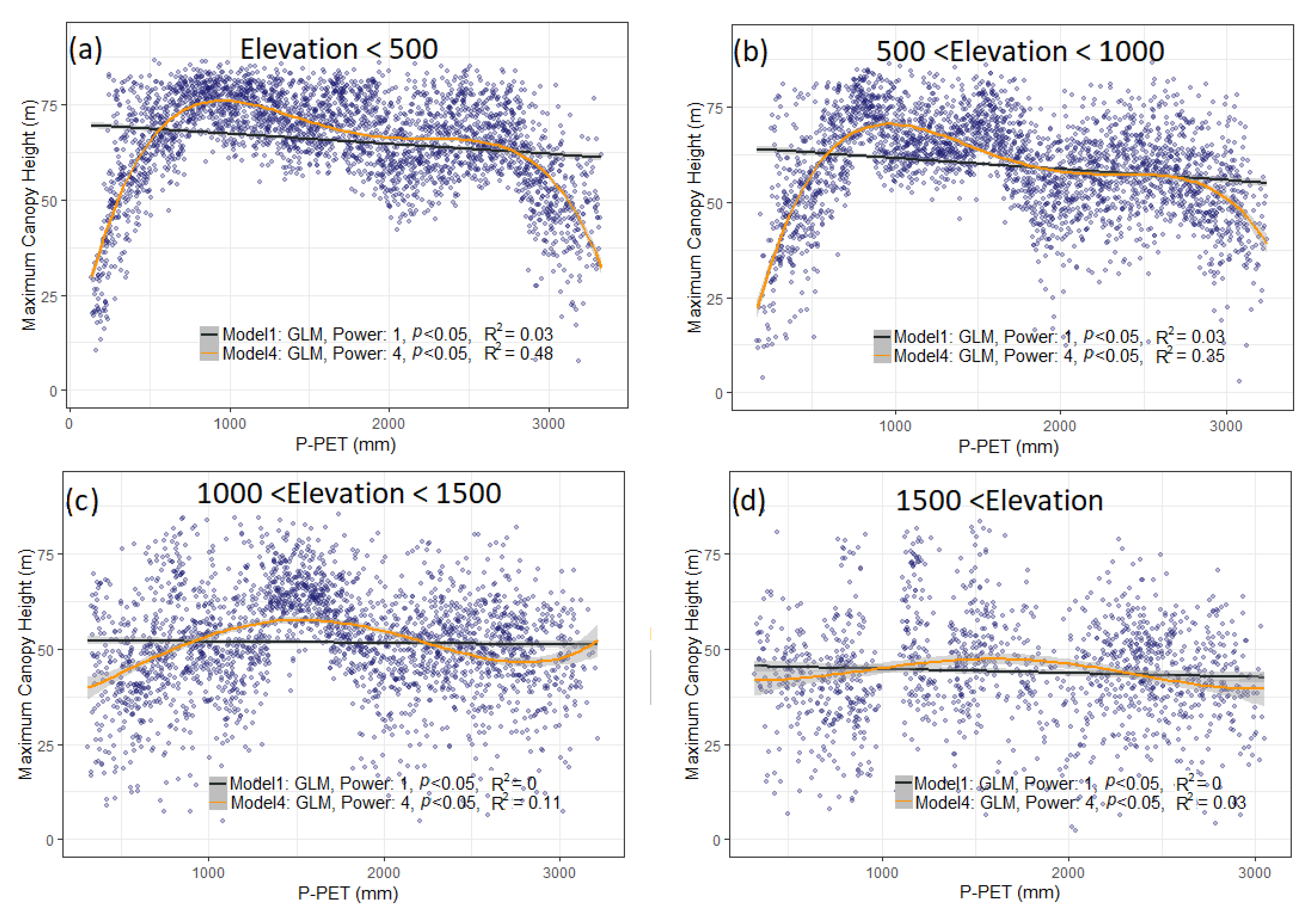
3.3.3. Multivariate Analysis for Canopy Height, Elevation and P-PET

The multivariate relationship between canopy height, elevation and P-PET were explored by partitioning the co-variables according to elevation intervals and fitting a separate model into each resulting canopy height–P-PET interval per elevation zone as illustrated in Figure 6.
The association between maximum canopy and P-PET was significant and strong at elevation 0–500 (R2 = 0.48 for GLM model power 4). This relationship was less significant for higher elevation intervals as it was found to be weakened into R2 = 0.35 for GLM model power 4 in the elevation zone between 500 and 1000 m; it then declined significantly after 1000 m before there was no observed relationship above 1500 m altitude.
To gain further insights into the multivariate relationships between canopy height, elevation and P-PET, the fitted ML models were plotted as a fit plane in three-dimensional plots for each of the three considered models (Figure 7). At the extreme ends of the elevation and water availability gradients, canopy height was found to be shorter. When both the water availability is extensive and the elevation is high, an obvious trend for shorter trees is shown. This trend was supported by the previous scatter plot of max canopy height aggregation per water availability gradient in different elevation zones.
The results corresponding to Borneo and Peninsular Malaysia are provided separately in the Supplementary Materials Figures S6 and S7.

4. Discussion

4.1. GEDI Validation and Resampling

In this study, we validated the GEDI relative height metrics (rh50, rh75, rh90, rh95, rh100) using different resampling approaches (mean, 90th percentile, max aggregation) over different spatial resolutions (GEDI footprint level, 30, 90, 250, 1000 m) to derive the representative proxy of maximum canopy height over the Malaysian tropical forest based on GEDI L2A data. The study confirmed that canopy height obtained from GEDI has a strong correlation with ALS data over the different sites, as shown in previous studies, and thus, it is useful to assess canopy height variation across landscapes [49,50,51,52,53].
The results showed that GEDI relative height metric rh90 compared with the HALS-90 was the most consistent among all compared pairs (Table 2) in terms of higher R2 and lower RMSE at all sites when comparing at the footprint level and at all sites among all used aggregation methods when comparing for coarse resolutions. Previous studies have considered such comparisons at footprint level where different GEDI rh metrics were considered and reported for different regions: rh95 in [51] globally, rh98 in [52], rh 95 in [45] and rh100 in [53] at regional scale. Moreover, differences in correlation using the same GEDI rh metric were also found when comparing different sites in the same region [53]. These inconsistencies could be due to site-specific factors such as canopy cover density, site homogeneity and topography (e.g., steep slope), which have the potential to interfere with the quality of recorded energy pulses [52,53,54,55]. This reported trend of lower estimation accuracy associated with steep slopes was observed in this study at the Danum Valley and FRIM sites where steep slopes are more common and lower R2 at footprint levels were found (Figure 2). Another reason for this variation in the estimated accuracy and/or the best correlated metric across the sites could be due to the differences in the data acquisition dates for ALS and GEDI data. This time difference could imply growth or disturbances changes [52,53]. For instance, an annual mean growth of 0.5 m could result in a 3 m error for a 6-year gap in data acquisition, which could be the case for the study sites in Sabah state. Finally, the increase in R2 for coarse resolutions (>90 m) when examining the correlations across multiple resolutions was consistent for all sites except Negeri Sembilan (Figure 2). This increase in R2 might be attributed to the inclusion of multiple GEDI measurements in the compared grid cells for coarse resolutions, which could mitigate the influence of the aforementioned factors affecting the accuracy, as well as any geolocation error. Regarding the considered resolution at 1 × 1 km, the influence of GEDI spatial coverage on the correlation strength between sites was examined in Figure 8. The lower GEDI coverage over the Negeri Sembilan site (~10 shots/km2) compared with other sites (>~22 shots/km2) explained the observed lower R2 for this site and indicated that higher accuracy is dependent on higher spatial coverage per grid cell. Such comparisons can be useful for similar future studies as they provide insights into determining a threshold for average shot per grid when resampling height maps at coarse resolution.
The results suggest that the correlation is highly dependent on the heterogeneity of the site, its topography and the spatial coverage of GEDI shots. Therefore, calibration with local data to determine the best correlated metric and region-specific consideration is suggested as an important process for deriving representative height at the intended scale.

4.2. Canopy Height Relationship with Climatic and Topographic Variables

In this study, we made use of three ML fitted models to gain insights into the strength of the functional relationships between canopy height and chosen variables and their relative importance [14,15,40,47,56]. The relatively significant and consistent values for R2 yielded from the three fitted models (Figure 3a) indicated strong relationships between forest heights and the studied variables. The findings from the ML models for variable importance (Figure 3b) show that canopy height is largely dominated by three variables: P-PET (proxy for water supply/availability), mean annual temperature and elevation. Ranking the most important variables based on the possible quantification of the predictor’s relative importance allowed us to focus the analysis on the most important variables [40,47,56]. This finding regarding the variable importance of water supply and temperature is in line with the tropical forest literature and the previous studies that accounted for similar scales in different regions [12,13,14,19,57].

4.2.1. Temperature

The observed association between temperature and canopy height in tropical forests is well-known as temperature is considered one of the major climatic factors of tropical forest structure and dynamic [57]. In line with the previous studies, the maximum canopy height increases as temperature increases to an observed threshold of 26 °C following which it declines sharply for extreme temperatures (Figure 4a,b). A similar trend and upper limit were reported previously on a global scale with a decline breakpoint at 25 °C [12].
In lowland tropical forests, temperature gradients experience little spatial variation [58]. Although this might indicate that the observed variation in maximum canopy height per temperature gradient could be driven by other factors rather than the temperature alone [12], it may also suggest that given the observed association with canopy height and the known relationship with forest dynamics, even a marginal increase in temperature may affect forest maximum height. Thus, for wider temperature gradients, such as in mountainous areas where temperature decreases at higher altitudes, the thermal range for species performance and distribution would be subject to an increase in temperature [57]. Whereas an increase of 2–3 °C is believed to drive many species out of their thermal range and to extinction in the current projections of global temperature increase [57,58,59]. Therefore, the suggested sensitivity of maximum canopy height variation to temperature changes could play a significant role in understanding and monitoring forest responses to climatic changes. This would be even more relevant for montane forests, where temperature gradients vary and could be impeded, among other key variables, into elevation gradients as discussed in Section 4.2.3.

4.2.2. Water Availability

The water availability proxy P-PET, described as the difference between annual precipitation and evapotranspiration, is observed to have a positive relationship with maximum canopy height up to a certain threshold before it becomes a negative relationship for excessive water supply.
This initial positive trend up to a certain threshold has been reported in many studies at different scales [19,60], while the negative decline after this threshold for excessive water supply was observed and reported in others [12]. Herein, the results confirm the findings of [12], who used space LiDAR to examine the same relationship on a global scale and inventory data at national scale; these authors depicted a peak of maximum height at 680 mm P-PET gradient (compared with 800 mm in our study) and a declining trend at higher P-PET. However, in contrast to the reported bell-shaped curve (R2 = 0.72) in [12], we observed a fourth-order curve fitted to maximum canopy height as the response variable of P-PET (R2 = 0.54) in this study. This fit depicts that although the maximum canopy height starts declining gradually after a comparable peak (~800 mm), the sharp decline occurs only after a much higher breaking point (~2700 mm) (Figure 4d).
The trend of decreasing canopy height with excessive water supply is explained in previous studies and has been attributed to the accompanied reduction of O2 in soil, root aerenchyma, [12,61,62], declines in the radiation inputs that affect photosynthesis [12,63] and cloudiness [12,57,64]. The latter is more relevant to tropical forests as high precipitation regions are often associated with persistent thick clouds that would reduce forest access to sunlight. This might partially explain the gradual trend of maximum canopy height decline for P-PET between the peak and breaking point before the effect of the aforementioned factors become more dominant for the excessive water supply. This could be investigated further by evaluating height variation trends near streams and water sources where water supply is not associated with precipitation. Nevertheless, this weak response to changes in the mediating water supply values between the peak and breaking point indicates the effect of other factors along with P-PET in controlling maximum canopy height variation.
The observed relationship involving diminishing maximum tree height at both ends of the P-PET gradients suggests the partial predictability of maximum tree height based on P-PET and hence, the usefulness of including P-PET in canopy height extrapolating models. This relationship and the identified critical thresholds of P-PET gradients (<800 mm and >2700 mm) could be useful to forest managers for monitoring forest response to precipitation and evapotranspiration changes and for the suitability analysis of forestation regions. Furthermore, it could also prove beneficial for the improvement of carbon-cycle and forest-growth models [12,63].

4.2.3. Topographic Variables

Tall trees were observed in all elevation gradients as expected, although trees were higher and more abundant in the lowlands areas (Figure 5a). These results depict a negative trend between maximum canopy height and higher elevation gradients after a breaking point at approximately ~500 m (Figure 5b and Figure S8). This trend and the negative association have been reported in many studies in tropical regions as well as in different forest biomes [14,15,57,65]. Elevation controls atmospheric pressure, temperature, cloudiness and many environmental changes tied to altitude such as drain, sunshine exposure, wind, soil and human land use [66,67,68]. Such trends are very likely to be attributed to these underlying variables such as temperature, which experiences a steady decrease at higher elevation and under greater cloud cover and wind exposure [57,65]. Decreasing availability of soil nutrients and water could partly also explain this decline [69].
Similar trends were found in previous studies, although breaking points were observed at different elevation levels. For example, in tropical regions, Clark et al. [57] found taller trees at altitudes less than 1000 m. Ameztegui et al. [65] studied montane forests in Spain and reported elevation breaking points at ~1600 m. Nevertheless, while the need for investigating the accurate position of such a breaking point is clear, exploiting its existence is of pivotal importance for monitoring mountain forest response to projected climatic changes as they provide the potential ability for isolating climatic effects from the other changes [65].
Topographic curvature (Figure 5e) and aspect (Figure 5f) are found to be less important in the case of the 1 × 1 km scale considered in our study. The influence of topographic curvature and aspect is found to decrease with scale [14]. Maximum canopy height decreased with increased slope (Figure 5c), and the tallest trees occurred at less steep slopes, contradicting previous studies. We acknowledge that the limitations associated with this study might affect the accuracy of the reported elevation breaking point and the relationship to topography. For instance, the considered scale in this study was 1 × 1 km, and a weak association between topographic variable and canopy height was reported for the coarse scale [14]. In addition, mountainous tropical landscapes are often characterized by steep slopes with large estimated areas of montane tropical forest at slope > 27 [70]. This might affect the quality of LiDAR data in such areas [52,53,54,55]. Additionally, considering the regional focus of this study, the distribution of forest height data with elevation data was left skewed due to the more abundant land and forest area in lower elevation zones.

4.2.4. The Multivariate Relationship between P-PET-Elevation

Considering the marginal differences in relative importance between the three highest ranked variables, and given the steady relationship between temperature and elevation, we considered only P-PET and elevation for this analysis. The relationship between maximum canopy height and P-PET according to elevation intervals (0–500 and 500–1000 m) was in line with the observed trend across all elevation gradients (Figure 6a,b). Interestingly, this relationship was weaker for higher elevation gradients above 1000 m and diminished for elevation gradients above 1500 m (Figure 6c,d). To gain additional insights into this interaction between the two most important variables, 3D planes were fitted to the multivariate relationship (Figure 7) based on the three implemented ML models [56]. The fitted planes for the three models confirmed the previously observed trend for shorter trees when both the water availability is extensive, and the elevation is high.
At the extreme elevation gradients and water availability gradients, canopy height was found to be shorter based on the three planes fitted on the ML models (Figure 7a–c). Nevertheless, the relationship between canopy height and water availability is depicted to be less significant for the extreme elevation values as illustrated in the scatter plot from max canopy height per P-PET gradient in the higher elevation zones (Figure 6d). The observed interrelationship contrasts the negative effect of extensive water supply at higher elevation, and the trend of shorter trees is most likely explained by the temperature limitation, which is one of the dominant factors controlled by elevation [19]. Whereas elevation and water supply together dominate the promotion of tallest trees [71], this trend suggests the intertwined use of the identified thresholds for both elevation and water availability to support the development of effective tools for monitoring the response of montane forest to climatic changes.

5. Conclusions

In this paper, we investigated the regional relationships and patterns of maximum canopy height across climatic and topographic variables focusing on elevation gradients and water availability and using a GEDI-derived canopy height map. Maximum canopy tree heights increase with increasing water supply up to a specific threshold (800 mm), decrease slightly for mediating gradients, and have a negative relationship above the breaking point of ~2700 mm. This pattern is found to be strong in an elevation zone below ~1000 m and starts to get weaker for higher altitudes, probably intertwined with the temperature limitation. These insights into this relationship along with the determined thresholds and breaking points could help with forest management practices, especially in regard to mountainous forest functioning, resilience, recovery and response to climate change. Simultaneously, this study demonstrates the power of GEDI in helping to better analyze the roles of the factors influencing canopy height variations and further comprehend biomass sequestration by different forest strata. Moreover, our investigation paves the way for future research endeavors to better understand the underlying patterns of other interactions between the environmental drivers, and therefore, developing efficient models at national and regional scales while simultaneously bridging the gap between theory, modeling and management, especially for montane forests.

Supplementary Materials

The following supporting information can be downloaded at: https://www.mdpi.com/article/10.3390/rs14133172/s1, Figure S1: GEDI-ALS comparison at 25 m resolution title; Figure S2: GEDI-ALS comparison at 30 m resolution title; Figure S3: GEDI-ALS comparison at 90 m resolution title; Figure S4: GEDI-ALS comparison at 250 m resolution title; Figure S5: GEDI-ALS comparison at 1000 m resolution title; Figure S6: Maximum canopy height per P-PET gradients for peninsular and Borneo part title; Figure S7: Maximum canopy height per elevation gradients for peninsular and Borneo part title; Figure S8: Maximum canopy height per elevation gradients across different elevation intervals title.

Author Contributions

All the authors have made a substantial contribution toward the successful completion of this manuscript. Conceptualization, W.S.W.M.J. and E.A.; methodology, W.S.W.M.J. and E.A.; software, E.A.; validation, E.A. and W.S.W.M.J.; formal analysis E.A.; investigation, E.A. and W.S.W.M.J.; data curation, E.A. and H.O.; writing—original draft preparation, E.A.; writing—review and editing, E.A., S.B., W.S.W.M.J., H.O., M.M., R.V.L., K.N.A.M., S.M.M., M.C.G.O., C.A.S. and A.C.; visualization, E.A.; supervision, W.S.W.M.J. and M.N.M.S.; funding acquisition, W.S.W.M.J. and H.O. All authors have read and agreed to the published version of the manuscript.

Funding

This research was funded by Research University Grant, GERAN UNIVERSITI PENYELIDIKAN with grant no: GUP-2021-073 and FUNDAMENTAL RESEARCH GRANT SCHEME with grant no: FRGS/1/2020/WAB03/UKM/02/1.

Institutional Review Board Statement

Not applicable.

Informed Consent Statement

Not applicable.

Data Availability Statement

The publicly available dataset analyzed in this study included data from NERC Airborne Research and Survey Facility (ARSF) Remote Sensing Data. NERC Earth Observation Data Centre that can be found at: [http://catalogue.ceda.ac.uk/uuid/55d1c9b6e7a4ce41b7a6f8416b7b6261]. The rasterized GEDI L2A: Google and USFS Laboratory for Applications of Remote Sensing in Ecology (LARSE) NASA GEDI mission, accessed through the USGS LP DAAC and made available in Google earth engine data catalog.

Acknowledgments

The authors would like to thank Forest Research Institute Malaysia (FRIM) for sharing the Airborne LiDAR data and field data for the study sites in peninsular Malaysia. We would also like to thank NERC Science of the Environment Airborne Research Facility, UK, for allowing access to the raw and processed LiDAR data downloaded from CEDA archive repositories. The authors would also like to thank the GEDI team and the NASA LPDAAC (Land Processes Distributed Active Archive Center) for providing GEDI data. The authors would also like to acknowledge and thank the two anonymous reviewers whose comments have helped to considerably improve the quality of the manuscript.

Conflicts of Interest

The authors declare no conflict of interest.

References

  1. Xu, P.; Zhou, T.; Yi, C.; Fang, W.; Hendrey, G.; Zhao, X. Forest Drought Resistance Distinguished by Canopy Height. Environ. Res. Lett. 2018, 13, 075003. [Google Scholar] [CrossRef] [Green Version]
  2. Keith, H.; Mackey, B.G.; Lindenmayer, D.B. Re-Evaluation of Forest Biomass Carbon Stocks and Lessons from the World’s Most Carbon-Dense Forests. Proc. Natl. Acad. Sci. USA 2009, 106, 11635–11640. [Google Scholar] [CrossRef] [Green Version]
  3. Lefsky, M.A.; Harding, D.J.; Keller, M.; Cohen, W.B.; Carabajal, C.C.; Del Bom Espirito-Santo, F.; Hunter, M.O.; de Oliveira, R., Jr. Estimates of Forest Canopy Height and Aboveground Biomass Using ICESat: ICESAT ESTIMATES OF CANOPY HEIGHT. Geophys. Res. Lett. 2005, 32. [Google Scholar] [CrossRef] [Green Version]
  4. Marselis, S.M.; Tang, H.; Armston, J.; Abernethy, K.; Alonso, A.; Barbier, N.; Bissiengou, P.; Jeffery, K.; Kenfack, D.; Labrière, N.; et al. Exploring the Relation between Remotely Sensed Vertical Canopy Structure and Tree Species Diversity in Gabon. Environ. Res. Lett. 2019, 14, 094013. [Google Scholar] [CrossRef]
  5. Xu, P.; Zhou, T.; Yi, C.; Luo, H.; Zhao, X.; Fang, W.; Gao, S.; Liu, X. Impacts of Water Stress on Forest Recovery and Its Interaction with Canopy Height. Int. J. Environ. Res. Public Health 2018, 15, 1257. [Google Scholar] [CrossRef] [PubMed] [Green Version]
  6. Dubayah, R.O.; Sheldon, S.L.; Clark, D.B.; Hofton, M.A.; Blair, J.B.; Hurtt, G.C.; Chazdon, R.L. Estimation of Tropical Forest Height and Biomass Dynamics Using Lidar Remote Sensing at La Selva, Costa Rica: FOREST DYNAMICS USING LIDAR. J. Geophys. Res. 2010, 115. [Google Scholar] [CrossRef]
  7. Dale, V.H.; Joyce, L.A.; Mcnulty, S.; Neilson, R.P.; Ayres, M.P.; Flannigan, M.D.; Hanson, P.J. Climate Change and Forest Disturbances: Climate Change Can Affect Forests by Altering the Frequency, Intensity, Duration, and Timing of Fire, Drought, Introduced Species, Insect and Pathogen Outbreaks, Hurricanes, Windstorms, Ice Storms, or Landslides. BioScience 2001, 51, 723–734. [Google Scholar] [CrossRef] [Green Version]
  8. Koch, G.W.; Sillett, S.C.; Jennings, G.M.; Davis, S.D. The Limits to Tree Height. Nature 2004, 428, 851–854. [Google Scholar] [CrossRef]
  9. Moles, A.T.; Warton, D.I.; Warman, L.; Swenson, N.G.; Laffan, S.W.; Zanne, A.E.; Pitman, A.; Hemmings, F.A.; Leishman, M.R. Global Patterns in Plant Height. J. Ecol. 2009, 97, 923–932. [Google Scholar] [CrossRef]
  10. Larjavaara, M.; Auvinen, M.; Kantola, A.; Mäkelä, A. Wind and Gravity in Shaping Picea Trunks. Trees 2021, 35, 1587–1599. [Google Scholar] [CrossRef]
  11. Wang, B.; Fang, S.; Wang, Y.; Guo, Q.; Hu, T.; Mi, X.; Lin, L.; Jin, G.; Coomes, D.A.; Yuan, Z.; et al. The Shift from Energy to Water Limitation in Local Canopy Height from Temperate to Tropical Forests in China. Forests 2022, 13, 639. [Google Scholar] [CrossRef]
  12. Tao, S.; Guo, Q.; Li, C.; Wang, Z.; Fang, J. Global Patterns and Determinants of Forest Canopy Height. Ecology 2016, 97, 3265–3270. [Google Scholar] [CrossRef]
  13. Zhang, J.; Nielsen, S.E.; Mao, L.; Chen, S.; Svenning, J.-C. Regional and Historical Factors Supplement Current Climate in Shaping Global Forest Canopy Height. J. Ecol. 2016, 104, 469–478. [Google Scholar] [CrossRef] [Green Version]
  14. Fricker, G.A.; Synes, N.W.; Serra-Diaz, J.M.; North, M.P.; Davis, F.W.; Franklin, J. More than Climate? Predictors of Tree Canopy Height Vary with Scale in Complex Terrain, Sierra Nevada, CA (USA). For. Ecol. Manag. 2019, 434, 142–153. [Google Scholar] [CrossRef] [Green Version]
  15. Farhadur Rahman, M.; Onoda, Y.; Kitajima, K. Forest Canopy Height Variation in Relation to Topography and Forest Types in Central Japan with LiDAR. For. Ecol. Manag. 2022, 503, 119792. [Google Scholar] [CrossRef]
  16. Dubayah, R.; Rich, P.M. Topographic Solar Radiation Models for GIS. Int. J. Geogr. Inf. Syst. 1995, 9, 405–419. [Google Scholar] [CrossRef]
  17. Geroy, I.J.; Gribb, M.M.; Marshall, H.P.; Chandler, D.G.; Benner, S.G.; McNamara, J.P. Aspect Influences on Soil Water Retention and Storage: ASPECT AND SOIL WATER RETENTION. Hydrol. Processes 2011, 25, 3836–3842. [Google Scholar] [CrossRef]
  18. Baldeck, C.A.; Harms, K.E.; Yavitt, J.B.; John, R.; Turner, B.L.; Valencia, R.; Navarrete, H.; Davies, S.J.; Chuyong, G.B.; Kenfack, D.; et al. Soil Resources and Topography Shape Local Tree Community Structure in Tropical Forests. Proc. Biol. Sci. 2013, 280, 20122532. [Google Scholar] [CrossRef]
  19. Klein, T.; Randin, C.; Körner, C. Water Availability Predicts Forest Canopy Height at the Global Scale. Ecol. Lett. 2015, 18, 1311–1320. [Google Scholar] [CrossRef]
  20. Simard, M.; Pinto, N.; Fisher, J.B.; Baccini, A. Mapping Forest Canopy Height Globally with Spaceborne Lidar. J. Geophys. Res. 2011, 116. [Google Scholar] [CrossRef] [Green Version]
  21. Liu, A.; Cheng, X.; Chen, Z. Performance Evaluation of GEDI and ICESat-2 Laser Altimeter Data for Terrain and Canopy Height Retrievals. Remote Sens. Environ. 2021, 264, 112571. [Google Scholar] [CrossRef]
  22. Dubayah, R.; Blair, J.B.; Goetz, S.; Fatoyinbo, L.; Hansen, M.; Healey, S.; Hofton, M.; Hurtt, G.; Kellner, J.; Luthcke, S.; et al. The Global Ecosystem Dynamics Investigation: High-Resolution Laser Ranging of the Earth’s Forests and Topography. Sci. Remote Sens. 2020, 1, 100002. [Google Scholar] [CrossRef]
  23. Abdul Razak, M.A.; Mohamed, M.; Alona, C.L.; Omar, H.; Misman, M.A. Tree Species Richness, Diversity and Distribution at Sungai Menyala Forest Reserve, Negeri Sembilan. IOP Conf. Ser. Earth Environ. Sci. 2019, 269, 012003. [Google Scholar] [CrossRef]
  24. Wyatt-Smith, J. Ecological Studies on Malayan Forests. Composition and Dynamic Studies in Lowland Evergreen Rain Forest in Two 5-Acre Plots in Bukit Lagong and Sungei Menyala Forest Reserves and in Two Half-Acre Plots in Sungei Menyala Forest; Research Pamphlet No. 101; Forest Research Institute, Forest Department: Kuala Lumpur, Malaysia, 1966. [Google Scholar]
  25. Nunes, M.; Ewers, R.; Turner, E.; Coomes, D. Mapping Aboveground Carbon in Oil Palm Plantations Using LiDAR: A Comparison of Tree-Centric versus Area-Based Approaches. Remote Sens. 2017, 9, 816. [Google Scholar] [CrossRef] [Green Version]
  26. Swinfield, T.; Both, S.; Riutta, T.; Bongalov, B.; Elias, D.; Majalap-Lee, N.; Ostle, N.; Svátek, M.; Kvasnica, J.; Milodowski, D.; et al. Imaging Spectroscopy Reveals the Effects of Topography and Logging on the Leaf Chemistry of Tropical Forest Canopy Trees. Glob. Chang. Biol. 2020, 26, 989–1002. [Google Scholar] [CrossRef] [PubMed] [Green Version]
  27. Swinfield, T.; Milodowski, D.; Jucker, T.; Michele, D.; Coomes, D. LiDAR Canopy Structure 2014, 2020 [Data set], Zenodo. Available online: https://doi.org/10.5281/zenodo.4020697 (accessed on 1 March 2022).
  28. Orme, D. Safe Web Safeproject.net. Available online: https://www.safeproject.net (accessed on 1 March 2022).
  29. CEDA Archive Web Browser. Available online: https://data.ceda.ac.uk/ (accessed on 1 March 2022).
  30. Roussel, J.-R.; Auty, D.; Coops, N.C.; Tompalski, P.; Goodbody, T.R.H.; Meador, A.S.; Bourdon, J.-F.; de Boissieu, F.; Achim, A. LidR: An R Package for Analysis of Airborne Laser Scanning (ALS) Data. Remote Sens. Environ. 2020, 251, 112061. [Google Scholar] [CrossRef]
  31. Duncanson, L.; Kellner, J.R.; Armston, J.; Dubayah, R.; Minor, D.M.; Hancock, S.; Healey, S.P.; Patterson, P.L.; Saarela, S.; Marselis, S.; et al. Aboveground biomass density models for NASA’s Global Ecosystem Dynamics Investigation (GEDI) lidar mission. Remote Sens. Environ. 2022, 270, 112845. [Google Scholar] [CrossRef]
  32. Dubayah, R.; Hofton, M.; Blair, J.; Armston, J.; Tang, H.; Luthcke, S. GEDI L2A Elevation and Height Metrics Data Global Footprint Level V002; NASA EOSDIS Land Processes DAAC: Greenbelt, MD, USA, 2021. [Google Scholar]
  33. Gorelick, N.; Hancher, M.; Dixon, M.; Ilyushchenko, S.; Thau, D.; Moore, R. Google Earth Engine: Planetary-Scale Geospatial Analysis for Everyone. Remote Sens. Environ. 2017, 202, 18–27. [Google Scholar] [CrossRef]
  34. R Core Team. R: A Language and Environment for Statistical Computing; R Foundation for Statistical Computing: Vienna, Austria, 2020; Available online: https://www.R-project.org/ (accessed on 1 March 2022).
  35. Fick, S.E.; Hijmans, R.J. WorldClim 2: New 1-km Spatial Resolution Climate Surfaces for Global Land Areas: NEW CLIMATE SURFACES FOR GLOBAL LAND AREAS. Int. J. Climatol. 2017, 37, 4302–4315. [Google Scholar] [CrossRef]
  36. Trabucco, A.; Zomer, R. Global Aridity Index and Potential Evapotranspiration (ET0); Climate Database; Figshare: Iasi, Romania, 2022; Volume 3. [Google Scholar] [CrossRef]
  37. Safanelli, J.; Poppiel, R.; Ruiz, L.; Bonfatti, B.; Mello, F.; Rizzo, R.; Demattê, J. Terrain Analysis in Google Earth Engine: A Method Adapted for High-Performance Global-Scale Analysis. ISPRS Int. J. Geoinf. 2020, 9, 400. [Google Scholar] [CrossRef]
  38. Zhu, J.; Shi, Y.; Fang, L.; Liu, X.; Ji, C. Patterns and Determinants of Wood Physical and Mechanical Properties across Major Tree Species in China. Sci. China Life Sci. 2015, 58, 602–612. [Google Scholar] [CrossRef]
  39. Strobl, C.; Boulesteix, A.-L.; Kneib, T.; Augustin, T.; Zeileis, A. Conditional Variable Importance for Random Forests. BMC Bioinformatics 2008, 9, 307. [Google Scholar] [CrossRef] [Green Version]
  40. Strobl, C.; Zeileis, A. Danger: High Power! Exploring the Statistical Properties of a Test for Random Forest Variable Importance; Universitätsbibliothek der Ludwig-Maximilians-Universität München: Munich, Germany, 2008. [Google Scholar] [CrossRef]
  41. Kuhn, M.; Wing, J.; Weston, S.; Williams, A.; Keefer, C.; Engelhardt, A.; Cooper, T.; Mayer, Z.; Kenkel., B. The Caret Package. Vienna, Austria, 2012. Available online: https://cran.r-project.org/package=caret (accessed on 1 March 2022).
  42. Liaw, A.; Wiener, M. Classification and Regression by random Forest. R News 2002, 2, 18–22. [Google Scholar]
  43. Chen, T.; Guestrin, C. XGBoost: A Scalable Tree Boosting System. In Proceedings of the 22nd ACM SIGKDD International Conference on Knowledge Discovery and Data Mining, San Francisco, CA, USA, 13–17 August 2016. [Google Scholar] [CrossRef] [Green Version]
  44. Arjasakusuma, S.; Swahyu Kusuma, S.; Phinn, S. Evaluating Variable Selection and Machine Learning Algorithms for Estimating Forest Heights by Combining Lidar and Hyperspectral Data. ISPRS Int. J. Geoinf. 2020, 9, 507. [Google Scholar] [CrossRef]
  45. Kacic, P.; Hirner, A.; Da Ponte, E. Fusing Sentinel-1 and -2 to Model GEDI-Derived Vegetation Structure Characteristics in GEE for the Paraguayan Chaco. Remote Sens. 2021, 13, 5105. [Google Scholar] [CrossRef]
  46. Anchang, J.Y.; Prihodko, L.; Ji, W.; Kumar, S.S.; Ross, C.W.; Yu, Q.; Lind, B.; Sarr, M.A.; Diouf, A.A.; Hanan, N.P. Toward Operational Mapping of Woody Canopy Cover in Tropical Savannas Using Google Earth Engine. Front. Environ. Sci. 2020, 8, 4. [Google Scholar] [CrossRef] [Green Version]
  47. Molnar, C. Interpretable Machine Learning. Github.io. Available online: https://christophm.github.io/interpretable-ml-book/ (accessed on 31 May 2022).
  48. Ross, C.W.; Hanan, N.P.; Prihodko, L.; Anchang, J.; Ji, W.; Yu, Q. Woody-Biomass Projections and Drivers of Change in Sub-Saharan Africa. Nat. Clim. Chang. 2021, 11, 449–455. [Google Scholar] [CrossRef]
  49. Francini, S.; D’Amico, G.; Vangi, E.; Borghi, C.; Chirici, G. Integrating GEDI and Landsat: Spaceborne Lidar and Four Decades of Optical Imagery for the Analysis of Forest Disturbances and Biomass Changes in Italy. Sensors 2022, 22, 2015. [Google Scholar] [CrossRef]
  50. Adrah, E.; Mohd Jaafar, W.S.W.; Bajaj, S.; Omar, H.; Leite, R.V.; Silva, C.A.; Cardil, A.; Mohan, M. Analyzing Canopy Height Variations in Secondary Tropical Forests of Malaysia Using NASA GEDI. IOP Conf. Ser. Earth Environ. Sci. 2021, 880, 012031. [Google Scholar] [CrossRef]
  51. Potapov, P.; Li, X.; Hernandez-Serna, A.; Tyukavina, A.; Hansen, M.C.; Kommareddy, A.; Pickens, A.; Turubanova, S.; Tang, H.; Silva, C.E.; et al. Mapping Global Forest Canopy Height through Integration of GEDI and Landsat Data. Remote Sens. Environ. 2021, 253, 112165. [Google Scholar] [CrossRef]
  52. Dorado-Roda, I.; Pascual, A.; Godinho, S.; Silva, C.; Botequim, B.; Rodríguez-Gonzálvez, P.; González-Ferreiro, E.; Guerra-Hernández, J. Assessing the Accuracy of GEDI Data for Canopy Height and Aboveground Biomass Estimates in Mediterranean Forests. Remote Sens. 2021, 13, 2279. [Google Scholar] [CrossRef]
  53. Adam, M.; Urbazaev, M.; Dubois, C.; Schmullius, C. Accuracy Assessment of GEDI Terrain Elevation and Canopy Height Estimates in European Temperate Forests: Influence of Environmental and Acquisition Parameters. Remote Sens. 2020, 12, 3948. [Google Scholar] [CrossRef]
  54. Hilbert, C.; Schmullius, C. Influence of Surface Topography on ICESat/GLAS Forest Height Estimation and Waveform Shape. Remote Sens. 2012, 4, 2210–2235. [Google Scholar] [CrossRef] [Green Version]
  55. Lang, N.; Kalischek, N.; Armston, J.; Schindler, K.; Dubayah, R.; Wegner, J.D. Global Canopy Height Regression and Uncertainty Estimation from GEDI LIDAR Waveforms with Deep Ensembles. Remote Sens. Environ. 2022, 268, 112760. [Google Scholar] [CrossRef]
  56. Yu, Q.; Ji, W.; Prihodko, L.; Ross, C.W.; Anchang, J.Y.; Hanan, N.P. Study Becomes Insight: Ecological Learning from Machine Learning. Methods Ecol. Evol. 2021, 12, 2117–2128. [Google Scholar] [CrossRef]
  57. Clark, D.B.; Hurtado, J.; Saatchi, S.S. Tropical Rain Forest Structure, Tree Growth and Dynamics along a 2700-m Elevational Transect in Costa Rica. PLoS ONE 2015, 10, e0122905. [Google Scholar] [CrossRef]
  58. Malhi, Y.; Silman, M.; Salinas, N.; Bush, M.; Meir, P.; Saatchi, S. Introduction: Elevation Gradients in the Tropics: Laboratories for Ecosystem Ecology and Global Change Research. Glob. Change Biol. 2010, 16, 3171–3175. [Google Scholar] [CrossRef]
  59. Chen, I.-C.; Hill, J.K.; Ohlemüller, R.; Roy, D.B.; Thomas, C.D. Rapid Range Shifts of Species Associated with High Levels of Climate Warming. Science 2011, 333, 1024–1026. [Google Scholar] [CrossRef]
  60. Givnish, T.J. Tree Diversity in Relation to Tree Height: Alternative Perspectives. Ecol. Lett. 2017, 20, 395–397. [Google Scholar] [CrossRef]
  61. Blom, C.W.; Voesenek, L.A. Flooding: The Survival Strategies of Plants. Trends Ecol. Evol. 1996, 11, 290–295. [Google Scholar] [CrossRef] [Green Version]
  62. Lambers, H.; Chapin, F.S., III; Pons, T.L. Plant Physiological Ecology, 2nd ed.; Springer: New York, NY, USA, 2008. [Google Scholar]
  63. Schuur, E.A.G. Productivity and Global Climate Revisited: The Sensitivity of Tropical Forest Growth to Precipitation. Ecology 2003, 84, 1165–1170. [Google Scholar] [CrossRef]
  64. Graham, E.A.; Mulkey, S.S.; Kitajima, K.; Phillips, N.G.; Wright, S.J. Cloud Cover Limits Net CO2 Uptake and Growth of a Rainforest Tree during Tropical Rainy Seasons. Proc. Natl. Acad. Sci. USA 2003, 100, 572–576. [Google Scholar] [CrossRef] [Green Version]
  65. Ameztegui, A.; Rodrigues, M.; Gelabert, P.J.; Lavaquiol, B.; Coll, L. Maximum Height of Mountain Forests Abruptly Decreases above an Elevation Breakpoint. GIsci Remote Sens. 2021, 58, 442–454. [Google Scholar] [CrossRef]
  66. Körner, C. The Use of “altitude” in Ecological Research. Trends Ecol. Evol. 2007, 22, 569–574. [Google Scholar] [CrossRef]
  67. Rumpf, S.B.; Hülber, K.; Klonner, G.; Moser, D.; Schütz, M.; Wessely, J.; Willner, W.; Zimmermann, N.E.; Dullinger, S. Range Dynamics of Mountain Plants Decrease with Elevation. Proc. Natl. Acad. Sci. USA 2018, 115, 1848–1853. [Google Scholar] [CrossRef] [Green Version]
  68. Körner, C.; Spehn, E. A Humboldtian View of Mountains. Science 2019, 365, 1061. [Google Scholar] [CrossRef] [Green Version]
  69. Hofhansl, F.; Wanek, W.; Drage, S.; Huber, W.; Weissenhofer, A.; Richter, A. Topography Strongly Affects Atmospheric Deposition and Canopy Exchange Processes in Different Types of Wet Lowland Rainforest, Southwest Costa Rica. Biogeochemistry 2011, 106, 371–396. [Google Scholar] [CrossRef]
  70. Spracklen, D.V.; Righelato, R. Tropical Montane Forests Are a Larger than Expected Global Carbon Store. Biogeosciences 2014, 11, 2741–2754. [Google Scholar] [CrossRef] [Green Version]
  71. Muscarella, R.; Kolyaie, S.; Morton, D.C.; Zimmerman, J.K.; Uriarte, M. Effects of topography on tropical forest structure depend on climate context. J. Ecol. 2020, 108, 145–159. [Google Scholar] [CrossRef]
Figure 1. ALS data sites and GEDI coverage over these sites: (a) FRIM FR site, Selangor, Peninsular Malaysia; (b) the Sungai Menyala FR site, Negeri Sembilan, Peninsular Malaysia; (c) the Danum Valley Conservation Area, Sabah, Malaysia; (d) SAFE project site, Sabah, Malaysia.
Remotesensing 14 03172 g001
Figure 2. GEDI–ALS comparison using the 90th percentile aggregation at all sites across different resolutions (25, 30, 90, 250, 1000 m) using RMSE (to the left) and R2 (to the right).
Remotesensing 14 03172 g002
Figure 3. (a) Models’ performance on the testing data: (a1) RF model; (a2) extreme gradient boosting tree; (a3) extreme gradient boosting Dart; (b) variable importance rankings for all models.
Remotesensing 14 03172 g003
Figure 4. Canopy height relationships with the climatic variables: (a) canopy height by mean annual temperature; (b) maximum canopy height per 1° increment of mean annual temperature; (c) canopy height by P-PET; (d) maximum canopy height per 1 mm increment of P-PET.
Remotesensing 14 03172 g004
Figure 5. Canopy height relationships by topographic variable: (a) canopy height by elevation; (b) maximum canopy height per 1 m increment of elevation gradient; (c) canopy height by slope; (d) maximum canopy height per 1° increments of slop gradients; (e) canopy height by topographic curvature; (f) Canopy height by topographic aspect.
Remotesensing 14 03172 g005
Figure 6. Maximum canopy height per 1 mm increment of P-PET gradient across different elevation zones: (a) elevation < 500; (b) 500 < elevation < 1000; (c) 1000 < elevation < 1500; (d) elevation > 1500.
Remotesensing 14 03172 g006
Figure 7. The canopy height–P-PET–elevation functional relationship as a plane fitted based on the three models: (a) RF; (b) XGB tree; (c) XGB Dart.
Remotesensing 14 03172 g007
Figure 8. R2 based on GEDI and ALS height correlation per average number of GEDI shots per 1 × 1 km cell across different sites.
Remotesensing 14 03172 g008
Table 1. Climate and topography variables.
IndicesResolutionReference StudiesSource of Used Dataset
Annual mean temperature (AMT) *
Mean temperature of wettest quarter (MTWQ)
Mean temperature of driest quarter (MTDQ)
Annual mean precipitation (AP)
Precipitation of the wettest month (PWM)
1 × 1 km[9,12,19,38]World Climate
Precipitation minus potential evapotranspiration (P-PET) *1 × 1 km[12,13,19]CIGAR
Elevation *
Slope *
Aspect *
Mean curvature *
Gaussian curvature
Vertical curvature
Horizontal curvature
Max/Min curvature
1 × 1 km[14,15]SRTM
Forest polygonsVector-FRIM
* The six variables that were included in the final model.
Table 2. GEDI and ALS aggregation combinations per grid resolution.
Grid Resolution25 m30, 90, 250, 1000 m
Considered GEDI metricsrh50, rh75, rh90, rh95, rh100rh50, rh75, rh90, rh95, rh100
GEDI GriddingNo aggregation;
comparison at footprint level
Max aggregation (rh-Max)
90th percentile (rh-90)
Mean (rh-Mean)
ALS GriddingMax aggregation (HALS-Max)
95th percentile (HALS-95)
90th percentile (HALS-90)
Mean (HALS-Mean)
Comparison statisticsR2
Mean absolute error (MAE)
Root mean square error (RMSE)
relative RMSE (rRMSE)
Table 3. GEDI coverage over the ALS data sites.
Study SitesPeninsular PartBorneo Part
FRIMNegeri SembilanDanumSAFE 1SAFE 2
Area (km2)12.96.675.5196.3200.3
GEDI shots (n)405 73 180736205128
Average GEDI shot per 1 km221.510.622.526.527.3
rh90 GEDI average height (m)25.73041.623.723
ALS average height (m)21.524.53314.618.8
Publisher’s Note: MDPI stays neutral with regard to jurisdictional claims in published maps and institutional affiliations.

