
Geodetic SAR for Height System Unification and Sea Level Research—Results in the Baltic Sea Test Network

 , , ,
, , ,  , , , and
Abstract
:
1. Introduction
2. Data Processing and Results for Individual Observation Types
2.1. SAR Data Analysis

| ECR | Ascending Image Sample | Descending Image Sample |
|---|---|---|
| Loksa | 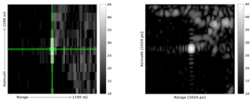 | 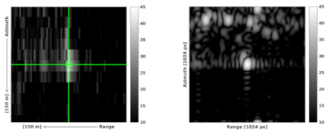 |
| Vergi | 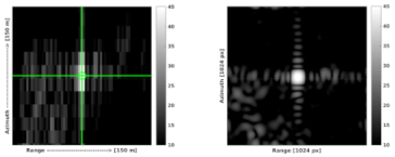 |  |
| Rauma | 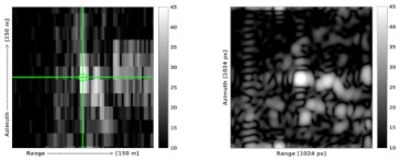 |  |
| Władys-ławowo |  | 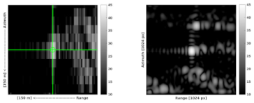 |
| Kobben |  |  |
| Vinberget | 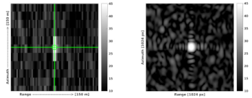 | 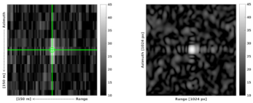 |
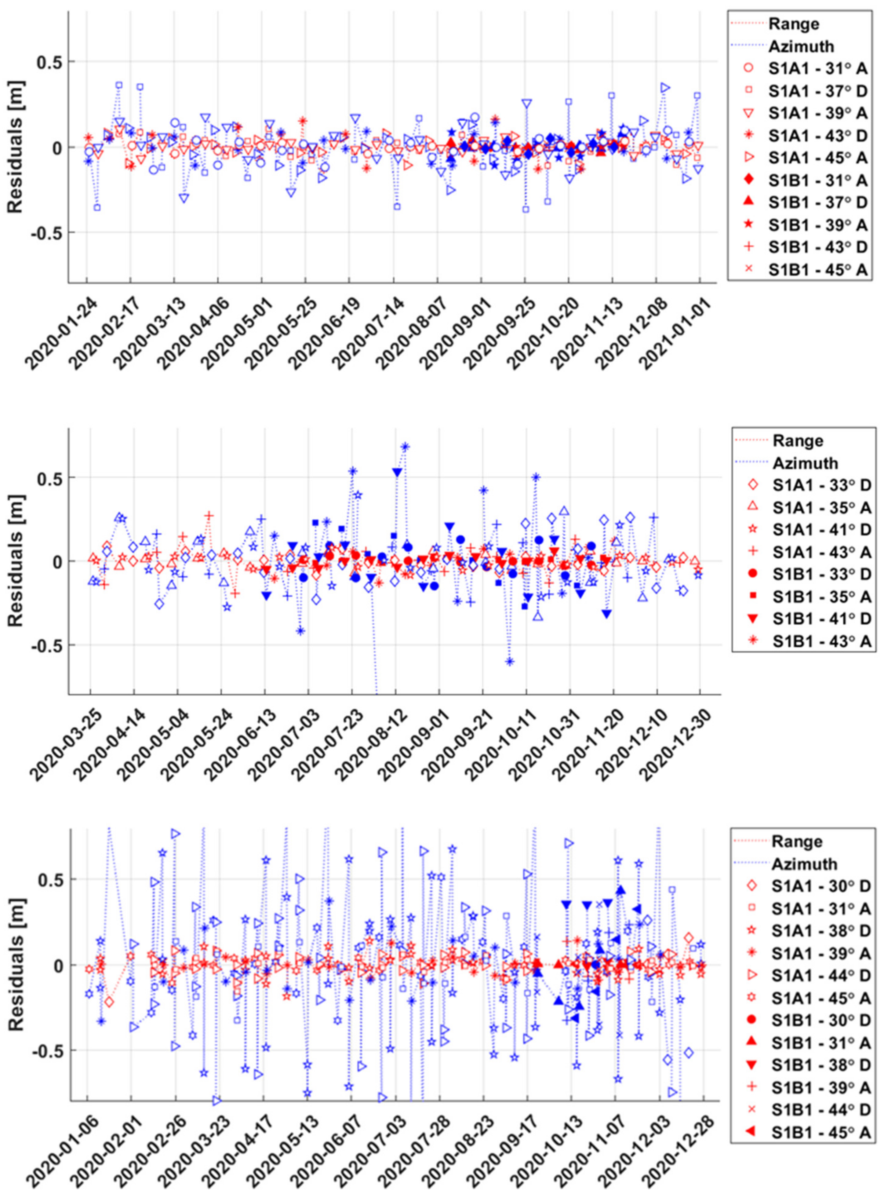
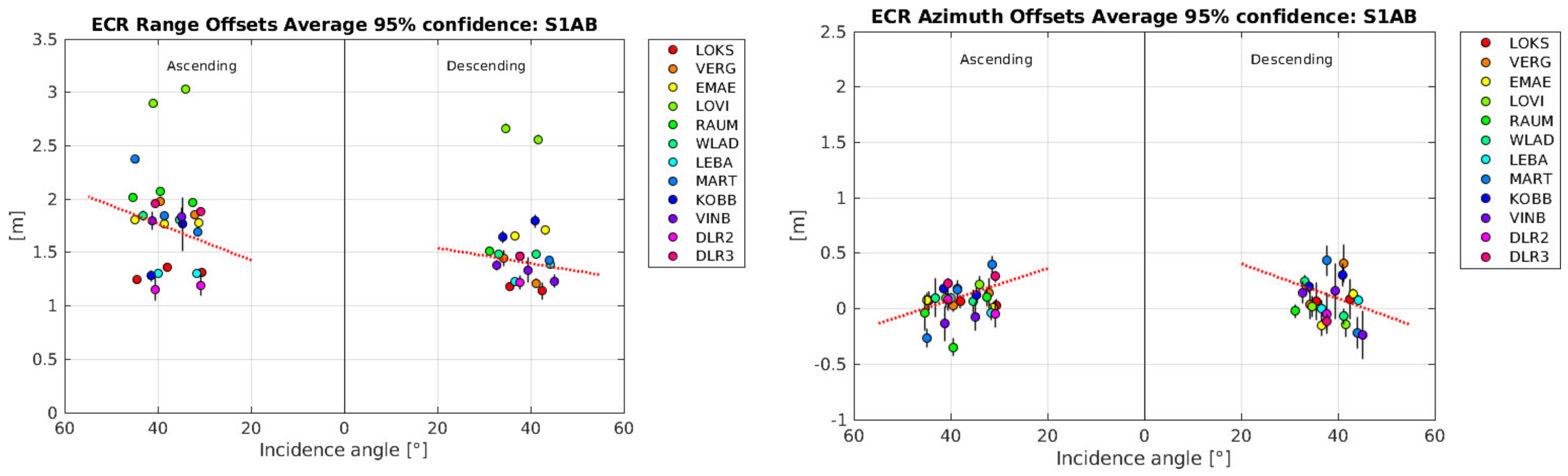
- The computation of range and azimuth residuals with respect to the surveyed ECR coordinates, applying the corrections for Sentinel-1 systematic effects, tropospheric and ionospheric delays and solid Earth tides. Note that the analysis is performed with the surveyed ECR origin coordinates corrected for the geometric ECR phase center offsets specified in the ECR manual for ascending and descending passes, following the methods proposed in [10]. The ECR origin coordinates are observed during installation with differential GNSS and are considered to be accurate within 5 cm or better depending on the instrumentation and observation time.
- The removal of outliers from the residuals of each individual geometry using the median and a 95% confidence interval, assuming normal distribution.
- The estimation of average ECR offsets from the cleaned residuals of each geometry along with the 95% confidence interval using least-squares methods.
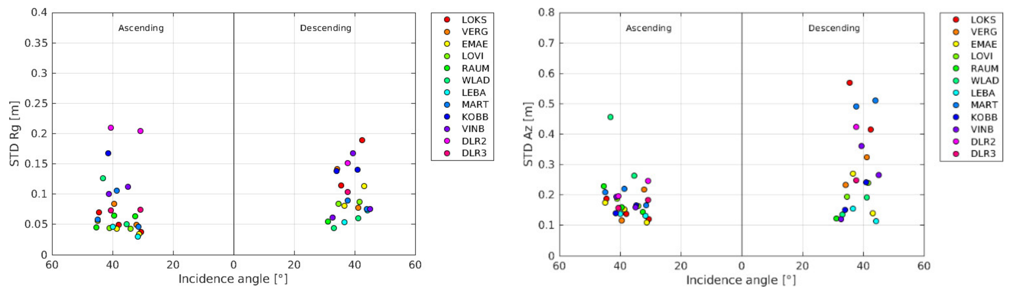
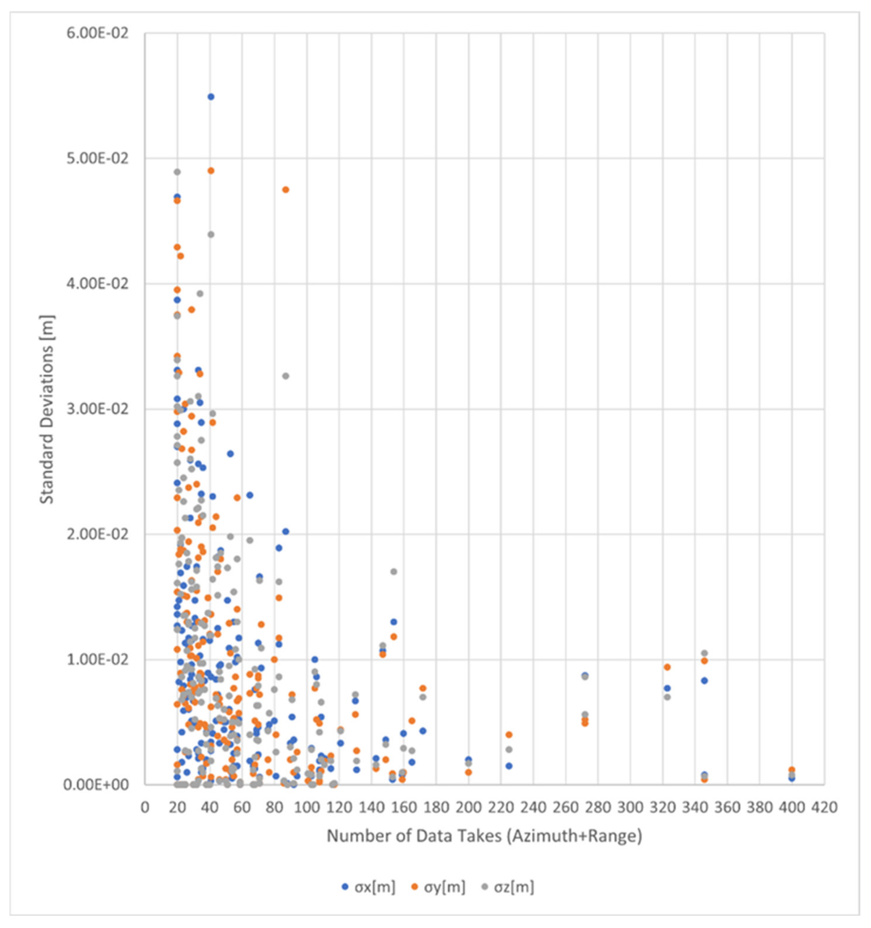
- The computation of the range and azimuth standard deviation for each set of residuals to empirically quantify the single observation precision (1 sigma) of each geometry.
2.2. SAR Positioning
2.3. GNSS Positioning
2.4. Tide Gauge Data Analysis
2.5. GOCE Based Geoid Determination
2.6. Reference Frames and Joint Standards
3. Absolute Sea Level and Height System Unification
3.1. Absolute Height Experiments
3.2. Baseline (Relative) Height Experiments
4. Data and Products, Summary and Conclusions, Future Work
4.1. Data and Products
4.2. Summary and Conclusions
4.3. Future Work
Author Contributions
Funding
Data Availability Statement
Acknowledgments
Conflicts of Interest
References
- Gruber, T.; Ågren, J.; Angermann, D.; Ellmann, A.; Engfeldt, A.; Gisinger, C.; Jaworski, L.; Marila, S.; Nastula, J.; Nilfouroushan, F.; et al. Geodetic SAR for Height System Unification and Sea Level Research—Observation Concept and Preliminary Results in the Baltic Sea. Remote Sens. 2020, 12, 3747. [Google Scholar] [CrossRef]
- Gisinger, C.; Balss, U.; Pail, R.; Zhu, X.X.; Montazeri, S.; Gernhardt, S.; Eineder, M. Precise Three-Dimensional Stereo Localization of Corner Reflectors and Persistent Scatterers with TerraSAR-X. IEEE Trans. Geosci. Remote Sens. 2015, 53, 1782–1802. [Google Scholar] [CrossRef]
- Bourbigot, M.; Johnsen, H.; Piantanida, R.; Sentinel-1 Product Definition. Technical Note by Sentinel-1 Mission Performance Center (MPC), Doc. S1-RS-MDA-52-7440, Iss. 2, Rev. 6, Date 22 July 2015. Available online: https://sentinels.copernicus.eu/web/sentinel/user-guides/sentinel-1-sar/document-library/-/asset_publisher/1dO7RF5fJMbd/content/sentinel-1-product-definition (accessed on 17 May 2022).
- Potin, P.; Gascon, F.; Stromme, A.; Zehner, C.; Wilson, H.; Figa, J.; Obligis, E.; Lindstrot, R. Sentinel High Level Operations Plan; ESA Technical Note, COPE-S1OP-EOPG-PL-15-0020, iss. 3, rev. 1; ESA: Frascati, Italy, 2021. [Google Scholar]
- Gisinger, C.; Schubert, A.; Breit, H.; Garthwaite, M.; Balss, U.; Willberg, M.; Small, D.; Eineder, M.; Miranda, N. In-Depth Verification of Sentinel-1 and TerraSAR-X Geolocation Accuracy using the Australian Corner Reflector Array. IEEE Trans. Geosci. Remote Sens. 2021, 59, 1154–1181. [Google Scholar] [CrossRef]
- Cumming, I.G.; Wong, F.H. Digital Processing of Synthetic Aperture Radar Data; Artech House: London, UK, 2005; ISBN 978-1-58053-058-3. [Google Scholar]
- Miranda, N.; Meadows, P.J. Radiometric Calibration of S-1 Level-1 Products Generated by the S-1 IPF; ESA Technical Document, Doc. ESA-EOPG-CSCOP-TN-0002, Iss. 1.0, Date 21 May 2015; ESA: Frascati, Italy, 2015. [Google Scholar]
- Schubert, A.; Miranda, N.; Geudtner, D.; Small, D. Sentinel-1A/B Combined Product Geolocation Accuracy. Remote Sens. 2017, 9, 607. [Google Scholar] [CrossRef] [Green Version]
- Hajduch, G.; Vincent, P.; Cordier, K.; Grignoux, M.; Husson, R.; Peureux, C.; Piantanida, R.; Recchia, A.; Francheschi, N.; Schmidt, K.; et al. S-1A & S-1B Annual Performance Report 2020; ESA Technical Document, Doc. MPC-0504, Iss. 1.1, Date 16 March 2021; ESA: Frascati, Italy, 2021. [Google Scholar]
- Czikhardt, R.; van der Marel, H.; Papco, J.; Hanssen, R.F. On the Efficacy of Compact Radar Transponders for InSAR Geodesy: Results of Multiyear Field Tests. IEEE Trans. Geosci. Remote Sens. 2022, 60, 1–13. [Google Scholar] [CrossRef]
- Dach, R.; Lutz, S.; Walser, P.; Fridez, P. (Eds.) Bernese GNSS Software Version 5.2. User Manual; Astronomical Institute, University of Bern, Bern Open Publishing: Bern, Switzerland, 2015; ISBN 978-3-906813-05-9. [Google Scholar] [CrossRef]
- Altamimi, Z.; Rebischung, P.; Metivier, L.; Collilieux, X. ITRF2014: A new release of the International Terrestrial Reference Frame modeling nonlinear station motions. J. Geophys. Res. Solid Earth 2016, 121, 6109–6131. [Google Scholar] [CrossRef] [Green Version]
- Petit, G.; Luzum, B. (Eds.) IERS Conventions 2010. 20210, Verlag des Bundesamts für Kartographie und Geodaäsie. Available online: https://iers-conventions.obspm.fr/ (accessed on 17 May 2022).
- Varbla, S.; Ågren, J.; Ellmann, A.; Poutanen, M. Treatment of tide gauge time series and marine GNSS measurements for vertical land motion with relevance to the implementation of the Baltic Sea Chart Datum 2000. Remote Sens. 2022, 14, 920. [Google Scholar] [CrossRef]
- Moritz, H. Advanced Physical Geodesy; Wichmann; Abacus Press: Karlsruhe, Germany; Tunbridge, UK, 1980; ISBN 978-3-87907-106-7. [Google Scholar]
- Tscherning, C.; Rapp, R.H. Closed Covariance Expressions for Gravity Anomalies, Geoid Undulations, and Deflections of the Vertical Implied by Anomaly Degree Variance Models; Report No. 208; Dep. Geod. Sci. Ohio State University: Columbus, OH, USA, 1974. [Google Scholar]
- Tscherning, C.C. Geoid Determination by 3D Least-Squares Collocation. In Geoid Determination: Theory and Methods; Sansò, F., Sideris, M.G., Eds.; Lecture Notes in Earth System Sciences; Springer: Berlin/Heidelberg, Germany, 2013; pp. 311–336. ISBN 978-3-540-74700-0. [Google Scholar]
- Forsberg, R. A Study of Terrain Reduction, Density, Anomalies and Geophysical Inversion Methods in Gravity Field Modeling; Dep. Geod. Sci. Ohio State University: Columbus, OH, USA, 1984. [Google Scholar]
- Sjöberg, L. Refined least squares modification of Stokes’ formula. Manuscr. Geod. 1991, 16, 367–375. [Google Scholar]
- Sjöberg, L.E.; Bagherbandi, M. (Eds.) Gravity Inversion and Integration—Theory and Applications in Geodesy and Geophysics; Springer International Publishing: Cham, Switzerland, 2017; ISBN 978-3-319-50298-4. [Google Scholar]
- Ågren, J.; Sjöberg, L.E.; Kiamehr, R. The new gravimetric quasigeoid model KTH08 over Sweden. J. Appl. Geod. 2009, 3, 143–153. [Google Scholar] [CrossRef]
- Ågren, J.; Strykowski, G.; Bilker-Koivula, M.; Omang, O.; Märdla, S.; Forsberg, R.; Ellmann, A.; Oja, T.; Liepins, I.; Parseliunas, E.; et al. The NKG2015 gravimetric geoid model for the Nordic-Baltic region. In Proceedings of the 1st Joint Commission 2 and IGFS Meeting International Symposium on Gravity, Geoid and Height Systems, Thessaloniki, Greece, 19–23 September 2016; Available online: https://www.isgeoid.polimi.it/Geoid/Europe/NordicCountries/GGHS2016_paper_143.pdf (accessed on 17 May 2022).
- Märdla, S.; Ågren, J.; Strykowski, G.; Oja, T.; Ellmann, A.; Forsberg, R.; Bilker-Koivula, M.; Omang, O.; Paršeliūnas, E.; Liepinš, I.; et al. From Discrete Gravity Survey Data to a High-resolution Gravity Field Representation in the Nordic-Baltic Region. Mar. Geod. 2017, 40, 416–453. [Google Scholar] [CrossRef]
- Förste, C.; Bruinsma, S.L.; Abrykosov, O.; Lemoine, J.-M.; Marty, J.C.; Flechtner, F.; Balmino, G.; Barthelmes, F.; Biancale, R. EIGEN-6C4 the latest combined global gravity field model including GOCE data up to degree and order 2190 of GFZ Potsdam and GRGS Toulouse. GFZ Data Serv. 2014. [Google Scholar] [CrossRef]
- Moritz, H. Geodetic Reference System 1980. J. Geod. 2000, 74, 128–162. [Google Scholar] [CrossRef]
- Förste, C.; Abrykosov, O.; Bruinsma, S.; Dahle, C.; König, R.; Lemoine, J.-M. ESA’s Release 6 GOCE gravity field model by means of the direct approach based on improved filtering of the reprocessed gradients of the entire mission. GFZ Data Serv. 2019. [Google Scholar] [CrossRef]
- Kvas, A.; Mayer-Gürr, T.; Krauss, S.; Brockmann, J.M.; Schubert, T.; Schuh, W.-D.; Pail, R.; Gruber, T.; Jäggi, A.; Meyer, U. The satellite-only gravity field model GOCO06s. GFZ Data Serv. 2019. [Google Scholar] [CrossRef]
- Forsberg, R.; Tscherning, C.C. An Overview Manual for the GRAVSOFT Geodetic Gravity Field Modelling Programs, 2nd ed.; 2008; Available online: https://www.academia.edu/9206363/An_overview_manual_for_the_GRAVSOFT_Geodetic_Gravity_Field_Modelling_Programs (accessed on 17 May 2022).
- Tscherning, C.C.; Rapp, R.H. Closed Covariance Expressions for Gravity Anomalies, Geoid Undulations, and Deflections of the Vertical Implied by Anomaly Degree Variance Models; Report No. 355; Dep. Geod. Sci. Ohio State University: Columbus, OH, USA, 1974. [Google Scholar]
- Mayer-Gürr, T.; Behzadpur, S.; Ellmer, M.; Kvas, A.; Klinger, B.; Strasser, S.; Zehentner, N. ITSG-Grace2018—Monthly, Daily and Static Gravity Field Solutions from GRACE. GFZ Data Serv. 2018. [Google Scholar] [CrossRef]
- Vestøl, O.; Ågren, J.; Steffen, H.; Kierulf, H.; Tarasov, L. NKG2016LU—A new land uplift model for Fennoscandia and the Baltic Region. J. Geod. 2019, 93, 1759–1779. [Google Scholar] [CrossRef] [Green Version]


| ECR Station | Active mm/dd-mm/dd | Passes [#] (Asc/ Desc) | Sent.-1 Obs. [#] | Acquired Obs. [#] | Success Rate [%] |
|---|---|---|---|---|---|
| Loksa (LOKS) | 02/14–09/12 12/28–12/31 | 3/2 | 171 | 164 | 95.61 |
| Vergi (VERG) | 03/03–08/01 12/28–12/31 | 3/2 | 81 | 81 | 100.00 |
| Emäsalo (EMAE) | 01/23–12/31 | 3/2 | 222 | 185 | 83.33 |
| Loviisa (LOVI) | 02/01–10/20 | 2/2 | 132 | 106 | 80.30 |
| Rauma (RAUM) | 04/21–12/31 | 2/2 | 142 | 76 | 53.52 |
| Władysławowo (WLAD) | 03/20–12/31 | 2/2 | 164 | 142 | 85.59 |
| Łeba (LEBA) | 05/15–12/31 | 2/2 | 141 | 116 | 82.27 |
| Mårtsbo (MART) | 01/07–12/31 | 3/3 | 322 | 218 | 67.70 |
| Kobben (KOBB) | 06/01–12/31 | 2/2 | 160 | 154 | 96.25 |
| Vinberget (VINB) | 10/01–12/31 | 2/3 | 57 | 57 | 100.00 |
| Oberpfaffenhofen (DLR2) | 01/10–02/25 06/17–09/01 | 2/1 | 85 | 85 | 100.00 |
| Oberpfaffenhofen (DLR3) | 01/10–12/31 | 2/1 | 177 | 177 | 100.00 |
| Configuration | a0 [s] | a1 [s/°] |
|---|---|---|
| ECR Range Delay Ascending | 7.2416 × 10⁻⁹ | 1.1405 × 10⁻¹⁰ |
| ECR Range Delay Descending | 1.1243 × 10⁻⁸ | −4.7810 × 10⁻¹¹ |
| ECR Azimuth Delay Ascending | 9.5494 × 10⁻⁵ | −2.102 × 10⁻⁶ |
| ECR Azimuth Delay Descending | 1.0584 × 10⁻⁵ | −2.3110 × 10⁻⁶ |
| ECR Station | Latitude [°] | Longitude [°] | Height [m] | Valid DTs [#] A/R | Epoch |
|---|---|---|---|---|---|
| Loksa | 59.582555692 | 25.705865677 | 20.0761 | 160/163 | 2020.475 |
| Vergi | 59.601493430 | 26.100800251 | 28.9661 | 66/77 | 2020.422 |
| Emäsalo | 60.203674412 | 25.625661421 | 34.2932 | 181/165 | 2020.586 |
| Loviisa | 60.440749584 | 26.284251613 | 46.8399 | 101/99 | 2020.508 |
| Rauma | 61.133538554 | 21.425982308 | 24.0824 | 75/72 | 2020.656 |
| Władysławowo | 54.796783467 | 18.418754840 | 34.6395 | 133/139 | 2020.639 |
| Łeba | 54.753658763 | 17.534876057 | 34.3894 | 116/109 | 2020.681 |
| Mårtsbo | 60.595133036 | 17.258527904 | 75.4769 | 206/194 | 2020.581 |
| Kobben | 60.409897086 | 18.230323460 | 25.6586 | 81/78 | 2020.586 |
| Vinberget | 62.373892667 | 17.427849782 | 149.6544 | 54/54 | 2020.852 |
| DLR2 | 48.084935323 | 11.281195447 | 626.6280 | 83/71 | 2020.542 |
| DLR3 | 48.087916451 | 11.279137080 | 623.8140 | 174/172 | 2020.517 |
| ECR Station | 1 M RMS | 2 M RMS | ||||
|---|---|---|---|---|---|---|
| dN [m] | dE [m] | dH [m] | dN [m] | dE [m] | dH [m] | |
| Loksa | 0.1617 | 0.2267 | 0.1724 | 0.0605 | 0.1702 | 0.1832 |
| Vergi | 0.1544 | 0.0817 | 0.0911 | 0.0667 | 0.1032 | 0.0920 |
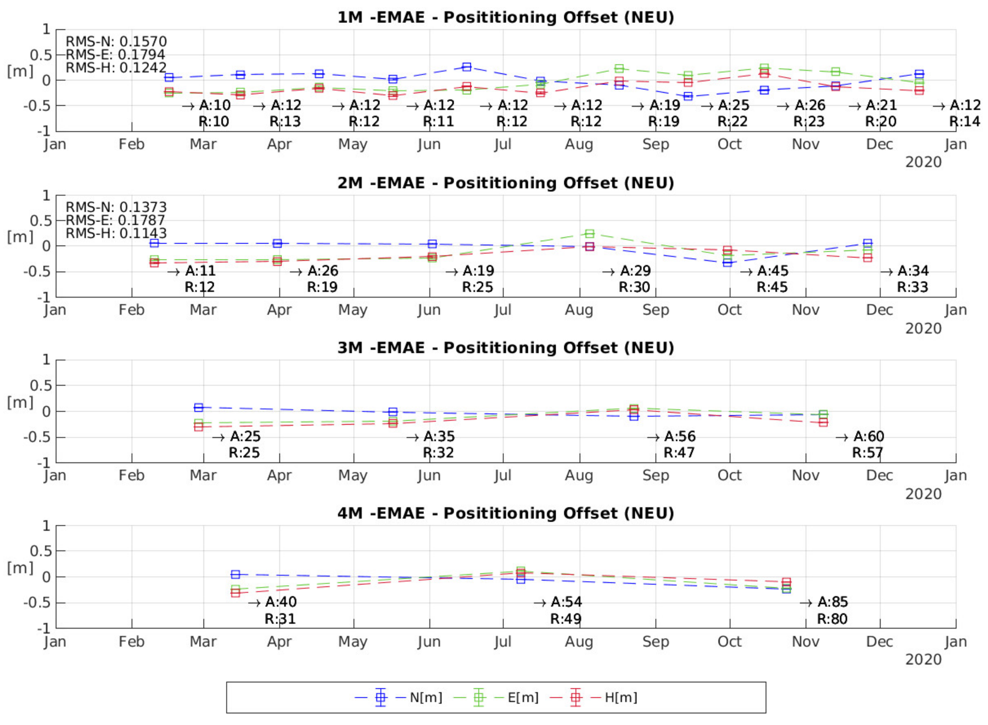
| Emäsalo | 0.1570 | 0.1794 | 0.1242 | 0.1373 | 0.1787 | 0.1143 |
| Loviisa | 0.1689 | 0.0647 | 0.1139 | 0.0999 | 0.1328 | 0.0620 |
| Rauma | 0.0797 | 0.0580 | 0.0359 | 0.0904 | 0.0394 | 0.0497 |
| Władysławowo | 0.2069 | 0.1272 | 0.1309 | 0.1482 | 0.2070 | 0.0725 |
| Łeba | 0.1300 | 0.1285 | 0.1201 | 0.0806 | 0.0883 | 0.0280 |
| Mårtsbo | 0.1470 | 0.0995 | 0.0889 | 0.2389 | 0.0292 | 0.0736 |
| Kobben | 0.1011 | 0.2485 | 0.1748 | 0.0840 | 0.2172 | 0.1269 |
| Vinberget | 0.0220 | 0.0549 | 0.0407 | - | - | - |
| DLR3 | 0.1348 | 0.3525 | 0.1275 | 0.0645 | 0.3165 | 0.1176 |
| Mean: | 0.1330 | 0.1474 | 0.1109 | 0.1071 | 0.1483 | 0.0920 |
| Min: | 0.0220 | 0.0549 | 0.0359 | 0.0605 | 0.0292 | 0.0280 |
| Max: | 0.2069 | 0.3525 | 0.1748 | 0.2389 | 0.3165 | 0.1832 |
| Median: | 0.1470 | 0.1272 | 0.1201 | 0.0872 | 0.1515 | 0.0828 |
| No Bias Correction applied for Loviisa and Kobben | ||||||
| GNSS Station | Latitude [°] | Longitude [°] | Height [m] |
|---|---|---|---|
| Łeba (LEBI) | 54.753775669 | 17.534799064 | 37.8856 |
| Loviisa (LOV3) | 60.440771458 | 26.283844394 | 49.8794 |
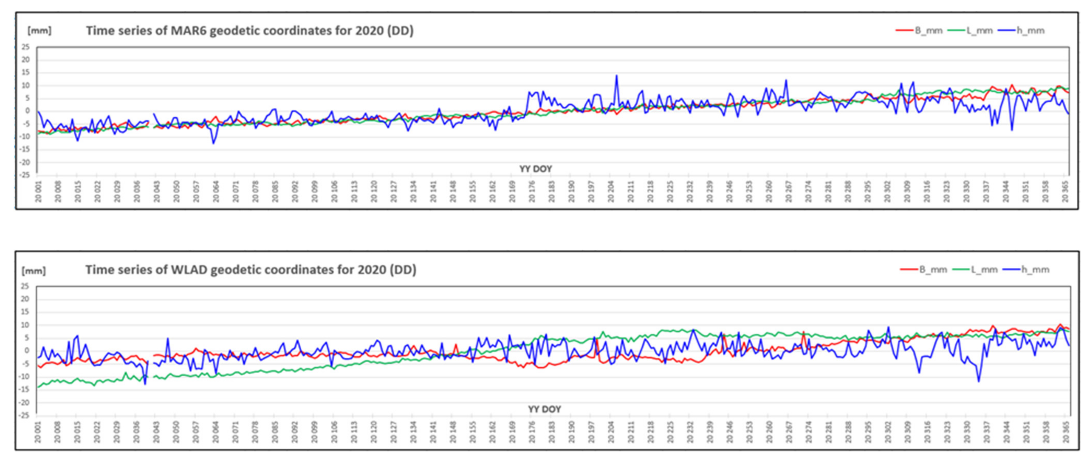
| Mårtsbo (MAR6) | 60.595145817 | 17.258531528 | 75.5578 |
| Vergi (VERG) | 59.601489744 | 26.100798661 | 30.0692 |
| Vinberget (VINB) | 62.373816278 | 17.427743125 | 150.2055 |
| Władysławowo (WLAD) | 54.796761422 | 18.418757500 | 34.7580 |
| TG Station | ECR Reference Height [m] | TG Average Sea Level Height [m] | STD TG Time Series [m] | Missing Data [%] |
|---|---|---|---|---|
| Loksa | 2.6385 | +0.343 | 0.245 | 1.2 |
| Emäsalo | 17.8155 | +0.338 | 0.238 | 0.6 |
| Rauma | 5.0075 | +0.258 | 0.216 | 1.1 |
| Kobben | 2.9606 | +0.188 | 0.200 | 0 |
| Vinberget | 123.5233 | +0.175 | 0.215 | 0 |
| Władysławowo | 5.6382 | +0.253 | 0.186 | 0.2 |
| Łeba | 3.0491 | +0.224 | 0.173 | 0.3 |
| Country | ECR Station | Quasi-Geoid Height [m] |
|---|---|---|
| Estonia | Loksa | 16.821 |
| Vergi | 16.555 | |
| Finland | Emäsalo | 15.509 |
| Loviisa | 15.453 | |
| Rauma | 19.096 | |
| Sweden | Kobben | 22.381 |
| Vinberget | 25.065 | |
| Mårtsbo | 24.627 | |
| Poland | Władysławowo | 28.883 |
| Łeba | 30.787 |
| ECR Station | Local Tie | Ellipsoidal Height [m] | Geoid Height [m] | Tide Gauge [m] | Ellipsoidal Height [m] |
|---|---|---|---|---|---|
| Władysławowo | TG, GNSS | +34.640 | +28.883 | +0.253 | +34.758 |
| Łeba | TG, GNSS | +34.389 | +30.787 | +0.224 | +37.886 |
| Vergi | GNSS | +28.966 | +16.555 | n/a | +30.069 |
| Loksa | TG | +20.076 | +16.821 | +0.343 | n/a |
| Emäsalo | TG | +34.293 | +15.509 | +0.338 | n/a |
| Loviisa | GNSS | +46.840 | +15.453 | n/a | +49.879 |
| Rauma | TG | +24.082 | +19.096 | +0.258 | n/a |
| Kobben | TG | +25.659 | +22.381 | +0.188 | n/a |
| Mårtsbo | GNSS | +75.477 | +24.627 | n/a | +75.558 |
| Vinberget | TG, GNSS | +149.654 | +25.065 | +0.175 | +150.206 |
| ECR Station | Local Tie | ECR to Tide Gauge [m] | GNSS to ECR [m] |
|---|---|---|---|
| Władysławowo | TG | −5.638 | n/a |
| Władysławowo | GNSS | n/a | −0.135 |
| Łeba | TG | −3.049 | n/a |
| Łeba | GNSS | n/a | −3.932 |
| Vergi | GNSS | n/a | −0.996 |
| Loksa | TG | −2.639 | n/a |
| Emäsalo | TG | −17.816 | n/a |
| Loviisa | GNSS | n/a | −3.574 |
| Rauma | TG | −5.007 | n/a |
| Kobben | TG | −2.961 | n/a |
| Mårtsbo | GNSS | n/a | −0.032 |
| Vinberget | TG | −123.523 | n/a |
| Vinberget | GNSS | n/a | −0.998 |
| ECR Station | Computed Ell. Height [m] | Observed Ell. Height [m] | Computed-Observed [m] |
|---|---|---|---|
| Władysławowo | +34.623 | +34.640 | −0.017 |
| Łeba | +33.954 | +34.389 | −0.435 |
| Vergi | +29.073 | +28.966 | +0.107 |
| Loviisa | +46.305 | +46.840 | −0.535 |
| Mårtsbo | +75.526 | +75.477 | +0.049 |
| Vinberget | +149.208 | +149.654 | −0.446 |
| ECR Station | Physical Height [m] | Absolute Sea Level [m] |
|---|---|---|
| Władysławowo | +0.119 | +0.372 |
| Łeba | +0.553 | +0.777 |
| Loksa | +0.616 | +0.959 |
| Emäsalo | −0.032 | +0.306 |
| Rauma | −0.021 | +0.237 |
| Kobben | +0.317 | +0.505 |
| Vinberget | +1.066 | +1.241 |
| Station A | Station B | Ell. Height Difference [m] | Ell. Height Difference [m] | Double Difference Ell. Height [m] |
|---|---|---|---|---|
| Władysławowo | Łeba | +3.128 | +3.546 | −0.418 |
| Władysławowo | Vergi | −4.689 | −4.813 | +0.124 |
| Władysławowo | Loviisa | +15.121 | +15.639 | −0.518 |
| Władysławowo | Mårtsbo | +40.800 | +40.734 | +0.066 |
| Władysławowo | Vinberget | +115.448 | +115.877 | −0.429 |
| Łeba | Vergi | −7.817 | −8.359 | +0.542 |
| Łeba | Loviisa | +11.993 | +12.093 | −0.100 |
| Łeba | Mårtsbo | +37.672 | +37.188 | +0.484 |
| Łeba | Vinberget | +112.320 | +112.331 | −0.011 |
| Vergi | Loviisa | +19.810 | +20.452 | −0.642 |
| Vergi | Mårtsbo | +45.489 | +45.547 | −0.058 |
| Vergi | Vinberget | +120.137 | +120.690 | −0.553 |
| Loviisa | Mårtsbo | +25.679 | +25.095 | +0.584 |
| Loviisa | Vinberget | +100.327 | +100.238 | +0.089 |
| Mårtsbo | Vinberget | +74.648 | +75.143 | −0.495 |
| Station A | Station B | Tide Gauge Height Difference [m] | Absolute Sea Level Height Difference [m] | Double Difference Sea Level [m] |
|---|---|---|---|---|
| Władysławowo | Łeba | −0.029 | +0.405 | −0.434 |
| Władysławowo | Loksa | +0.090 | +0.587 | −0.497 |
| Władysławowo | Emäsalo | +0.085 | −0.066 | +0.151 |
| Władysławowo | Rauma | +0.005 | −0.135 | +0.140 |
| Władysławowo | Kobben | −0.065 | +0.133 | −0.198 |
| Władysławowo | Vinberget | −0.078 | +0.869 | −0.947 |
| Łeba | Loksa | +0.119 | +0.182 | −0.063 |
| Łeba | Emäsalo | +0.114 | −0.471 | +0.585 |
| Łeba | Rauma | +0.034 | −0.540 | +0.574 |
| Łeba | Kobben | −0.036 | −0.272 | +0.236 |
| Łeba | Vinberget | −0.049 | +0.464 | −0.513 |
| Loksa | Emäsalo | −0.005 | −0.653 | +0.648 |
| Loksa | Rauma | −0.085 | −0.722 | +0.637 |
| Loksa | Kobben | −0.155 | −0.454 | +0.299 |
| Loksa | Vinberget | −0.168 | +0.282 | −0.450 |
| Emäsalo | Rauma | −0.080 | −0.069 | −0.011 |
| Emäsalo | Kobben | −0.150 | +0.199 | −0.349 |
| Emäsalo | Vinberget | −0.163 | +0.935 | −1.098 |
| Rauma | Kobben | −0.070 | +0.268 | −0.338 |
| Rauma | Vinberget | −0.083 | +1.004 | −1.087 |
| Kobben | Vinberget | −0.013 | +0.736 | −0.749 |
| Product Title | Product Description | Section |
|---|---|---|
| SAR Target Locations (PTA-RES) | Target range and azimuth location(s) from point target analysis. | Section 2.1 |
| SAR Raw Measurements (PTA-OBS) | SAR observation file generated from the point target analysis file. Processor specific corrections are applied to range and azimuth. | Section 2.1 |
| SAR Tropospheric Delays (COR-TD) | Tropospheric delays stored as one-way path delay in units of meters. | Section 2.1 |
| SAR Ionospheric Delay (COR-ID) | Ionospheric delays stored as one-way path delay in units of meters. | Section 2.1 |
| Geodynamic Corrections (COR-GC) | Geodynamic corrections to SAR range and azimuth observations due impact of solid Earth tidal deformations, ocean loading, atmospheric pressure loading, rotational deformation due to polar motion, ocean pole tide loading and secular trends. | Section 2.1 |
| Sentinel-1 Systematic Effects (COR-SC) | Sensor specific calibration constants and corrections to be applied to raw range and azimuth observations. | Section 2.1 |
| ECR Phase Center (COR-EC1) | Phase center shift of the ECR due to orbit geometry to be added as a correction to the observations. | Section 2.1 |
| ECR Electronic Delay (COR-EC2) | ECR electronics causes a signal delay to be corrected in the SAR measurements. | Section 2.1 |
| SAR Positions (SAR-POS) | Time series of coordinates of the SAR target as X, Y, Z coordinates in the ITRF2014 and uncertainties. | Section 2.2 |
| SAR Observation Residuals (SAR-OBS) | Time series of range and azimuth standard deviations and observation residuals. | Section 2.2 |
| GNSS Positions (GNSS-POS) | Coordinates of the GNSS stations as X, Y, Z coordinates in the ITRF2014 and uncertainties. | Section 2.3 |
| Sea Surface Height at TG (TG-SSH) | Corrected sea surface heights observed at TG with respect to TG benchmark. | Section 2.4 |
| Geoid Heights (GEO-HGT) | Geoid heights with mean epoch 2020.5 for the tide gauge stations. | Section 2.5 |
| Tide Gauge Heights (TG-HGT) | Average of unified physical heights of tide gauge stations. | Section 3.1 |
| Absolute Sea Level Heights (SL-ABS) | Average of absolute sea level heights of tide gauge stations. | Section 3.1 |
Publisher’s Note: MDPI stays neutral with regard to jurisdictional claims in published maps and institutional affiliations. |
© 2022 by the authors. Licensee MDPI, Basel, Switzerland. This article is an open access article distributed under the terms and conditions of the Creative Commons Attribution (CC BY) license (https://creativecommons.org/licenses/by/4.0/).
Share and Cite
Gruber, T.; Ågren, J.; Angermann, D.; Ellmann, A.; Engfeldt, A.; Gisinger, C.; Jaworski, L.; Kur, T.; Marila, S.; Nastula, J.; et al. Geodetic SAR for Height System Unification and Sea Level Research—Results in the Baltic Sea Test Network. Remote Sens. 2022, 14, 3250. https://doi.org/10.3390/rs14143250
Gruber T, Ågren J, Angermann D, Ellmann A, Engfeldt A, Gisinger C, Jaworski L, Kur T, Marila S, Nastula J, et al. Geodetic SAR for Height System Unification and Sea Level Research—Results in the Baltic Sea Test Network. Remote Sensing. 2022; 14(14):3250. https://doi.org/10.3390/rs14143250
Chicago/Turabian StyleGruber, Thomas, Jonas Ågren, Detlef Angermann, Artu Ellmann, Andreas Engfeldt, Christoph Gisinger, Leszek Jaworski, Tomasz Kur, Simo Marila, Jolanta Nastula, and et al. 2022. "Geodetic SAR for Height System Unification and Sea Level Research—Results in the Baltic Sea Test Network" Remote Sensing 14, no. 14: 3250. https://doi.org/10.3390/rs14143250