VENμS: Mission Characteristics, Final Evaluation of the First Phase and Data Production

Abstract

VENμS (Vegetation and Environment New micro (μ) Satellite) is a micro satellite launched in 2017 by the Israeli Space Agency (ISA) and the French Centre National d’Etudes Spatiales (CNES). VENμS is a research satellite containing two very different devices: an electric Hall effect thruster and a multispectral optical camera. This paper focuses on the multispectral camera. The camera provides images at a resolution of 5 m, with a field of view of 27 km, and the orbit of the satellite was chosen to allow us to revisit of each observed site with constant angles every second day. In November 2020, VENμS ended the first phase of its mission. This phase, called VM01, allowed us to provide about 150 accurate time series over selected scientific sites over almost three years. Extensive work was conducted to calibrate the camera and assess the quality of the products. Not everything worked as planned before launch and a large amount of work was necessary to correct some defects of the camera or to improve the geometric registration of images. This article establishes the image quality VM01 final assessment including the presentation of radiometric and geometric calibration methods, the estimation of instrument performances and their associated temporal stabilities and the monitoring activities. In addition, it highlights the whole mechanism of data programming, reception and production. The end of VM01 phase is not the end of the VENμS mission, and a new phase started on a one-day repeat orbit.

1. Introduction

The VENμS mission (Vegetation and Environment New micro (μ) Satellite) was designed in 2002 in the framework of a collaboration between the Israeli Space Agency (ISA) and the French Centre National d’Etudes Spatiales (CNES). At that time, it was very difficult to obtain high ground resolution time series of cloud free images with a revisit period of a couple of days, under similar observation geometries to minimize directional effects [1]. The only repetitive time series with constant viewing angles was provided by geo-stationary satellites, but at a spatial resolution of a few kilometers. Some wide field of view scanners such as AVHRR [2], SPOT/VEGETATION [3] or MODIS [4] provided daily observation time series with resolutions of 1 km or more, but only under very different viewing angles. In order to demonstrate the potential of repetitive imagery with constant view angles at a high resolution, the French space agency CNES promoted the concept of a daily imager with constant view angles [5]. After it was decided to build this mission in collaboration between France and Israel, the concept evolved to a two-day revisit mission to allow the observation of both France and Israel. Due to different technical difficulties, the VENμS satellite was finally launched in 2017 [6].

VENμS is an Earth observation satellite developed in cooperation by France and Israel and launched on 2 August 2017. It aims at acquiring time series with frequent observations (every second day) under constant viewing angles, at a high resolution (5 m), over land and coastal scientific sites to improve the understanding and modelling of natural processes. These images are acquired by a radiometer provided by CNES. In addition, to the scientific mission, VENμS has a technological mission with two small thrusters based on Hall effect, called IHET for Israeli Hall Effect Thruster. The thrusters are used to change and maintain the VENμS orbit. This technological mission is entirely managed by the Israeli team of VENμS project (Figure 1).

During VM01 phase, VENμS satellite was on a low earth orbit at 720 km. This orbit was sun synchronous with an inclination of 98.27°, crossing the equator at 10:30 local time. These specific orbit parameters were chosen to improve the revisit cycle compared to other similar Earth observation mission such as Sentinel 2 or Landsat 8. Indeed, VENμS provides images every two days over a set of scientific sites with constant viewing angles.

In order to obtain a maximal uptake of VENμS data by users, it was decided to deliver a complete set of products available on a free and open basis, to spare users with the burden of all preprocessing tasks. Designed as soon as 2008, these products constituted the precursors of the Analysis Ready Data [7]. A Level-1 product provides ortho-rectified time series with the same geometrical sampling grid for all acquisition dates for a given time series. The data are expressed as top-of atmosphere reflectances. The Level-2 product uses the same grid as the Level-1, but provides surface reflectances after atmospheric correction, with a high-quality cloud and cloud shadows mask. The Level-3A provides bi-weekly syntheses of cloud free surface reflectances obtained using a weighted average of all cloud free surface reflectances gathered during a fortnight.

Firstly, this article briefly presents the instrument characteristics and the different VENμS product levels before describing all the radiometric and geometric calibration methods used for the monitoring of the complete set of image quality parameters and performances. Then, it details the mission programming and the whole chain of data reception. Finally, information about data production is given, also explaining the way image quality is monitored. Some statistics on the production of the entire VM01 archive are also provided.

2. Calibration and Performances of the Instrument

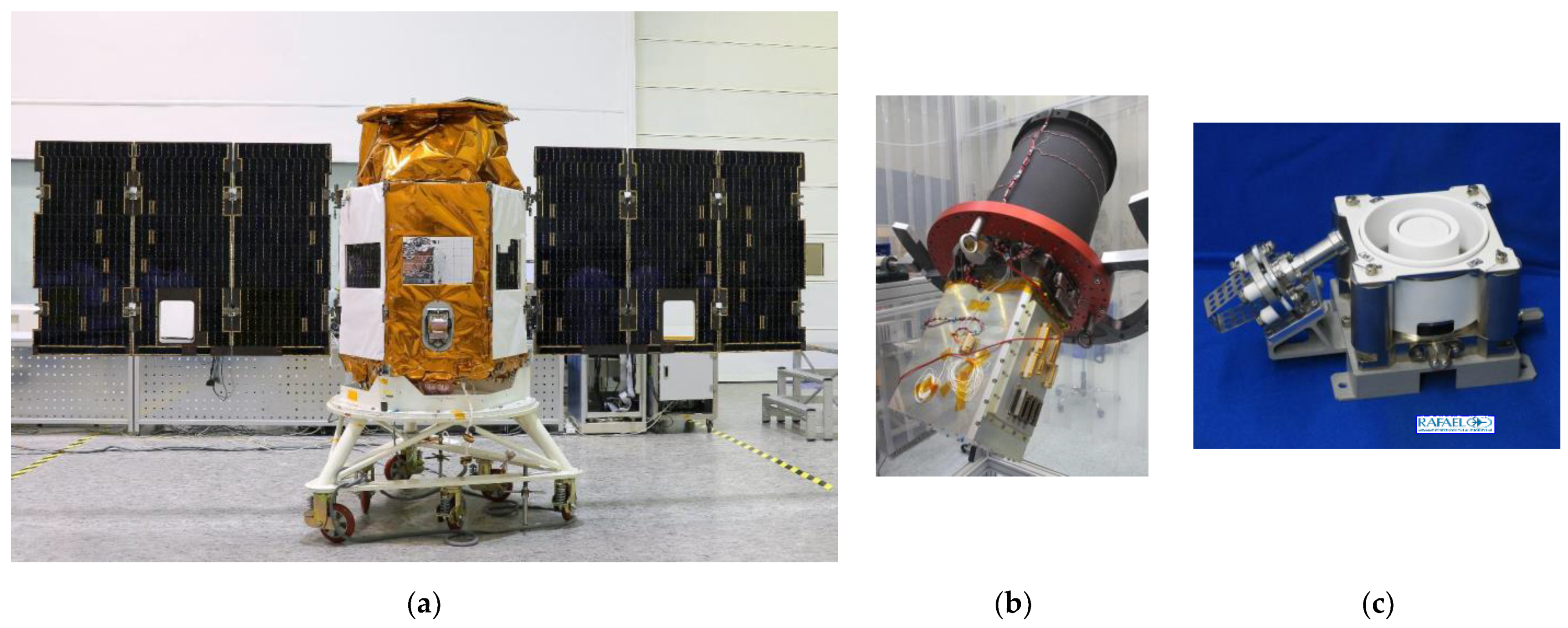
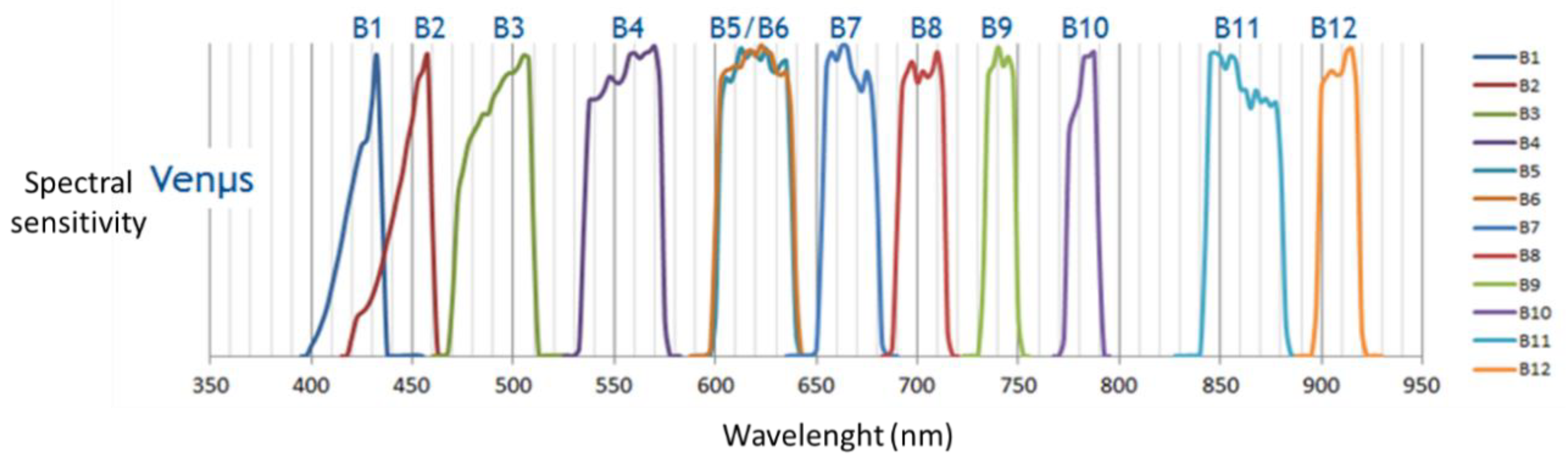
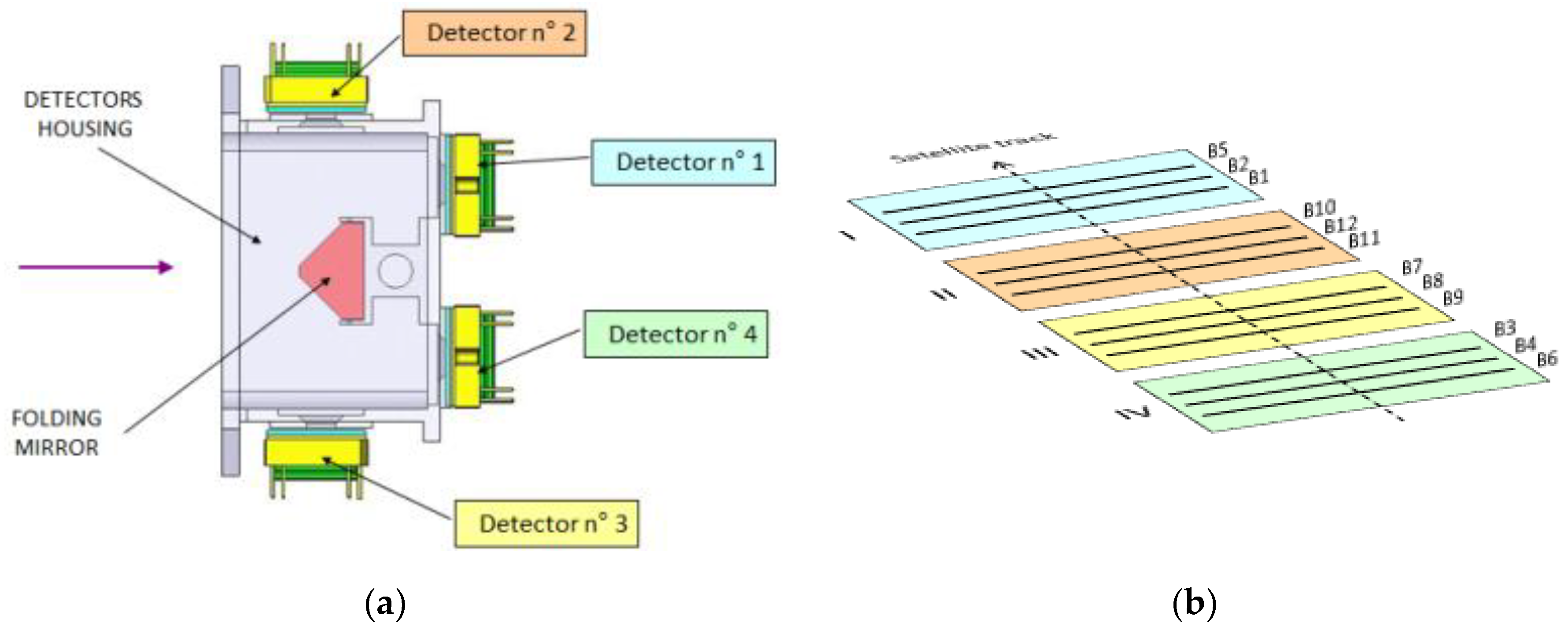
2.1. Key Features

The focus here is on the VENμS radiometer. This instrument is dedicated for the scientific mission. The VENμS radiometer allows us to acquire images with 12 spectral bands in the visible and near infrared with a ground nadir resolution of 5.3 m. The swath of 27 km and especially the 2-day revisit are the added values of VENμS satellite. The two next figures (Figure 2 and Figure 3) present VENμS spectral bands and the focal plane design.

A total of 11 filters were designed from 420 nm to 910 nm for specific studies about vegetation cycle, atmospheric corrections (water vapor and aerosol characterization) and water color. One specificity of VENμS is the duplication of the 620 nm spectral band. Indeed, two bands (B5 and B6) have been centered at 620 nm but with a 1.5° observation angle difference. The Figure 3 shows that the spectral bands B5 and B6 are to the ends of the focal plane. This observation angle difference allows us to determine the altitude of pixels for detecting clouds or creating digital elevation model (DEM) creation.

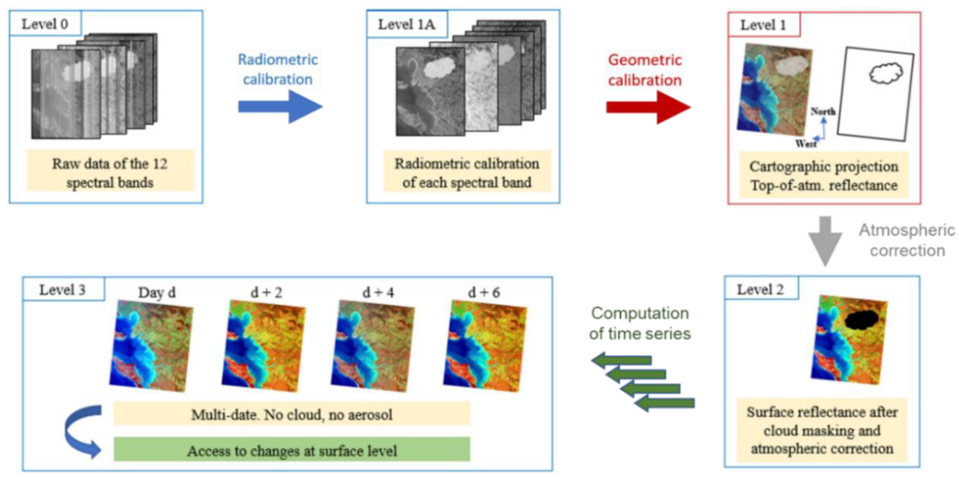
2.2. VENμS Products Levels and Production Processings

The different VENμS level products are detailed hereafter and illustrated in the Figure 4.

The Level-0 product contains decompressed raw data with additional information included to prepare Level-1 processing. This level is the basis archive product.

The Level-1A product is derived from the Level-0 after the application of radiometric corrections: interpolation of defective pixels, equalization, stray light and polarization sensitivity corrections. This product has the same geometry than the Level-0 (raw geometry). Level-0 and Level-1A are not distributed.

The Level-1 product is obtained after geometric calibration and conversion into top of atmosphere reflectance product (absolute radiometric calibration). These products are available for scientists on the THEIA data service center (https://www.theia-land.fr/en/product/venus/, accessed date: 21 June 2022). The geometric calibration includes location model refining, inter-band registration, computation of location grid for each spectral band and spatial resampling for all spectral bands into a cartographic projection. The Level-1 provides a geolocated top of the atmosphere reflectance with a subpixel multidate registration, a cloud mask and geometric quality indexes. The spatial resolution is 5 m.

The Level-2 product, which also has a resolution of 5 m, contains a fine cloud mask, surface reflectances after atmospheric corrections and slope effects correction for all spectral bands and aerosol optical thickness (AOT) values retrieved at a reduced resolution.

The Level-3 product is generated by creating a composite image from the Level-2 products every 15 days. This product provides an average of cloud free surface reflectances gathered during the compositing period which is longer than the period between two Level-3 products.

2.3. Calibration and Performances of Level-1 VENμS Products

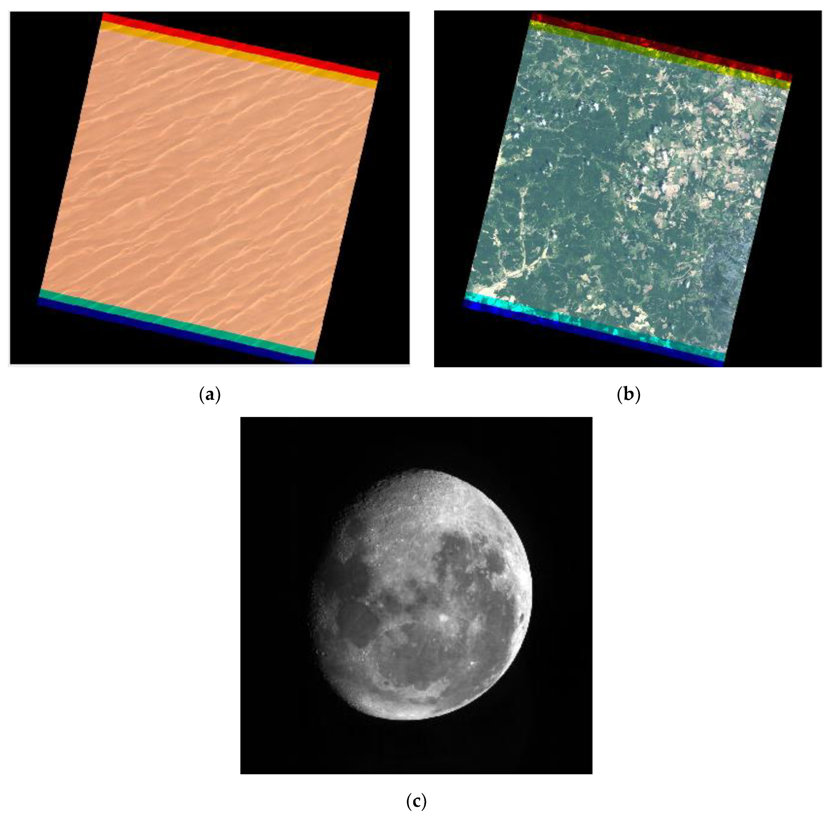
2.3.1. Radiometry

Radiometric Model

For all the spectral band k, the relationship between the digital count X_k (coded on 12-bit) and the observed radiance L_k for each pixel i is given by the following radiometric model:

X_k(i) = G_k,r × g_k(i,L_k(i)) × A_k × L_k(i) + D_k(i),

(1)

where:

• G is the video gain associated to the register r;
• g is the equalization coefficient for the radiance L_k;
• A is the absolute radiometric calibration coefficient;
• D is the dark current.

During the whole lifetime of the satellite, radiometric activities are split into two different types. Calibration activities lead to the estimation of all parameters in the radiometric model, whereas other activities aim to assess some performances of the instrument such as the modulation transfer function (MTF) and signal to noise ratio (SNR).

Calibration: Methods and Results

The calibration activities include viewing parameters optimization, defective pixel identification, dark signal estimation, equalization and absolute calibration. The two first tasks were performed only during the commissioning phase [8] because no variations are expected. Hence, this article focuses on the monitoring of the dark signal, equalization and absolute calibration [9].

• Dark Signal

Every electronic detector measures a signal when it powers up without any incoming signal at the entrance of the instrument. This signal is called the dark signal. The first step of an accurate radiometric calibration is the estimation of this signal and its monitoring because it could evolve slightly with time.

The method to estimate this contribution is based on night acquisitions over ocean sites. The main hypothesis using these specific acquisitions is that L_k = 0; thus, X_k = D_k. After a computation of a mean line to remove the temporal noise, the dark coefficient can be determined on each pixel. These coefficients were set after the commissioning phase and monitored during the VM01 phase. The Figure 5 compares the computed coefficients on several acquisitions with the ones used by the operational processing chain. The operational coefficient is updated only when the deviation is significant.

Here, only two typical bands are presented, but the other spectral bands present similar trends. A slight increase can be observed between 0.01 and 0.1 DC (for the nosiest band B1) per year. These results led to one update during the routine VM01 phase, on 1 June 2019.

• Equalization

The next step after the correction of the dark signal is the equalization. It consists of rectifying the non-uniformity of each pixel. To compute these coefficients, acquisitions over desert sites or snow sites are used. Indeed, these specific acquisitions are considered uniform scenes. This assumption allows us to correct the relative variation response of each pixel by combining a lot of these acquisitions and after generating a mean line to minimize the temporal noise. The following figures (see Figure 6) represent some acquisitions used for equalization.

During the commissioning phase, in addition to the usual equalization coefficients, radiometric spikes were observed and corrected [8]. These spikes are composed of two columns brighter than the adjacent background and two columns darker than the background. The sequencing of these four columns is reversed if the spike is located in the left register or in the right register. Their amplitude range is from 1 to 10 digital count, and it depends on the viewing parameters, whereas their location is stable in time. This phenomenon cannot be modeled as an additive nor as a multiplicative factor, so a new specific model had to be defined to correct these spikes. An example of the equalization effect is given in the Figure 7.

• Absolute Calibration

The final parameter of the radiometric model is the absolute calibration coefficient. These coefficients were determined during the commissioning phase, but they can strongly evolve all along the satellite lifetime. It is therefore important to accurately monitor the evolution of this coefficient for every spectral band. Several methods (see examples in Figure 8) are used to estimate and monitor the VENμS absolute calibration:

• cross-calibration with other sensors such as MERIS or Sentinel-2 with acquisitions over desert sites [10];
• cross-calibration with Sentinel-2 using Simultaneous Nadir Observations (SNO) [8,9];
• absolute calibration and temporal monitoring thanks to Moon images [9,11];
• absolute calibration with instrumented sites (Gobabeb in Namibia) [12];
• absolute calibration based on the Rayleigh scattering and ocean acquisitions [13].

Figure 8. (a) RGB image over the desert site Arabia 1; (b) RGB image over the SNO site in Kentucky; (c) Moon image.

Figure 8. (a) RGB image over the desert site Arabia 1; (b) RGB image over the SNO site in Kentucky; (c) Moon image.

The aim of every method is to compare VENμS satellite measurements with a reference given by another satellite in the case of cross-calibration or by a model and a field instrument for the absolute calibration methods. Due to programming concern, only the first three methods are still processed in the routine mode.

The approach chosen for updating these coefficients is to keep those set at the end of the commissioning phase and adjust them with the time difference estimated using the Moon method (see Figure 9). Afterwards, the slope correction can be checked by comparing the results obtained with the SNO and the desert methods.

An accurate monitoring of the temporal deviation of the absolute calibration coefficient can be conducted with Moon acquisitions. The same tendency as those shown in the previous figures is observed on all spectral bands, even if the spectral band B2 is more stable than the others. The measured temporal deviation is about 1% per year. These outcomes led to five updates (every 6 months) after the commissioning phase of VM01. The associated dates are 1 July 2018, 1 January 2019, 1 July 2019, 1 January 2020 and 1 July 2020. A validation of this slope correction was performed by comparing the results obtained with the two other methods using desert and SNO sites.

The figure (Figure 10) illustrates the good consistency between all the different methods. The calibration results are within the 5% specification and within the 3% goal specification for most of the bands. Nevertheless, some points are outside the requirements or have important error bars. There are several reasons for this. Firstly, B1 is the spectral band most impacted by the stray light and the Moon method is highly sensitive to that effect. Furthermore, B12 is a water vapor absorption band; therefore, the results on method using on ground targets (desert and SNO) are deteriorated. In addition, the VENμS spectral bands B5 and B6 do not have an exact associated Sentinel2 spectral band. The spectral interpolation step in the SNO method may generate inaccuracy, depending on the ground reflectance spectrum.

In conclusion, the VENμS calibration was well monitored and was updated all along the VM01 phase to compensate for the temporal deviation of each parameter in the radiometric model. The absolute calibration performance reaches the requirements for the entire VM01 archive.

Performances: Methods and Results

Even if the satellite is well calibrated after all the previous activities, several instrument performances need to be assessed to ensure the good quality of the products. Some instrument features cannot be improved by calibration activities due to the camera design. However, it is crucial to check and monitor these performances over time to detect instrument deterioration during the launch phase or during its lifetime in orbit. These activities include stray light and polarization correction estimations, modulation transfer function (MTF), signal to noise ratio (SNR) and fixed pattern noise (FPN) assessments [14]. Only SNR and FPN evaluations were monitored during the VM01 phase; therefore, this article focuses on these activities.

The stray light correction is not described precisely in this article, but it is crucial to highlight this point because stray light was one of the most important issues regarding VENμS. During ground test campaigns, two types of stray light were observed: the local ghosts for the type 1 and the cross-talk ghosts for the type 2. The first type is caused by the scattering of surfaces of the instrument and multiple reflections on detectors, filters or lenses and generates a large blurring effect. Cross-talk ghosts are caused by reflections of light from a band to another band and it generates a blurring replication of the landscape. Filters were developed to correct these artifacts [15].

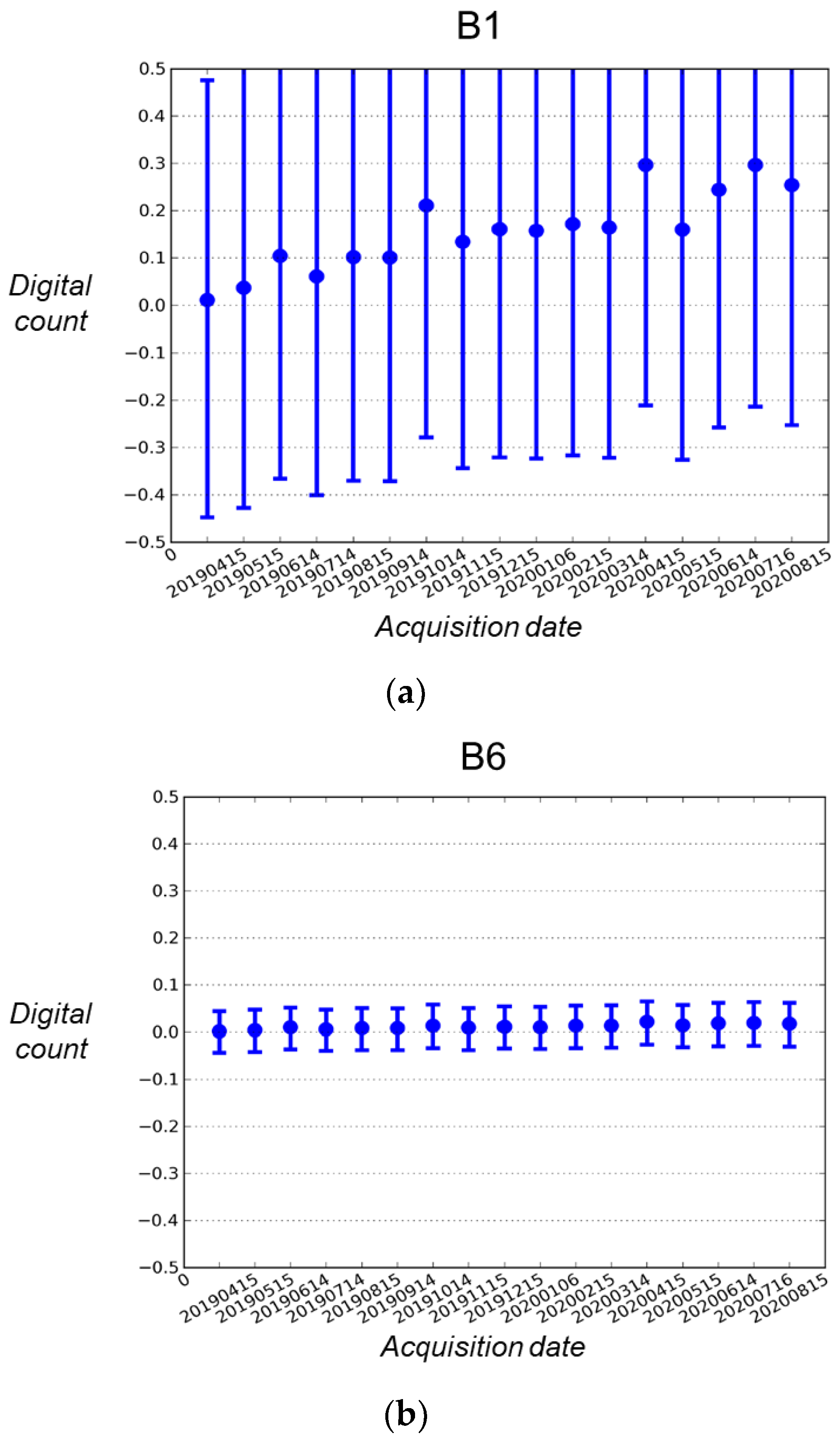
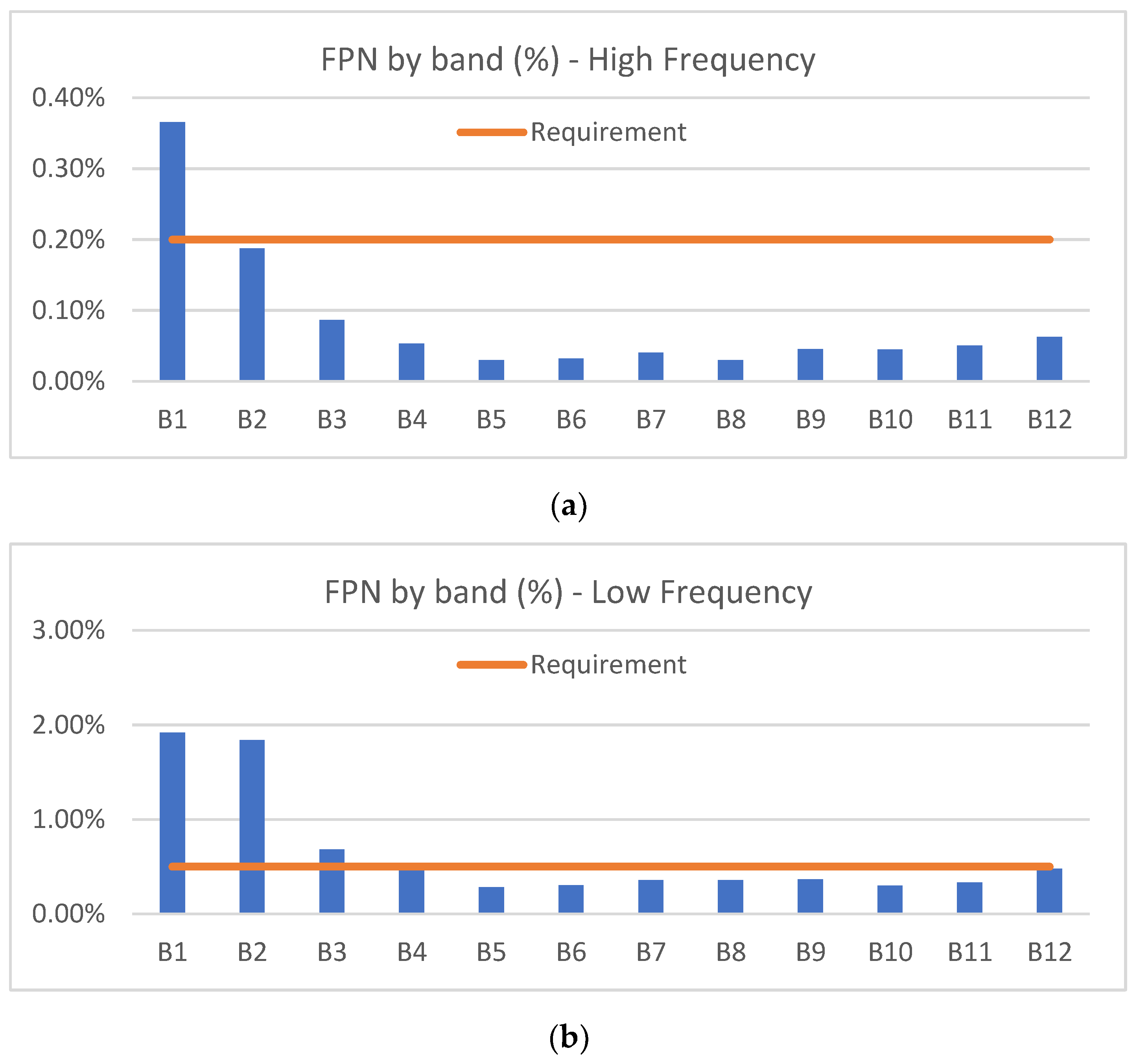
• Fixed Pattern Noise (FPN)

The equalization is an important step in the calibration processing. Once the equalization coefficients are computed, it is necessary to check their validity before their implementation into the production processing chain. As VENμS is a push-broom instrument, the expected artefact residuals are vertical lines directly printed in the images.

To assess the FPN, a method similar to the one used for the equalization step is conducted. The hypothesis of using a uniform landscape is also applicable and the specified used sites are the same. The main distinction between those two methods is the necessity to select different products for the estimation of equalization coefficients and for the assessment of the FPN. This allows us to validate the equalization coefficients on various dates and radiances to detect, among others, non-linearity issues and to determine when an equalization coefficient update is needed.

Two requirements are defined for the assessment of the high frequency and the low-frequency FPN. On the one hand, high frequency FPN is the difference between the response of any pixel and the average response over a 40-column sliding window containing that pixel. One the other hand, low frequency FPN is the difference between the average response over any 40-column sliding window and the average response over all active pixels. The two next graphs in the Figure 11 present the results of the FPN estimation during the last year of the VM01 phase.

As expected, after the commissioning phase, the requirements are not fulfilled for several spectral bands for both high frequency and low frequency FPN. Indeed, because of the radiometric spikes residuals and an accepted non-compliance concerning the non-linearity for the blue bands, it is arduous to reach the requirements for some spectral bands. However, the FPN computed with in-flight acquisitions is an overestimation of the actual FPN. In fact, even if the study areas in images are selected for their uniformity, the presence of the landscape generates a noise which is not due to the instrument equalization. This monitoring of FPN led to one update during the VM01 phase with the associated date 1 June 2019.

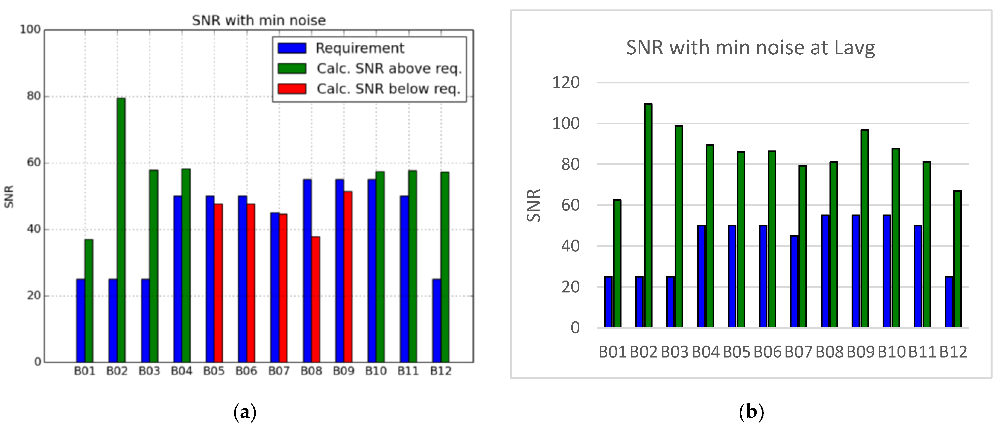
• Signal to Noise Ratio (SNR)

The SNR is directly derived from the instrument design. After the launch, it is difficult to increase this characteristic, but it is essential to monitor the SNR to detect potential issues or check the instrumental ageing. The FPN is a column noise, whereas the SNR is a line noise. Indeed, the SNR is a temporal noise which is given by the lines of a push-broom instrument such as VENμS.

The VENμS noise model, for a spectral band k, is given by the following equation:

$$Nois{e}_{\mathrm{k}}=\sqrt{a+b\times {\mathrm{L}}_{\mathrm{k}}}$$

(2)

where:

• $a$, $b$ are the coefficients of the model;
• $\mathrm{L}$ is the observed radiance.

The SNR estimation method is nearly the same as the one used to evaluate the FPN using uniform landscapes and assessing, this time, the line noise. As the noise model needs to be rebuilt with in-flight acquisitions to determine the coefficients a and b, it is essential to select numerous products to cover a wide range of radiance in order to improve the accuracy of the fit. Once the noise model is generated, the SNR can be computed for every radiance and compared with the requirements. The graphs below in the Figure 12 provide a comparison between the SNR computed on each spectral band and the requirements.

These diagrams show that, even if the results of some spectral bands are under the requirement for Lmin, which is the minimum specified radiance, for Lavg, the average radiance computed over all scientific sites, the SNR is highly satisfactory. It is highly challenging to generate an accurate noise model with in-flight acquisitions for the same reasons as for the FPN estimation method, which could hence explain these results.

Concerning radiometric performances assessment, every performance was evaluated during the commissioning phase and some of them were monitored all along the VM01 phase. Even if in some specific cases, in the worst cases in particular, the requirements were not reached, the overall VENμS radiometric performances entirely satisfy the scientists expectations and allow us to use VENμS products for numerous scientific applications.

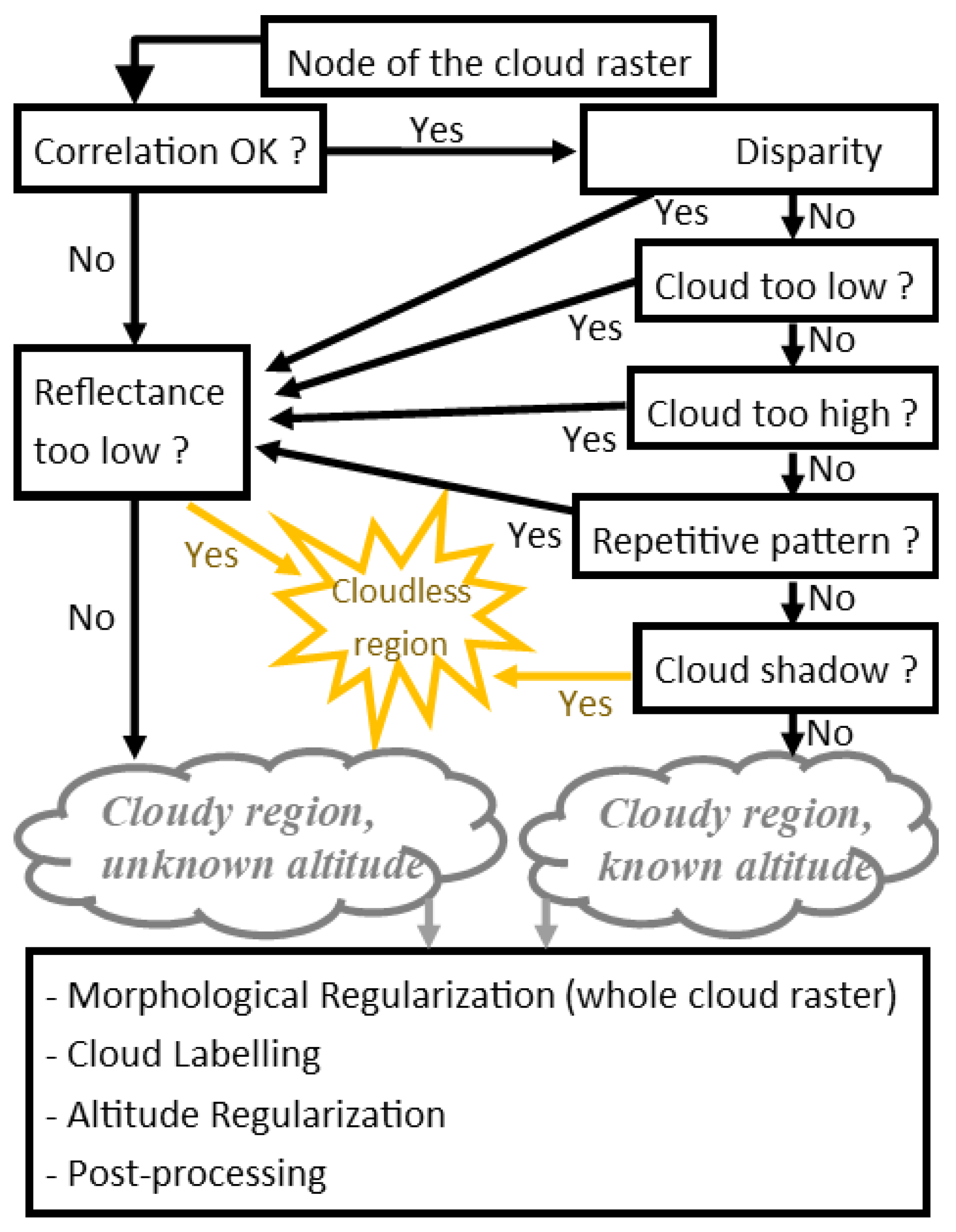
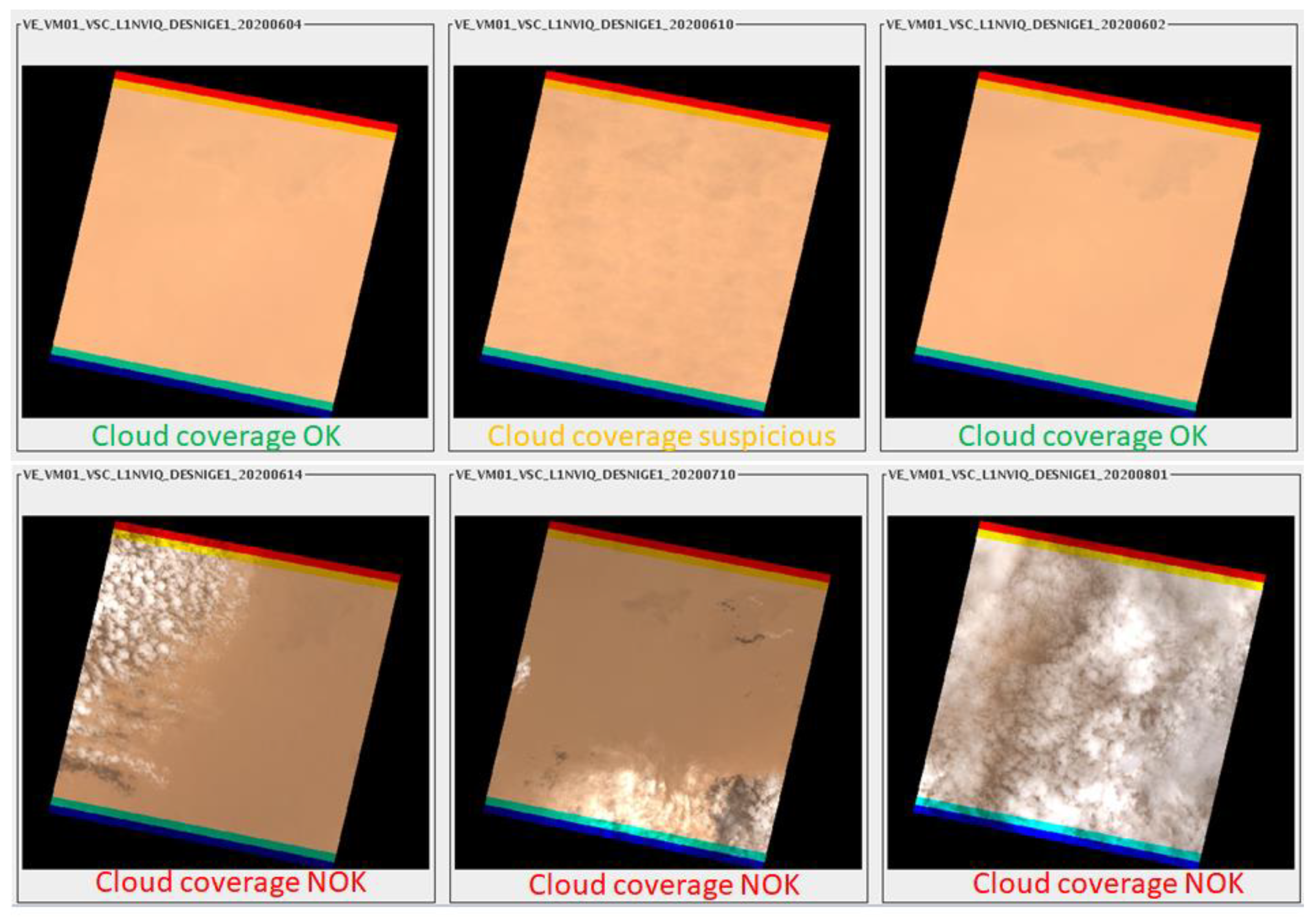
Cloud Mask Generation

One of the specificities of the VENμS satellite is the two stereoscopic bands B5 and B6. These two spectral bands have nearly the same spectral filter, as shown in the Figure 2, and the instrument focal plane design leads us to an observation angle difference of 1.5°and a temporal gap of 2.7 s between the acquisitions of these two spectral bands. During this time lag, clouds slightly move, and this movement can be observed directly in a single acquisition. These features allow us to detect clouds but also to estimate their altitudes. In general, cloud detection algorithms for Level-1 products are simply based on radiometric thresholds. Thus, this approach is quite innovative for an Earth observation satellite such as VENμS. The Figure 13 shows the decision tree of the cloud detection algorithm used for the VENμS Level-1 products.

This algorithm is based on the correlation of the B5 and B6 spectral bands. If the correlation works, it generates a disparity map which allows us to estimate the altitude of each pixel. Then, two filters were added to remove pixels with a too low or a too high altitude regarding an average cloud altitude. After these steps, a new filter was created to avoid false detections regarding repetitive patterns such as crop fields. In fact, correlations of repetitive patterns produce an unwanted disparity, and therefore, a false estimation of altitude regarding these pixels. The next step concerns the differentiation between cloud and cloud shadow, which can also be detected by the correlation. In the case where the correlation cannot be computed as expected, a radiometric step with reflectance comparison to thresholds is conducted to detect clouds even if their altitude cannot be estimated. The final stage of morphological regularization, cloud labelling and altitude regularization, is preformed to obtain a smooth final cloud mask. This raster, provided with the Level-1 VENμS products, provides the clouds position with a 5 m resolution, and the estimated altitude with a 50 m resolution, when the calculation is possible.

2.3.2. Geometry

Calibration: Methods and Results

During the commissioning phase, immediately after the VENμS launch, several geometric image quality activities took place in order to perform the geometric calibration of the instrument and the acquisition processing chain. They are described in a reference document [16]. Here, we present a summary of these activities.

The first geometric commissioning activity was to assess and correct the pointing bias in order to increase the steering performances.

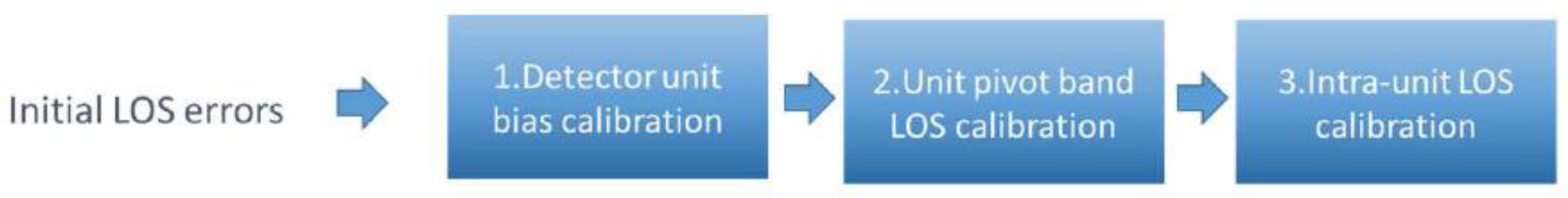
• Focal Plane Calibration

Then, focal plane calibration was performed to re-estimate the line of sight (LOS) of each pixel of each band, in order to fulfill inter-band and multi-temporal registration requirements. This activity is achieved by first calibrating the LOS of one band (B07 in our case) regarding an external reference (the Sentinel-2 Ground Reference Image—GRI): it is called the absolute focal plane calibration. After absolute calibration, a qualification was performed and residuals were estimated to about 0.1 pixel @2σ.

Afterwards, a relative focal plane calibration was performed in order to correct the LOS for all the other bands (except B07, which is the pivot band), thanks to dense tie point matching. The separation of the attitude and LOS errors contributions is a prerequisite to high quality calibration. However, by analyzing inter-band registration, attitude restitution errors were identified with registration errors that do not have a zero-mean value over acquisition time. The next illustration in the Figure 14 shows registration errors between B06 and B05 bands for several products. This leads to a bias in across-track direction, which complicates relative focal plane cartography.

A new strategy of calibration was set up in order to jointly estimate attitude and LOS errors using global optimization on several images (see Figure 15). This calibration was performed in three steps. The first step comprises correcting the LOS bias on unit pivot bands: B05, B06 and B10 with respect to B07. Then, the LOS of these pivot bands was calibrated at pixel level. Finally, the LOS calibration of other bands in the same detector unit (intra-unit LOS calibration) was conducted.

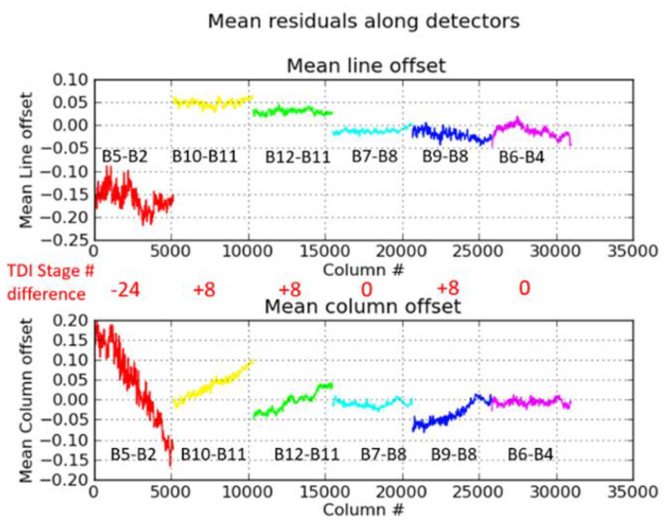
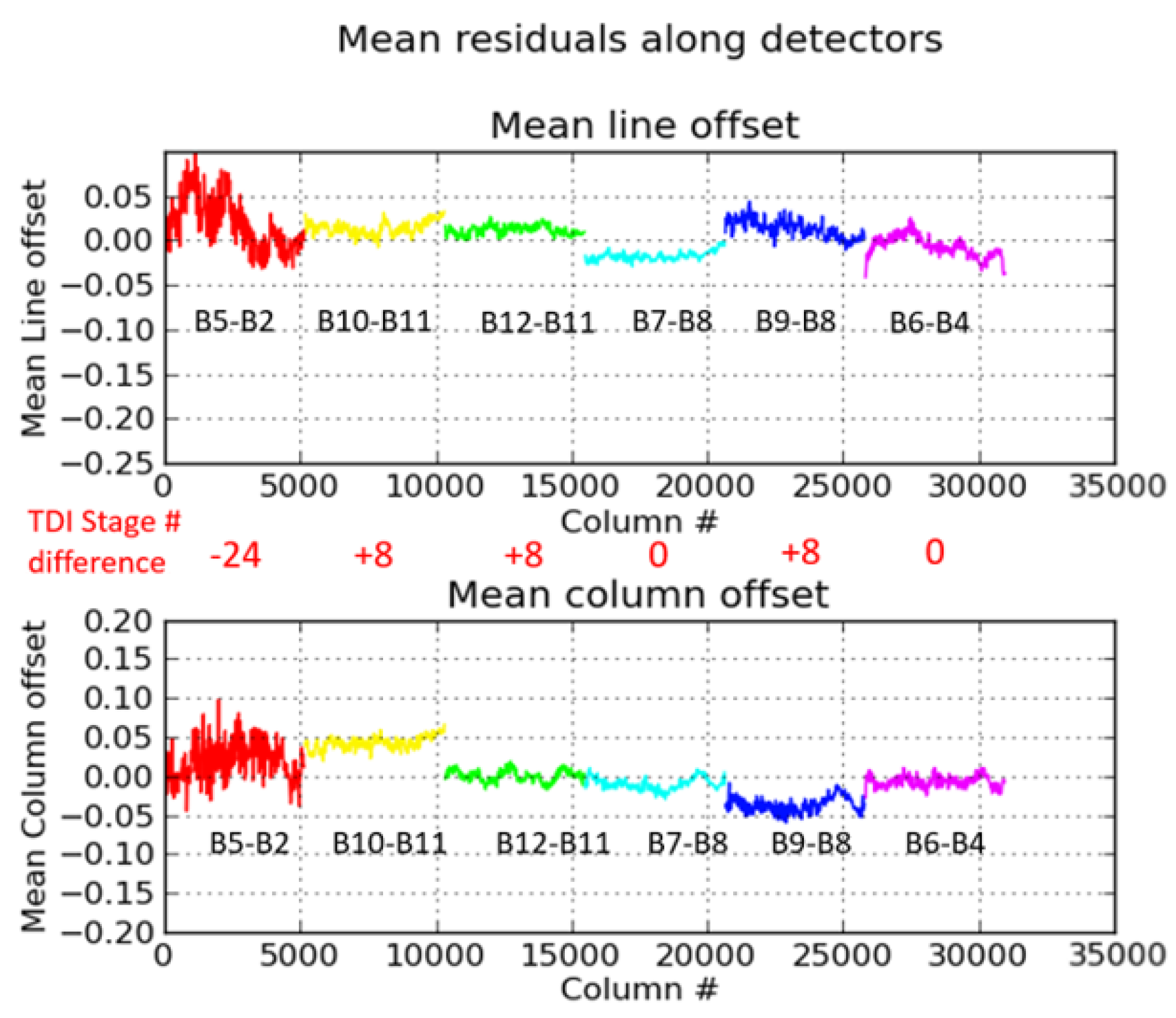
• TDI Mis-synchronization Calibration

An outcome of the VENμS in-orbit calibration is that time-delayed integration (TDI) optical sensors dedicated to push-broom satellite acquisitions can lead to geometric biases. These biases affect multiband registration accuracy if the considered bands are acquired with a different number of TDI stages; this also depends on the pitch angle. During in-orbit commissioning, the number of effective stages was adapted for each VENμS band to the Earth mean radiance in the considered spectral band. For instance, the B2 band is acquired using 32 stages of TDI to increase the signal to noise ratio, whereas B5 only uses 8 stages. For the extreme configuration of B2–B5 with, respectively, 32 and 8 stages, and for a 30° viewing pitch angle, projective mis-synchronization yields a differential magnification of 0.3 pixels (see Figure 16).

Nevertheless, these geometric biases were able to be analyzed and corrected thanks to a rigorous geometric modelling of the TDI stages. Mis-synchronizations were measured by the co-localization of a pixel belonging to the first stage with the stage N. The operation was repeated for regularly spaced pixels in the scene in order to assess field effects. Eventually, the correction was able to be integrated to the orthorectification process, biases being estimated for each image in the VENμS ground segment. As can be seen in Figure 17, the final registration performance assessment is far better: image magnifications were removed.

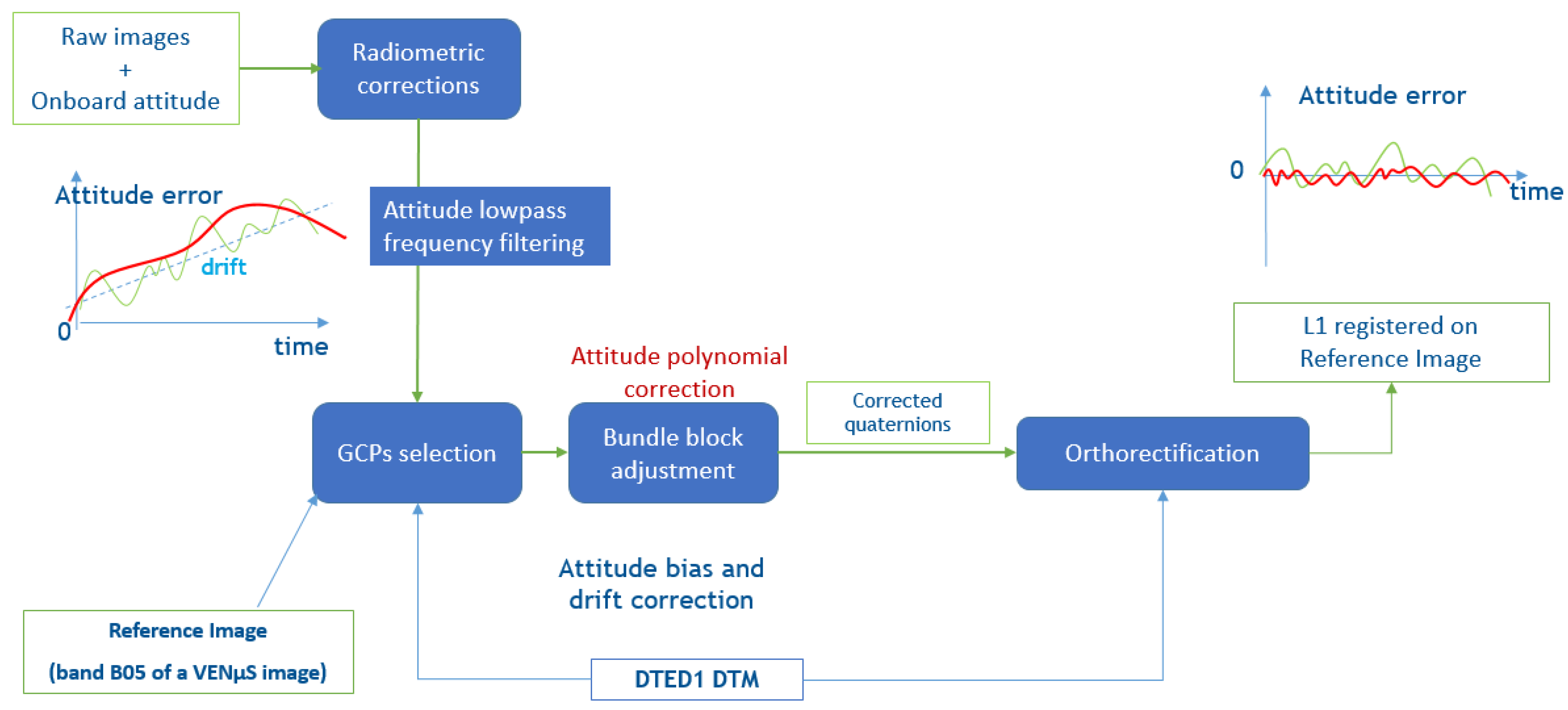
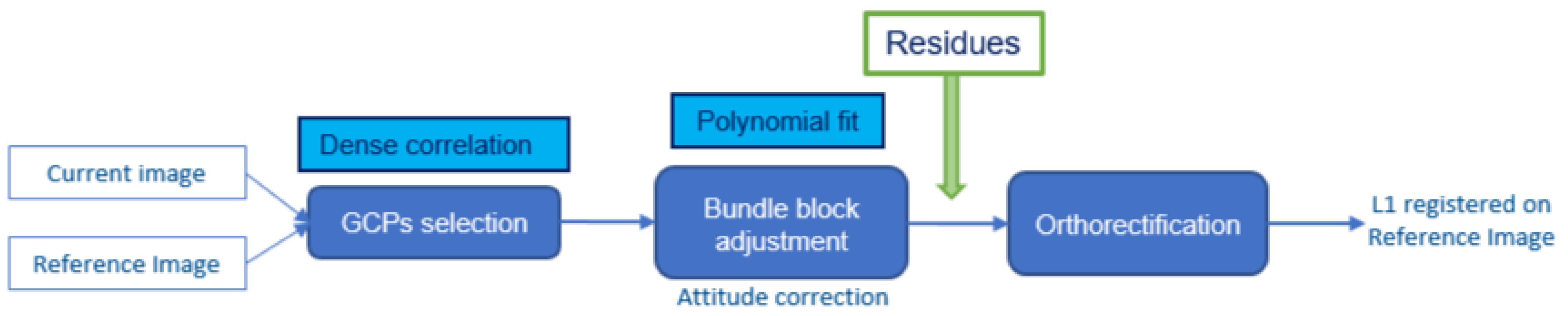
• Automatic Image Registration

After radiometric corrections in raw geometry, VENμS images were registered on a VENμS reference image defined by the following characteristics:

• a monospectral (B5 spectral band) VENμS Level-1A product;
• localization accuracy refined using a Sentinel-2 image specific to each site;
• processed from a cloudless acquisition.

In order to cope with attitude restitution errors, a first step of attitude low-pass filtering was added to L1 VENμS image processing as presented in the Figure 18. Tie points were then automatically computed between a VENμS image and its reference image. Using these tie points, the attitude was corrected by an adjustment of the parameters of the camera geometric model, using a polynomial correction. The attitude and LOS biases were jointly optimized in order to minimize the tie points location errors in a least squares reduction.

For this new attitude correction, dense ground control points (GCP) were needed. If the GCPs are not dense enough, due to cloud coverage or specific landscape such as water, the attitude polynomial correction will not be performed correctly. If a VENμS product is too cloudy, or if its landscapes are too different from the reference image, the correlation process fails. In the L1 processing chain, the resulting L1 product geometry is not corrected. This leads to an “invalid” L1 product, which is not distributed through THEIA portal.

As a consequence, this reference image and registration processing is very important for multi-temporal and multi-spectral registration performances.

Performances: Methods and Results

In this paragraph, the geometric performances of VM01 VENμS images are presented. These performances were computed using the products available at the end of VM01 mission (November 2020). A reprocessing of VENμS VM01 products is undergoing. The performances shall be improved after this reprocessing.

• Pointing Performances

To assess pointing performances, the acquisition center was computed from the useful image content. It was compared to the expected center as defined in the acquisition set definition (ASD) (see Figure 19). This monitoring was performed once a month on all sites from two consecutive cycles (~200 acquisitions). The results are presented in the Figure 20.

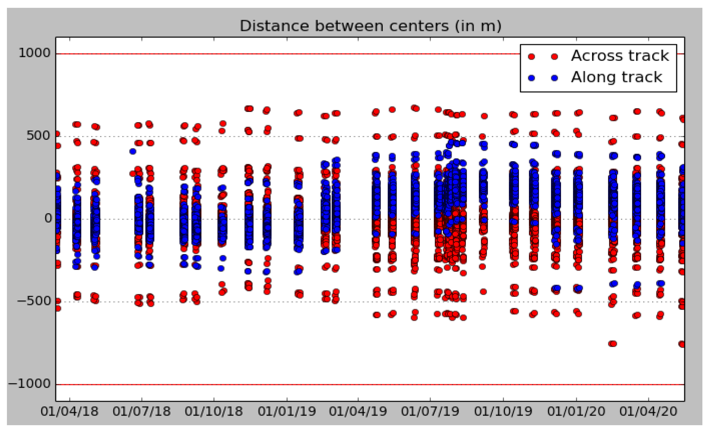
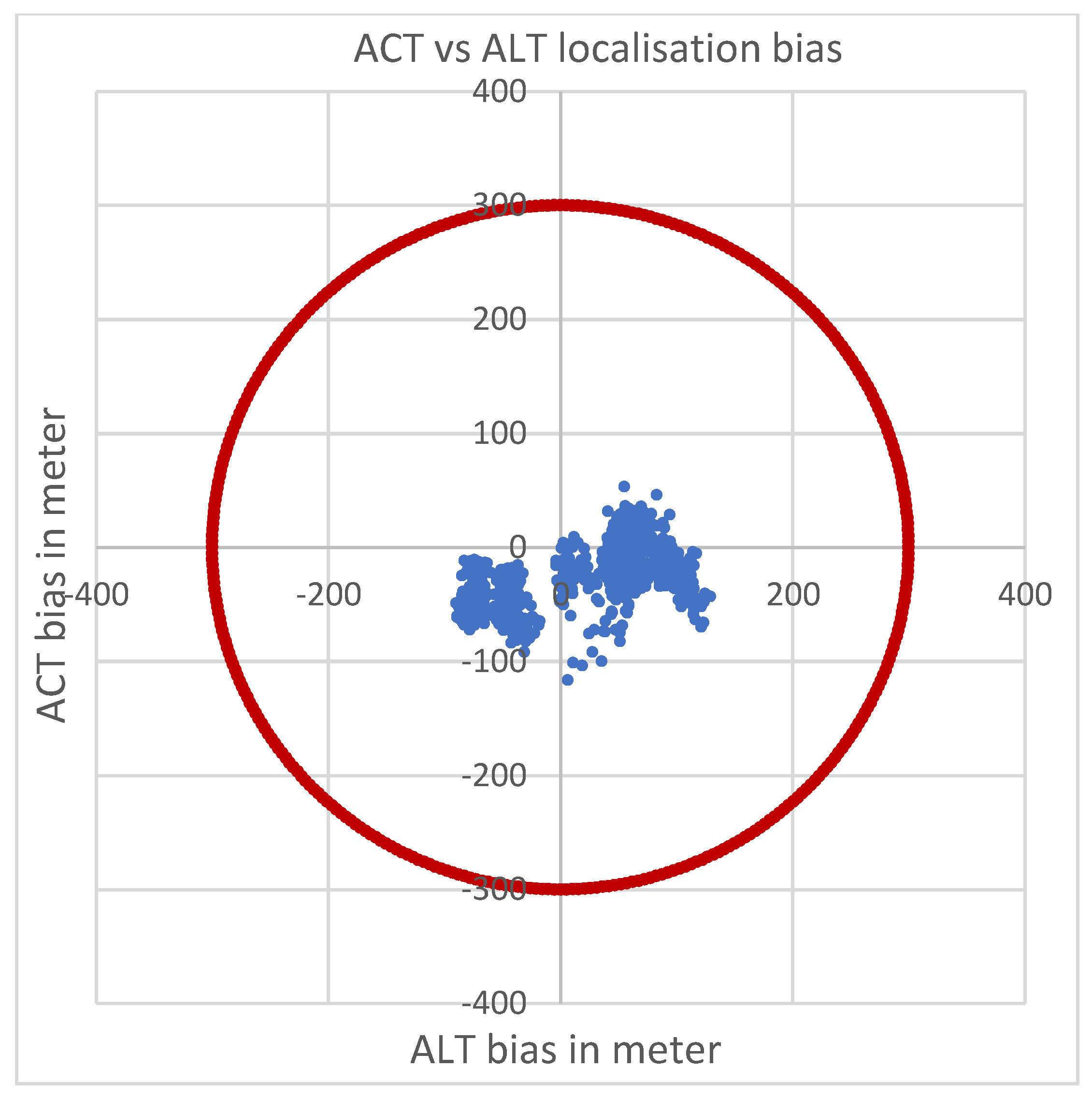
• Localization Performances

This performance corresponds to localization accuracy before refinement. It is assessed by computing the localization bias with respect to the VENμS reference image (see Figure 21). This performance was assessed on valid L1 products using ten specific sites which are characterized by good correlation and few clouds. These sites are spread around the world (North and South America, Australia, France and Israel).

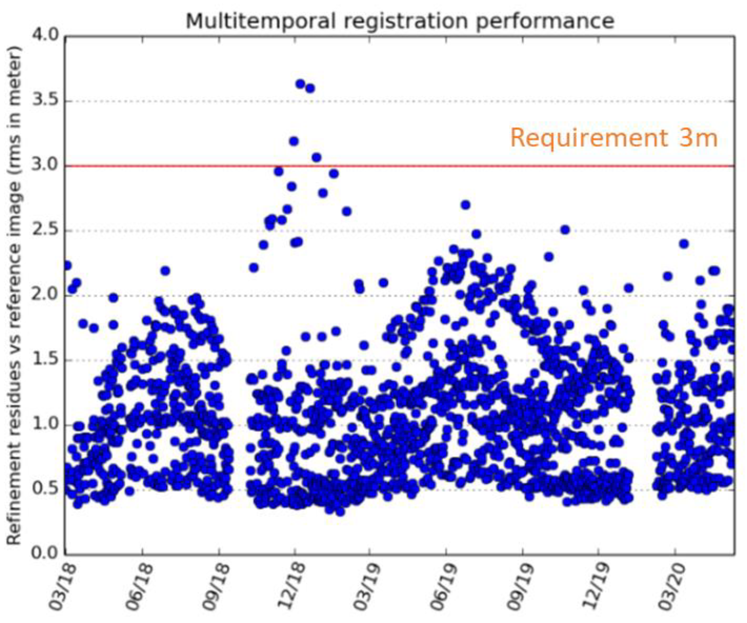
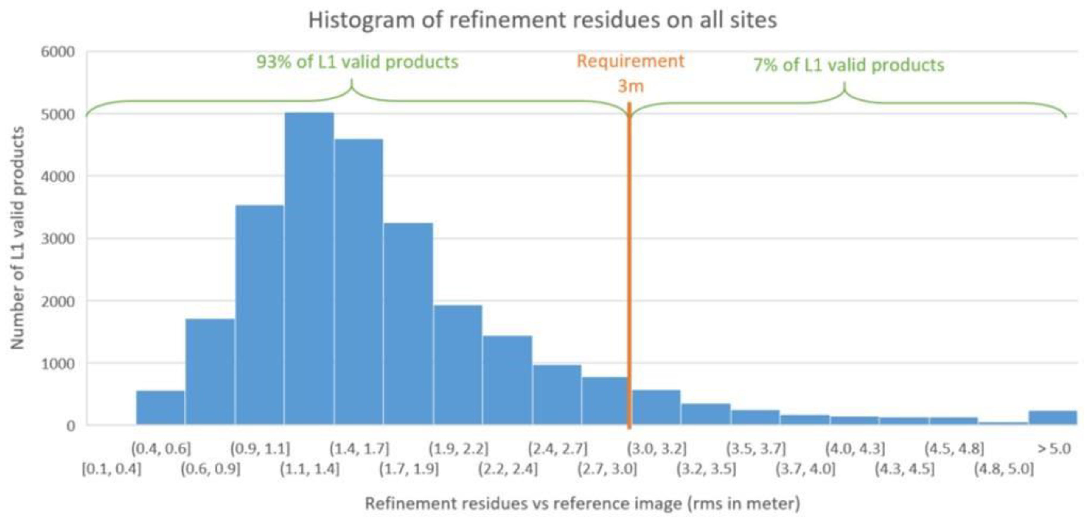
• Multi-Temporal Registration Performance

Multi-temporal registration performance was ensured by registration with respect to a reference image, using ground control points computation. The performance was evaluated directly using L1 processing chain by computing residues of ground control points after bundle block adjustment. The L1 geometric correction processing is shown in the Figure 22.

These residues, which contain the matching noise and the attitude residual errors, allow an easier follow up on all images as they are automatically computed during each L1 production. A geometric quality criterion was added to the header of each product.

The monitoring of multi-temporal registration was performed on eight specific sites with good correlation properties and few clouds. These sites are spread around the world (North and South America, Australia, France and Israel).

The Figure 23 shows that multi-temporal registration performances of VENμS products are stable. Some sites perform above the requirement, which is 3 m RMS. For instance, the long site SO1 is above the requirement, as there is less adequation between attitude and polynomial fit in the attitude correction processing. In addition, when there is less similarity with the reference image due to landscape changes, multi-temporal registration performance tends to decrease as there are fewer points in the correlation with the reference image. Therefore, correlation results were closely followed to change reference image when needed.

The Figure 24 gives the repartition of multi-temporal refinement residues on all sites. It allows us to see what is the proportion of sites that fulfill multi-temporal registration performance during VM01 phase.

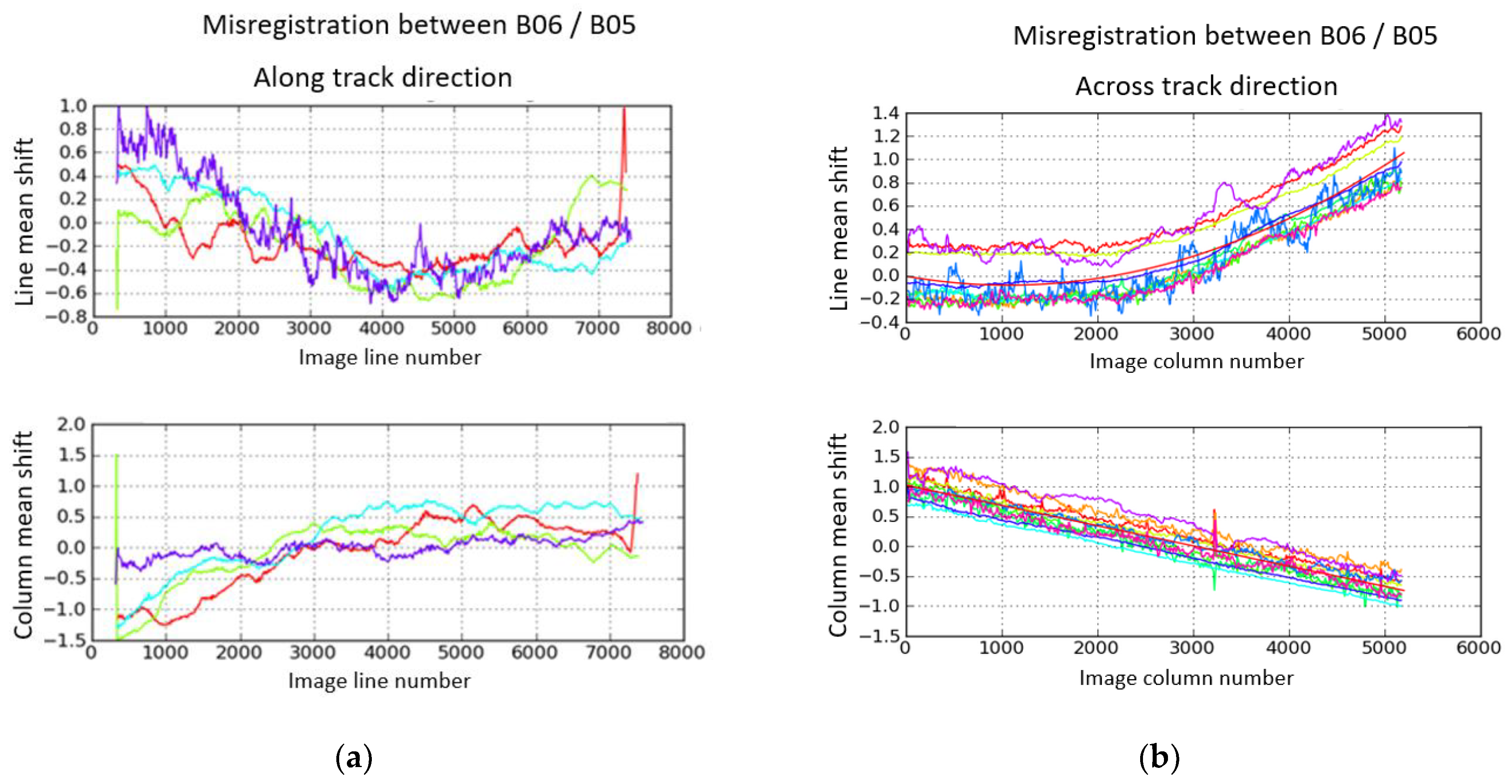
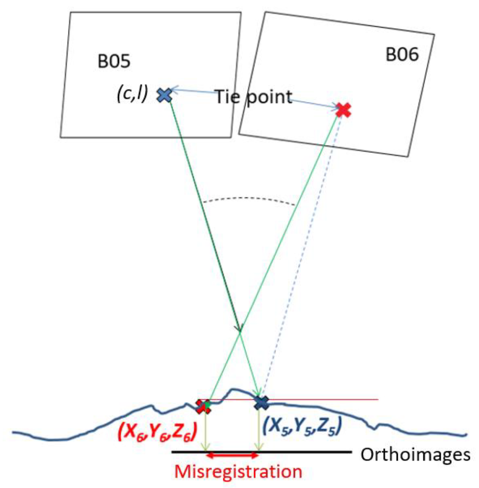
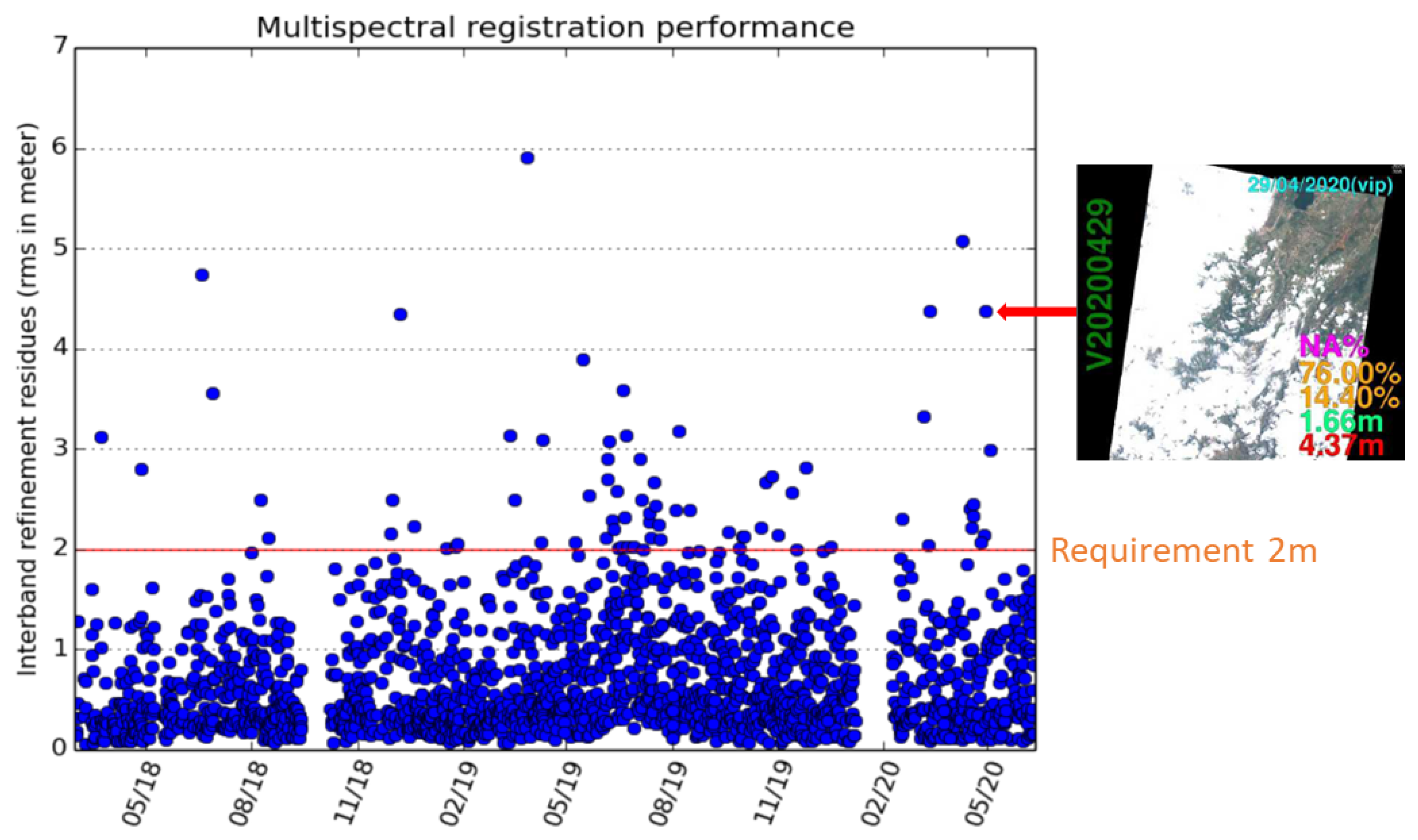
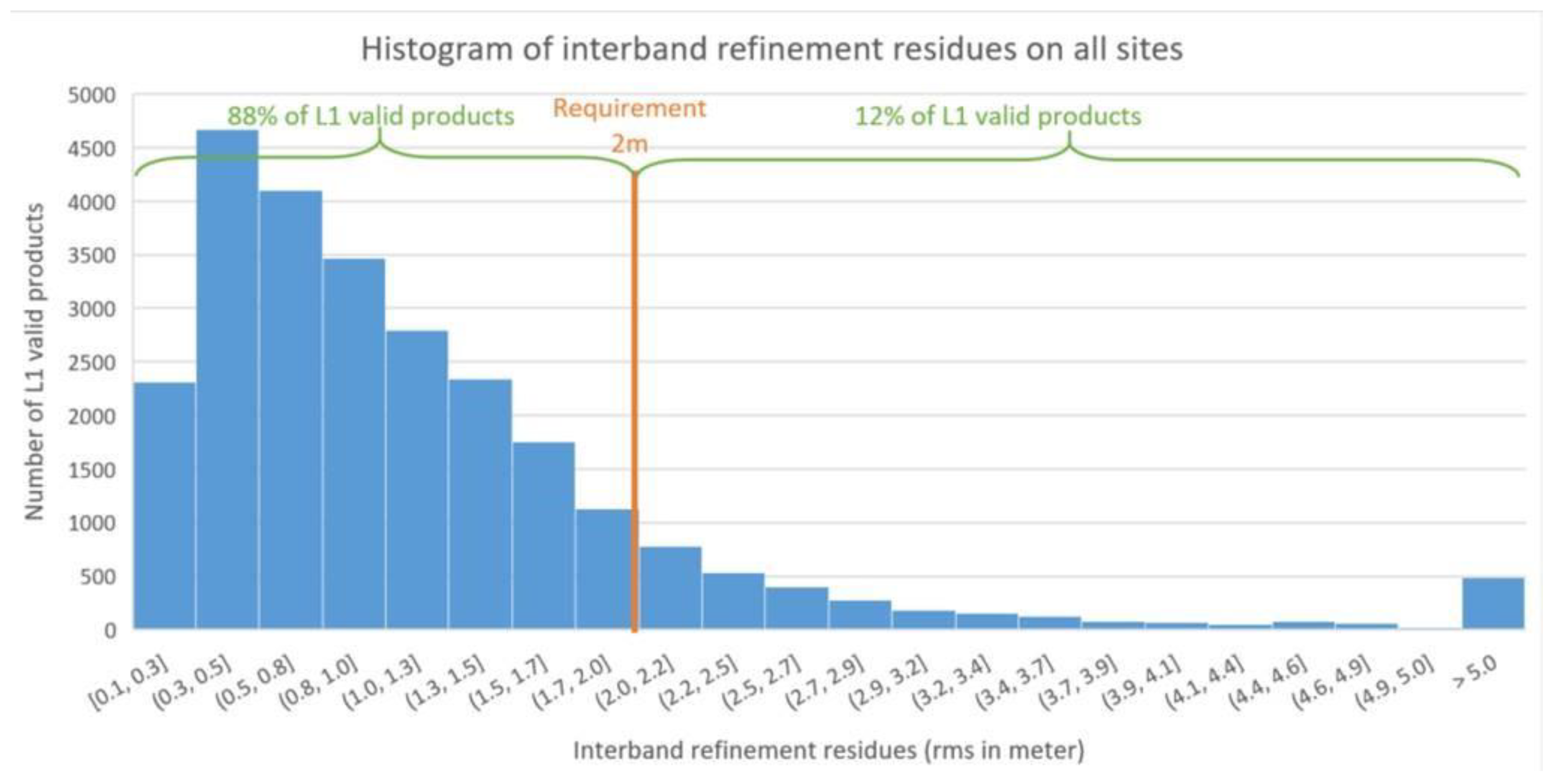
• Multi-Spectral Registration Performance

Multi-spectral registration performance is assessed by inter-band correlation using B05/B07, B05/B06 and B09/B10 band couples. The misregistration errors are computed automatically during each L1 production. This allows the easier monitoring of all images. A quality criterion was therefore added in all products. The computation principle is describe in Figure 25.

Monitoring was performed on eight specific sites with good correlation and few clouds. These sites are, as for the multi-temporal registration performance, spread around the world (North and South America, Australia and Israel).

The Figure 26 shows the multi-spectral registration performance results evaluated from inter-band registration residues.

The results show that the multi-spectral registration performances of VENμS products are stable. Some sites have a performance above the requirement, which is 2 m RMS. However, if we analyze these products, most of them were cloudy products, as shown in the example above. Some parts of the clouds were taken into account in the inter-band correlation process. In this case, the resulting residue misrepresents the real multi-spectral performance.

The Figure 27 provides the repartition of multi-spectral refinement residues on all sites. It allows us to see the proportion of sites that fulfill multi-spectral registration performance during the VM01 phase.

In conclusion, geometric image quality performance assessment shows a stability of all performances of VENμS products during the VM01 phase.

2.4. Performances of Level-2 VENμS Products

2.4.1. Level-2 Processing Method

The VENμS Level-2 processing performs atmospheric corrections which convert Level-1 top-of-atmosphere reflectances products into Level-2 surface reflectances. It produces surface reflectances for each band of VENμS, with masks of clouds, cloud shadows, snow, water and maps of retrieved aerosol optical depths and water vapor contents.

VENμS Level-2 processing is performed with MAJA atmospheric correction software, which is based on the Multi-temporal Atmospheric Correction and Cloud Screening Software (MACCS) [17] and includes some modules of ATCOR software [18], which is also used to generate SENTINEL-2 Level-2 products within the French THEIA land data center.

For clouds, cloud shadows masking and aerosol optical depths assessment, MAJA uses both multi-spectral and multi-temporal methods. Multi-temporal methods are based on the assumption that surface reflectances change slowly in time in comparison to cloud and aerosol contents.

MAJA methods are detailed in MAJA ATBD [19], but are summarized in the following steps:

• estimation of water vapor content using information from VENμS B12 band (909 nm) corresponding to a strong water vapor absorption band and B11 (861 nm) used as reference band outside the absorption band;
• correction of atmospheric gases, including water vapor; absorption with the Simplified Model for Atmospheric Correction (SMAC) software [20];
• determination of cloud, cloud shadow and water masks by combining multi-spectral and multi-temporal methods;
• determination of aerosol optical depths using both multi-spectral and multi-temporal methods;
• correction of aerosol absorption and scattering and Rayleigh scattering using look-up tables, precomputed with SOS (successive orders of scattering) radiative transfer code;
• adjacency effects corrections;
• slope and aspect corrections.

2.4.2. Level-2 Performances Assessment

The quality of water vapor contents and aerosol optical depth (AOD) determined by MAJA and used in the atmospheric inversion play a major role in the Level-2 surface reflectance quality.

In situ measures of AOD and water vapor are acquired daily by the worldwide photometer network AERONET [21] and provide good references to assess the quality of VM01 Level-2 water vapor and AOD estimations.

Water Vapor Content Quality

The next figure (see Figure 28) compares VM01 Level-2 products’ water vapor contents to those measured by AERONET. Each point corresponds to concomitant AERONET and VM01 VENμS measures. The measures with high confidence comparison criteria are drawn in blue (AERONET measurements are available at Level-2 and at least 80 percent of pixels in a 1 km region of interest around the photometer are unmasked), whereas those with medium confidence comparison criteria are drawn in red (AERONET measurements are Level-1.5 ones or the percentage of unmasked pixels in a 1 km region of interest around the photometers is between 40 and of 80 percent). Water vapor estimation shows goods performances. One can notice an overestimation of water vapor for high water vapor contents.

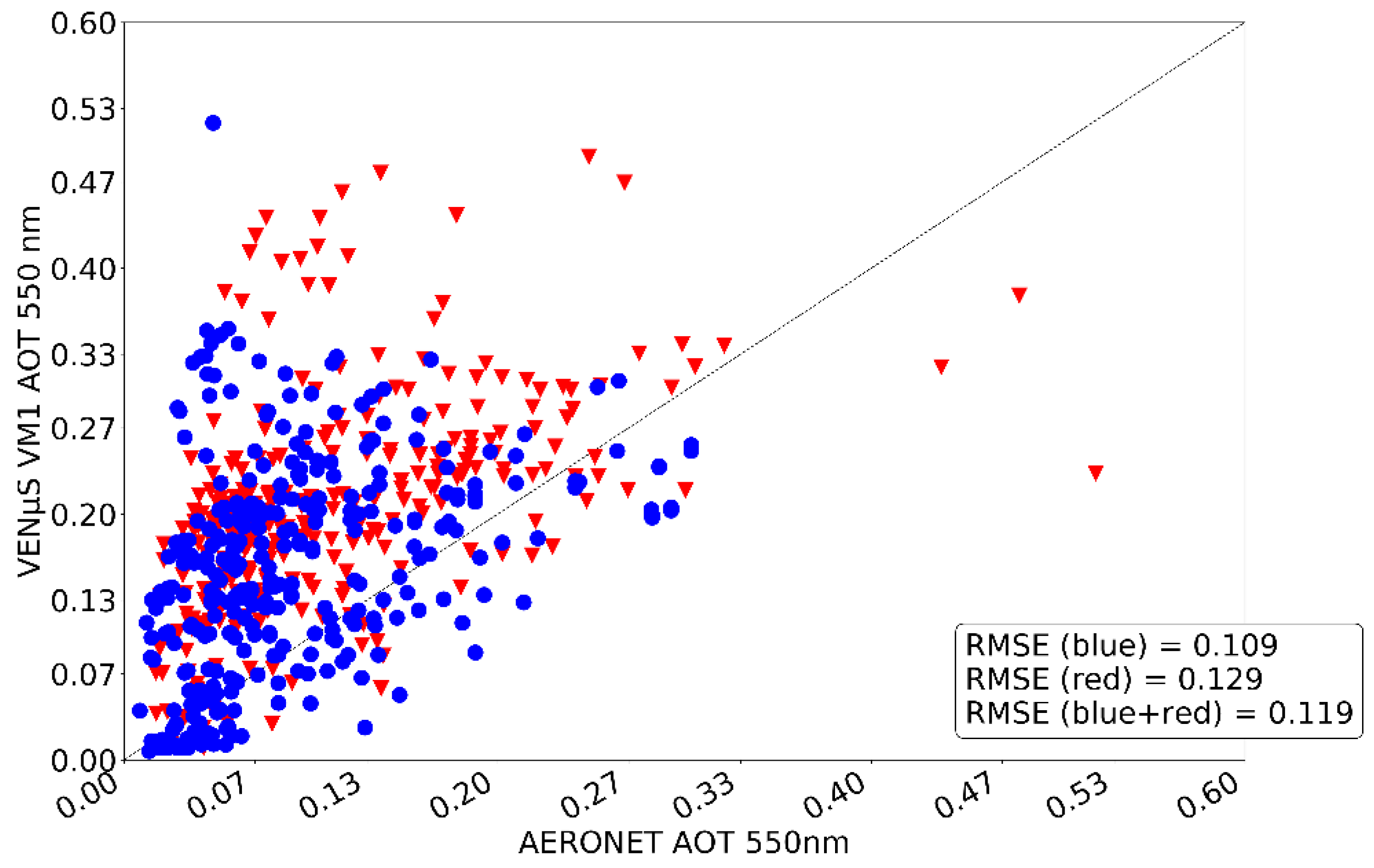
Aerosol Optical Depth Quality

The Figure 29 compares VM01 Level-2 products’ AOD at 550 nm to those measured by AERONET. Each point corresponds to concomitant AERONET and VM01 VENμS measures. The measures with high confidence comparison criteria are drawn in blue (AERONET measurements are Level-2 ones and at least 80 percent of pixels in a 10 km region of interest around the photometer are unmasked), whereas those with medium confidence comparison criteria are drawn in red (AERONET measurements are Level-1.5 ones or the percentage of unmasked pixels in a 10 km region of interest around the photometers is between 40 and of 80 percent).

AOD at 550 nm is overestimated. After investigation, this over-estimation was found to be due to the VENμS site (ARM) which was used to parametrize the AOD multi-spectral retrieval method, which has a particular spectral signature with red soils. Moreover, in cases of snow, the AOD can also be overestimated. Studies were conducted to improve AOD retrieval quality: a new parametrization of the AOD multi-spectral retrieval method was performed with a much wider range of VENμS images and a snow mask was implemented. These improvements, as well as the aerosol model estimation thanks to CAMS auxiliary data [22], will be considered in the coming VM01 product reprocessing.

2.5. Performances of Level-3 VENμS Products

2.5.1. Level-3 Processing Method

The weighted average synthesis processor (WASP) is used to produce periodic syntheses of surface reflectance. Its aim is to simplify the work of users, by providing almost cloud free images. Most Level-3A products are based on a best available pixel method [23], which selects, for each pixel, the best date in a surface reflectance time series. The most classical selection criterion comprises selecting the date for which a vegetation index is maximal [24], knowing that clouds have a very low vegetation index. This criterion has the advantage of discarding potentially undetected clouds. However, the drawback of all best available pixel methods is that two adjacent pixels may have been selected in two different dates, with different vegetation development stages, different view and solar angles, or different atmospheric correction errors. These differences result in the addition of a salt and pepper noise on the images.

To avoid this noise, an alternative consists of averaging all the cloud-free and shadow-free observations [25]. These methods require a very good detection of clouds and shadows, as every detection omission will result in including cloud or shadow reflectance in the average. As the quality of the detection of clouds by MAJA is very good [26,27], it is possible to apply such a method to VENμS. In the case of VENμS, with a revisit of two days and, given an average cloud cover of 70%, it is expected that every period of 20 days should provide more than three clear observations per pixel on average. We decided to provide Level-3 products on the 1st and 16th of each month. Each synthesis is based on 23 days of acquisition, using time windows starting 11 days before and ending 11 days after the synthesis date. Instead of a plain average, the WASP processor uses weighted averages for observations far from a cloud, with a low AOD, or close to the synthesis date. A complete description of the method is given in a document in reference [28].

2.5.2. Level-3 Performances

In the frame of the last operational processing, not all the Level-3 products were generated by THEIA. The Figure 30 illustrates the visual quality of the Level-3 processed by THEIA. By showing the same area, in four different Level-3 products, it is possible to monitor the evolution of landscapes with accuracy.

3. Operations

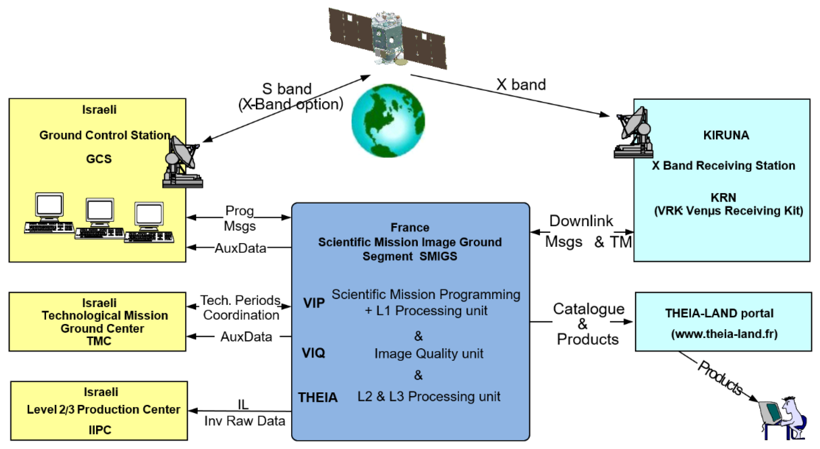
3.1. System Overview

The VENμS mission is ensured by several entities which can be seen in the next figure (Figure 31). In Israel, there are the Ground Center Station (GCS) and the Technological Mission Ground Center (TMC), which operate the satellite and analyze technological telemetry. There is also the Israeli Level-2 and -3 Production Center (IIPC). The Scientific Mission Image Ground Segment (SMIGS) is located in France, and includes the L1 processing unit (VIP), the L2/L3 production unit (THEIA), the scientific mission programming unit (VIP), the products catalog and portal (THEIA-LAND) and the image quality center (VIQ). Finally, the Kiruna Receiving Station (KRN) is in Sweden.

The list of the functional interfaces, related to system operations, are introduced below:

• SMIGS and TMC exchange coordination information and files for scheduling scientific mission and technological mission period;
• SMIGS and GCS coordinate themselves to implement scientific mission, and elaborate downlink plans for X-Band Ground;
• TMC and GCS plan technological mission implementation, and exchange information on spacecraft state and satellite telemetry reports;
• GCS and Spacecraft exchange commands and telemetry;
• GCS and KRN station exchange orbital elements;
• Spacecraft and VENμS Receiving Station have Payload telemetry as main interface;
• SMIGS and VENμS Receiving Station exchange payload telemetry downloaded;
• TMC and VENμS Receiving Station exchange auxiliary data downloaded (as well as GCS and VENμS Receiving station);
• SMIGS and IIPC: periodically, the raw inventoried data and the L1 products relevant to Israel, when updated at CNES: ground image processing parameters (GIPPs) for L2 and L3 processes.

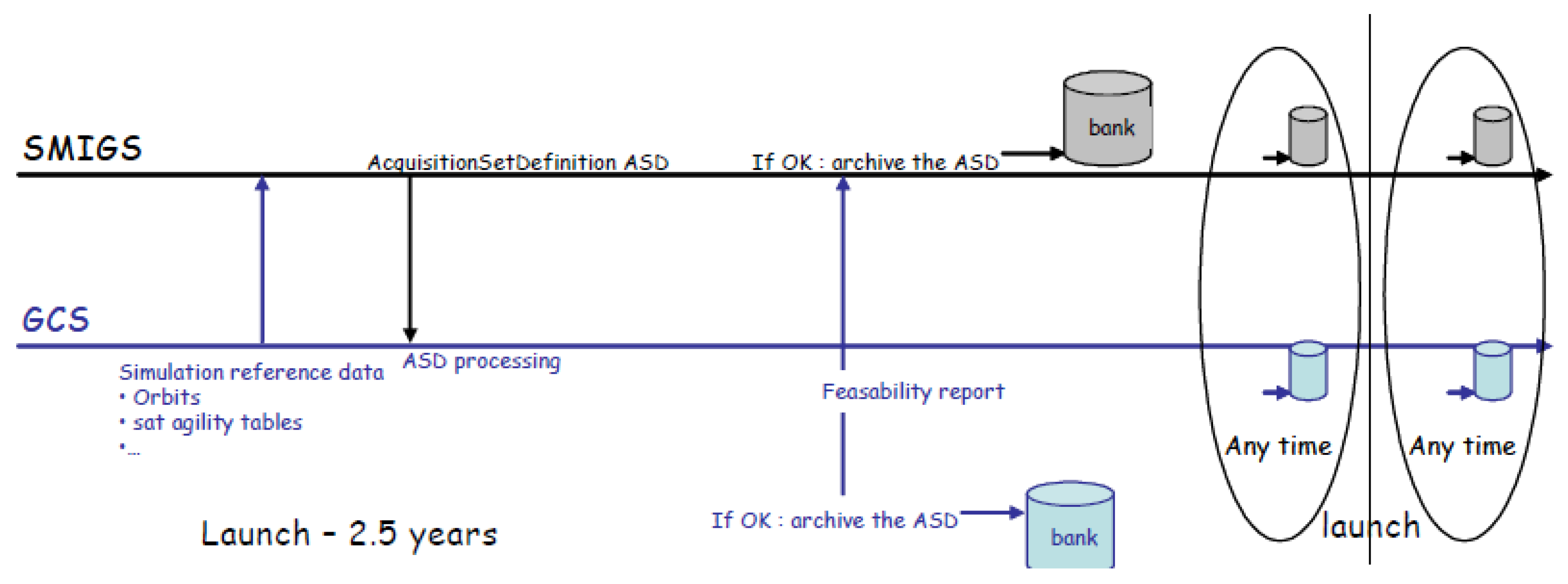
3.2. Mission Programming

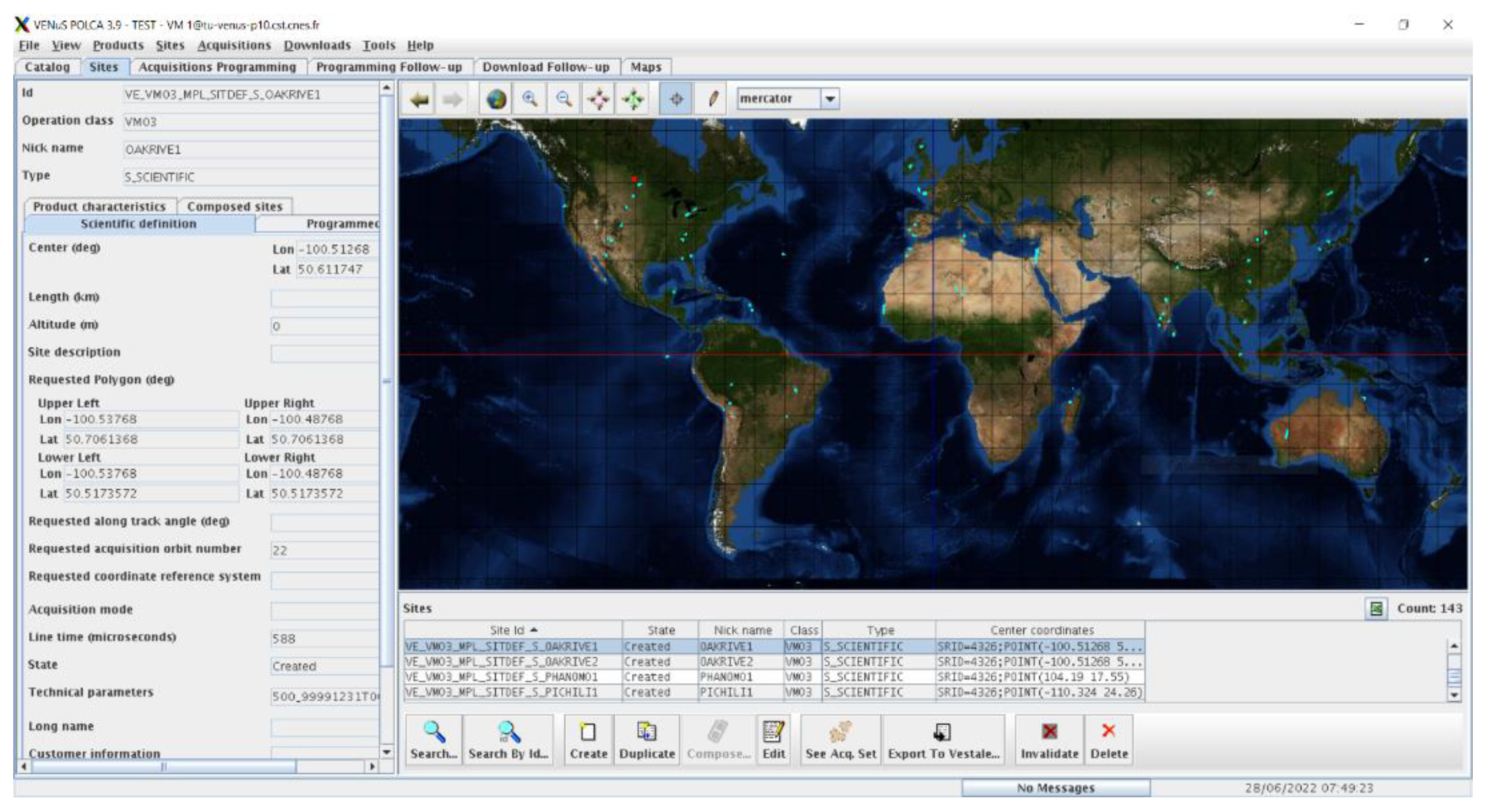
3.2.1. Acquisition Set Definition

The scientific programming for the VENμS mission was established from requests of scientists, for Earth observation studies, and from CNES image quality experts, for instrument calibrations, specifically geometric and radiometric ones. These requests were made during the call for proposals. The proposals on Israeli territory were selected by the principal investigator from the Ben Gurion University (Israel), while proposals on other territories were selected by the principal investigator from the CESBIO laboratory, at Toulouse (France).

Once the sites selection was closed, it was necessary to verify the feasibility of acquiring the areas chosen, in order to create the set of sites that were to be acquired during the mission. This activity is the responsibility of the SMIGS VIP team. The first step is to configure the scientific sites in a specific VIP tool, named POLCA for ‘Programming On Line And Catalog’ in order to generate an acquisition set definition reference (ASD). The characteristics of each site, such as its type (calibration or scientific site), the coordinates of its polygon, the length of the acquisition and the acquisition angles, were entered by VIP operators on POLCA GUI, as presented in the Figure 32.

To perform the best configuration in the system, various types of sites can be defined:

• a scientific site: a piece of earth of one to two contiguous images in given view angle positions;
• a composite site: a piece of earth of more than two contiguous images in given view angle positions;
• a calibration site: a piece of the planet continuously imaged in given view angle positions for image quality monitoring;
• a calibration/scan/strip: a piece of the planet continuously imaged in given view angle conditions, that corresponds on board to a time slot where the camera video output is continuously recorded;

For a second time, these sites were exported in another VIP tool named VESTALE for ‘VENμS Simulation Tool for Acquisition and download plan Elaboration’. This tool simulates the site acquisitions conducted by the satellite and allows us to confirm or not confirm compliance with some mission constraints, such as the onboard memory allocations and prohibition zones. In cases of conflicts, alerts are shown on the GUI, leaving to the operators the choice of action in deciding how to solve the conflict. Usually, the solutions are to remove the site that cannot be acquired, or to change the acquisition angle, as is the case in the examples below (see Figure 33).

Once the ASD is validated by the VIP at SMIGS, the last step is to check the acquisition set definition (ASD) is compliant with the whole mission constraints, considering the satellite resources that only Ground Control Segment (GCS) knows. To do this, the ASD is provided by the VIP to the GCS in order to confirm its operational feasibility, assuming a nominal orbit. If any conflict is identified, GCS notifies VIP team who is in charge of re-exercising the ASD according to GCS alerts. However, if the ASD is compliant with all constraints, it is checked out and tagged as valid by GCS. Then, it can be operated in the VIP center.

It is possible to have many valid ASDs in the VIP center. Nevertheless, only one can be activated in a defined period. The ASD repository allows operators to activate a specific one according to mission needs, such as seasonal effects, for example.

Finally, to prepare an operational scientific programming, VIP operators activate an ASD in the POLCA tool. Then, a request is sent to GCS, who accepts the set of acquisitions and considers it in its programming plans. The Figure 34 provides an overview of the scientific mission process.

During the 2.5 years of the VM01 mission, about 15 ASDs were programmed: some sites footprints have been changed, while others have been removed or added. On average, a VM01 ASD contained between 108 to 126 acquisitions that represents between 157 and 189 scientific sites (see Figure 35).

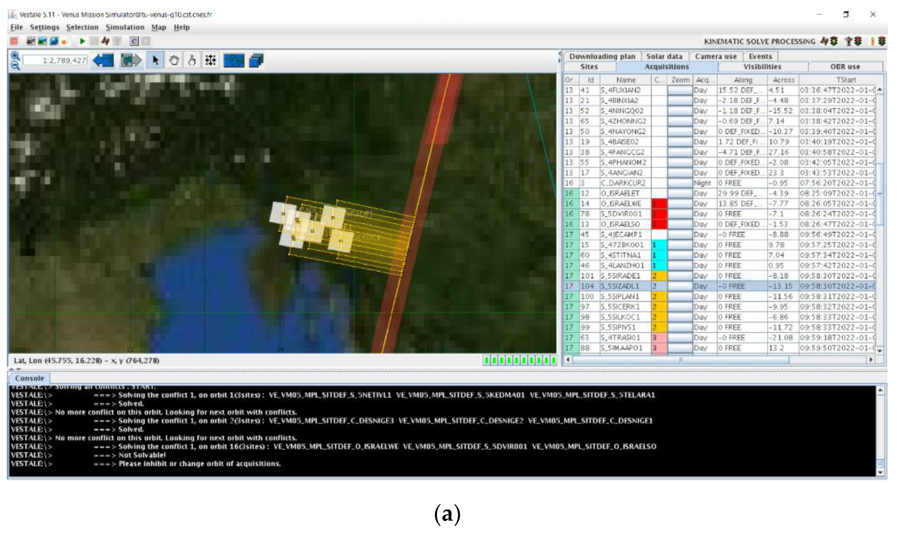
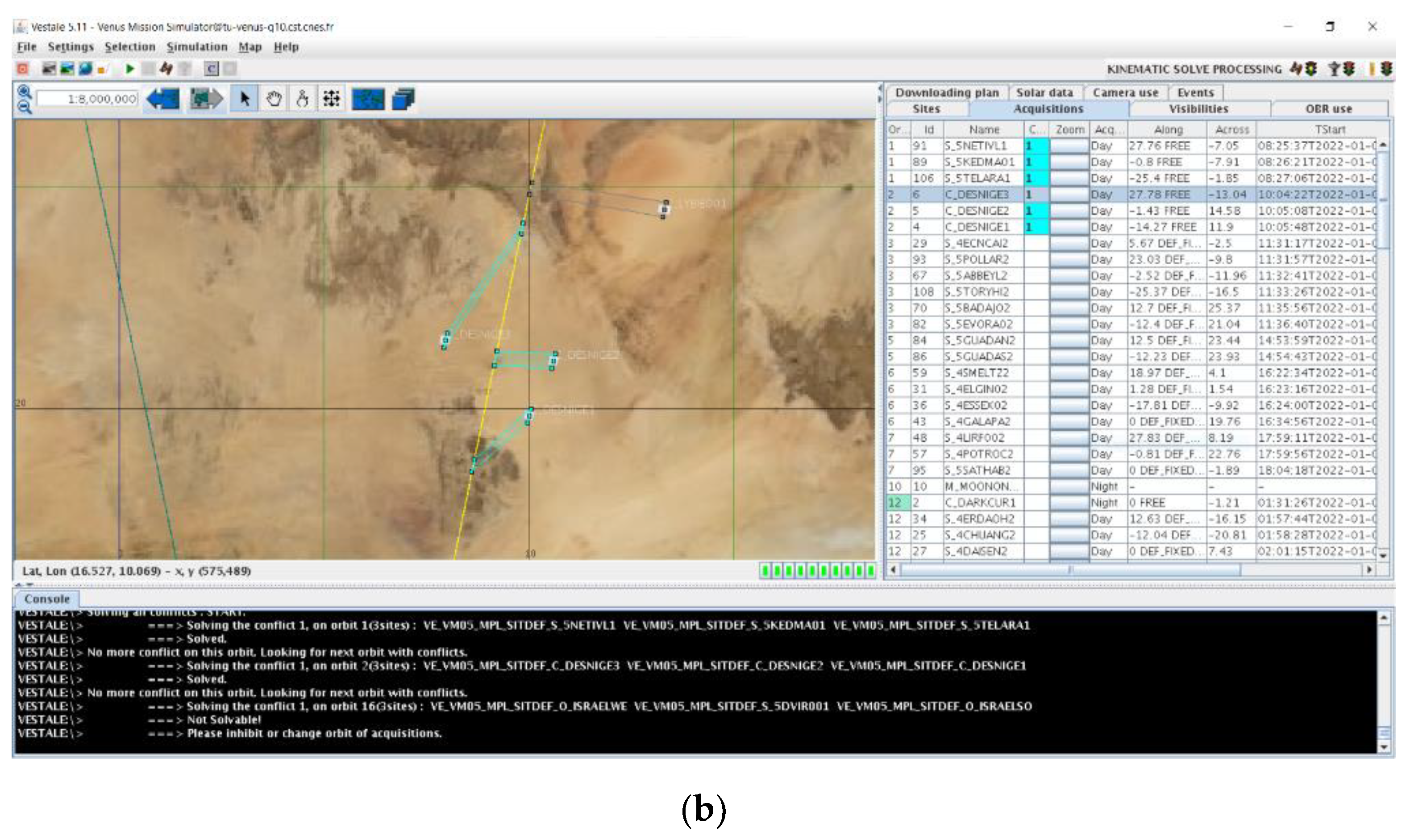
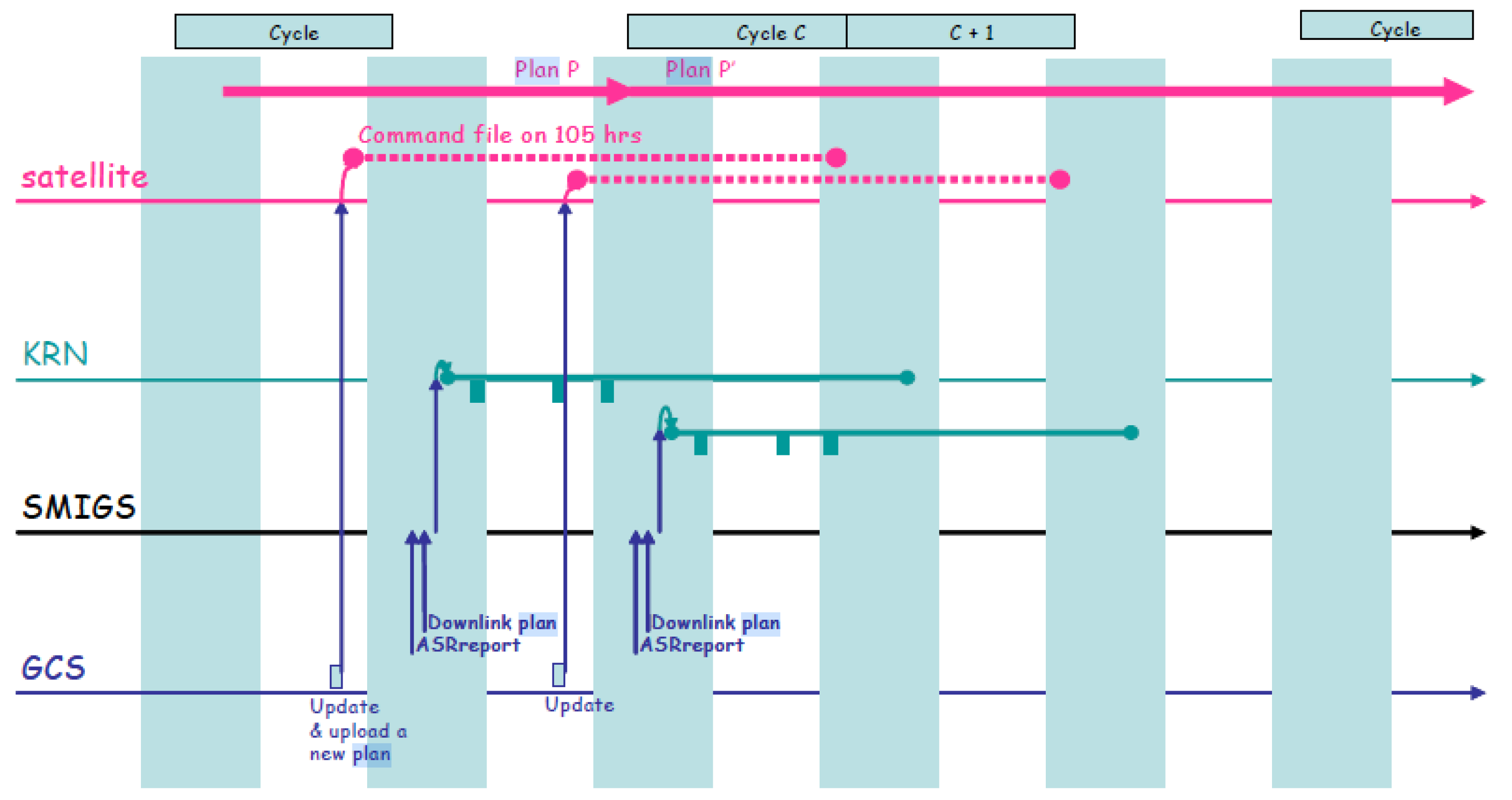
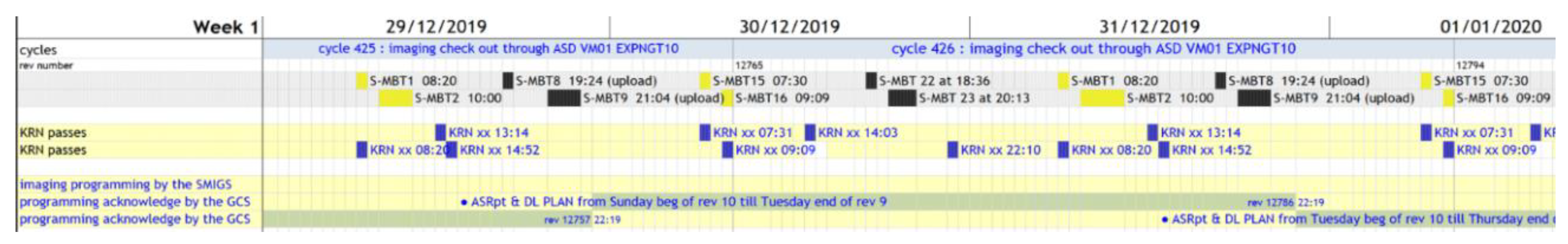
3.2.2. Scientific Mission Programming

The nominal scientific programming is under GCS responsibility, who provides a Downlink Plan file (DLPlan) and supplies, among other information, orbits for X-Band Ground Receiving Stations, transmission times, acquisition sites and auxiliary data.

The passes pace the update of the scientific command file over the S band earth terminal, thrice a week for VM01, on Tuesday, Thursday and Sunday. GCS performs an orbit determination based on the most recent GPS fixes provided either in S band or X band telemetry. At every active S band pass, GCS uploads to the satellite an updated command file, and provides SMIGS with an acquisition set report (ASR). Upon reception, SMIGS checks the downlink plan is compliant with the relevant ASD. In addition to providing the DLPlan, the GCS computes nominally the orbit, and sends nominally once a day to Kiruna an email with the orbital elements, in the form of a Two Line Elements (TLE) file. Each TLE is time stamped at KRN AOS (acquisition of signal) minus 10 min. KRN ground station uses those TLEs to compute the antenna pointing elements. Examples are given in the Figure 36 and Figure 37.

4. Data Production and Monitoring

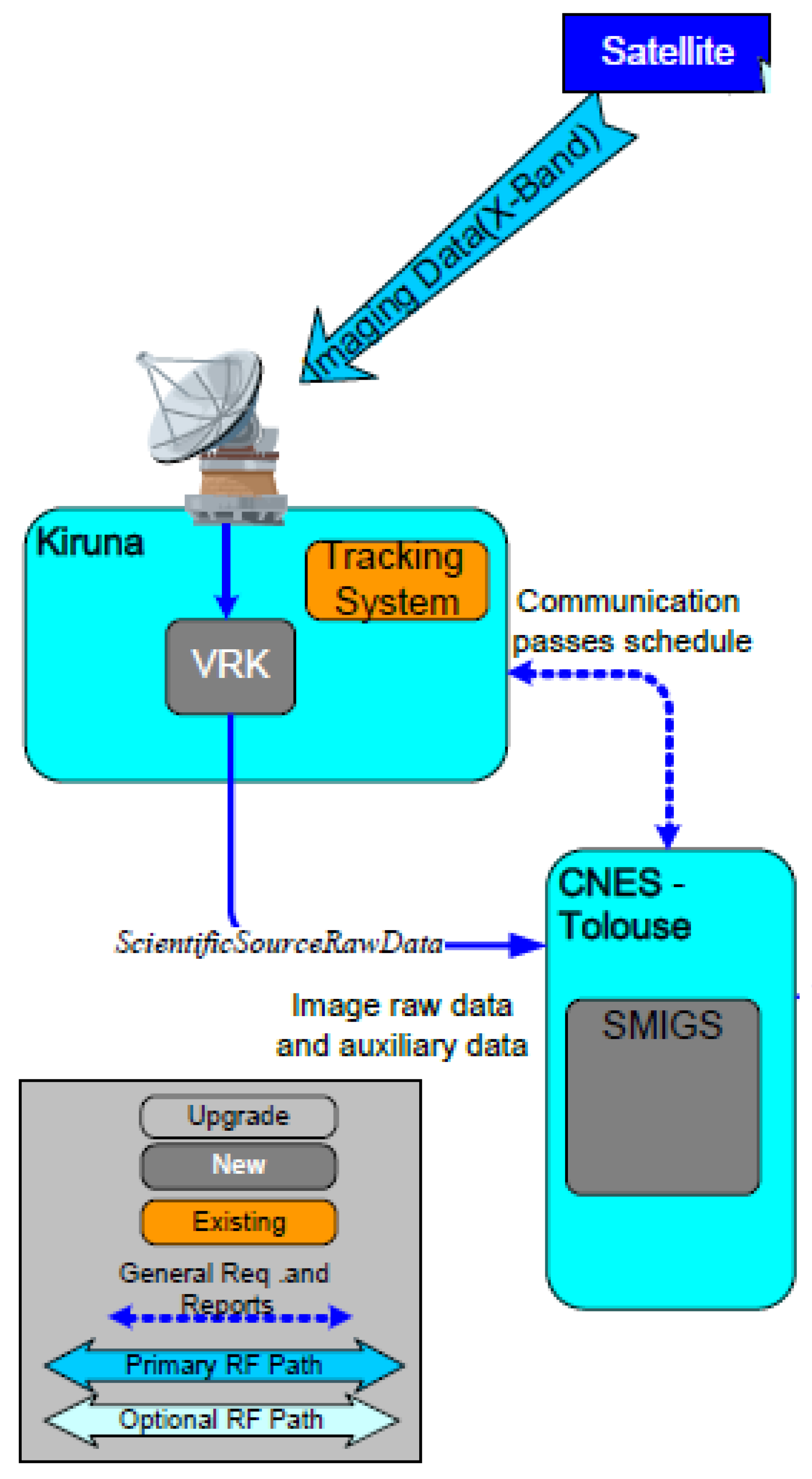
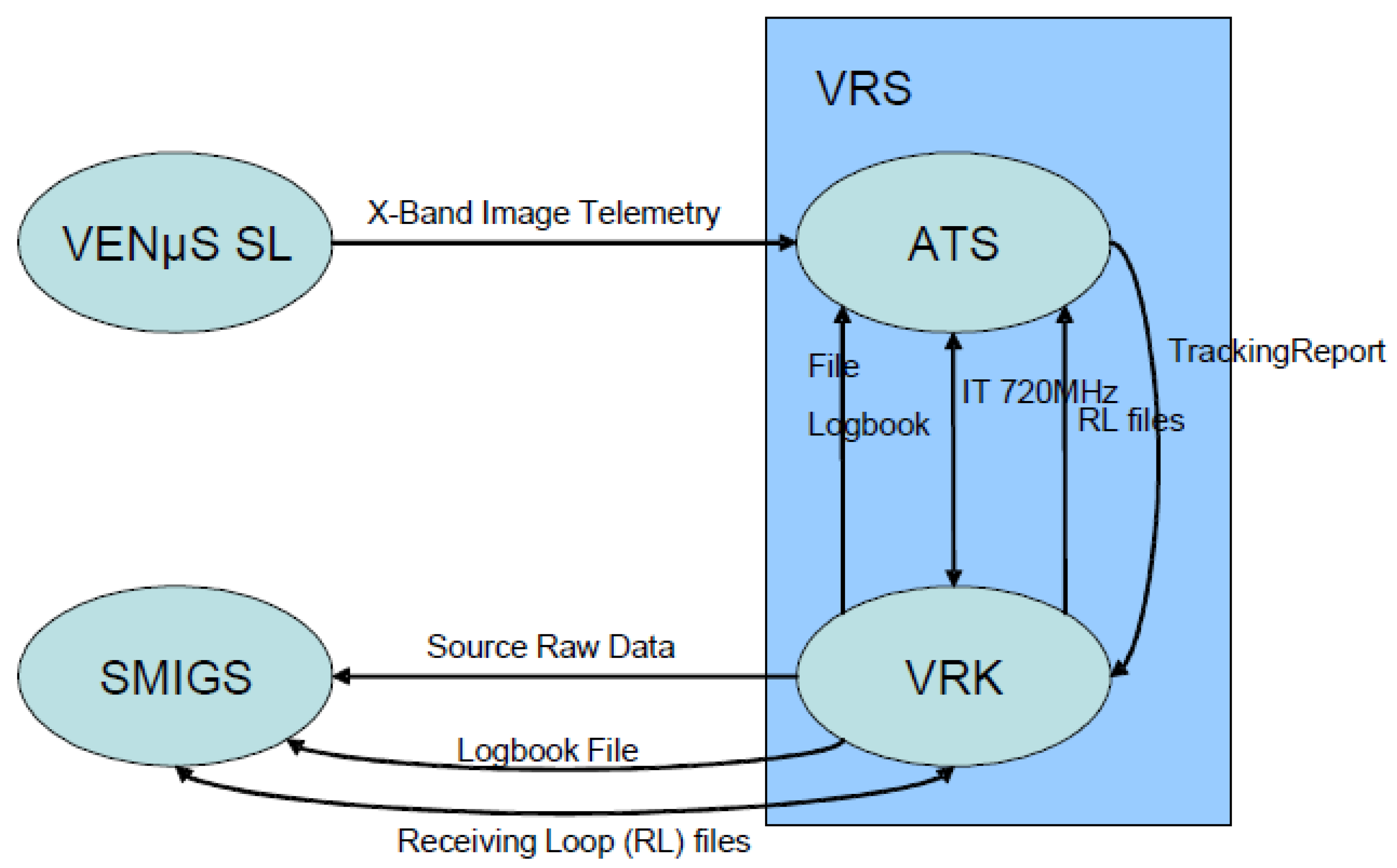
4.1. Telemetry Reception Process

The VENμS data reception is under Sweden responsibility. The Swedish Space Center Satellite Station (SSC) includes Telemetry Tracking & Command systems in S-Band, and six multi-frequency receive antenna systems in S/X-Band. VENμS passes are programmed on two of them.

The Kiruna VENμS Receiving Station (VRS) is interfacing with the SMIGS VIP that processes the data. An overview of the data reception chain is given in Figure 38. VRS unit is made of:

• the Antenna and Tracking Sub-system (ATS), for tracking the satellite, receiving telemetry signal, and supplying it in 720 MHz to the VENμS Receiving Kit (VRK);
• the VENμS Receiving Kit (VRK) (see Figure 39), for converting the signal in 140 MHz, demodulating and decoding the signal, processing Image Telemetry signal and supplying the Source Raw Data to SMIGS VIP.

Figure 38. Data reception chain overview.

Figure 38. Data reception chain overview.

The VRK is designed to carry out nominal operations automatically; nevertheless, in case of failure, operators can manually schedule a pass by connecting to the Schedule Monitor Interface.

The VRK interacts with SMIGS VIP unit by connecting the FTP server to obtain and put some files.

• From SMIGS-VIP to VRK:

  ○

  the Down Link Plan: the VRK locally archives programming file, schedules the corresponding downlinks and forwards the file to the ATS.

• In addition, from VRK to SMIGS-VIP:

  ○

  the Down Link Report: the report file produced by the VRK after each downlink to provide its detailed status;

  ○

  the Tracking Report: the report file is created by the ATS when tracking the spacecraft;

  ○

  the Scientific Raw Data: data are sent to the VIP server by X Band.

Once Scientific Raw Data are received in the VIP unit, the inventory chain is automatically launched to build raw images and catalog the inventory products.

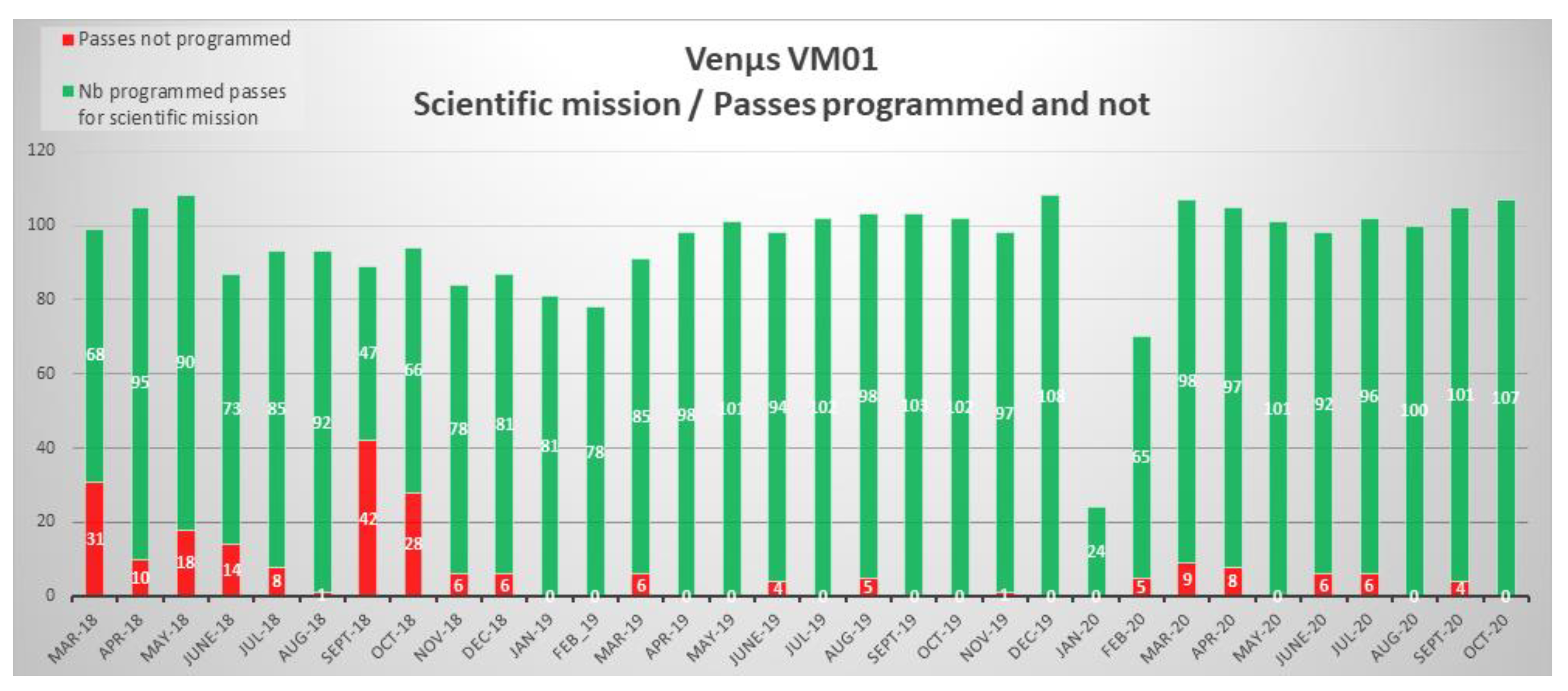
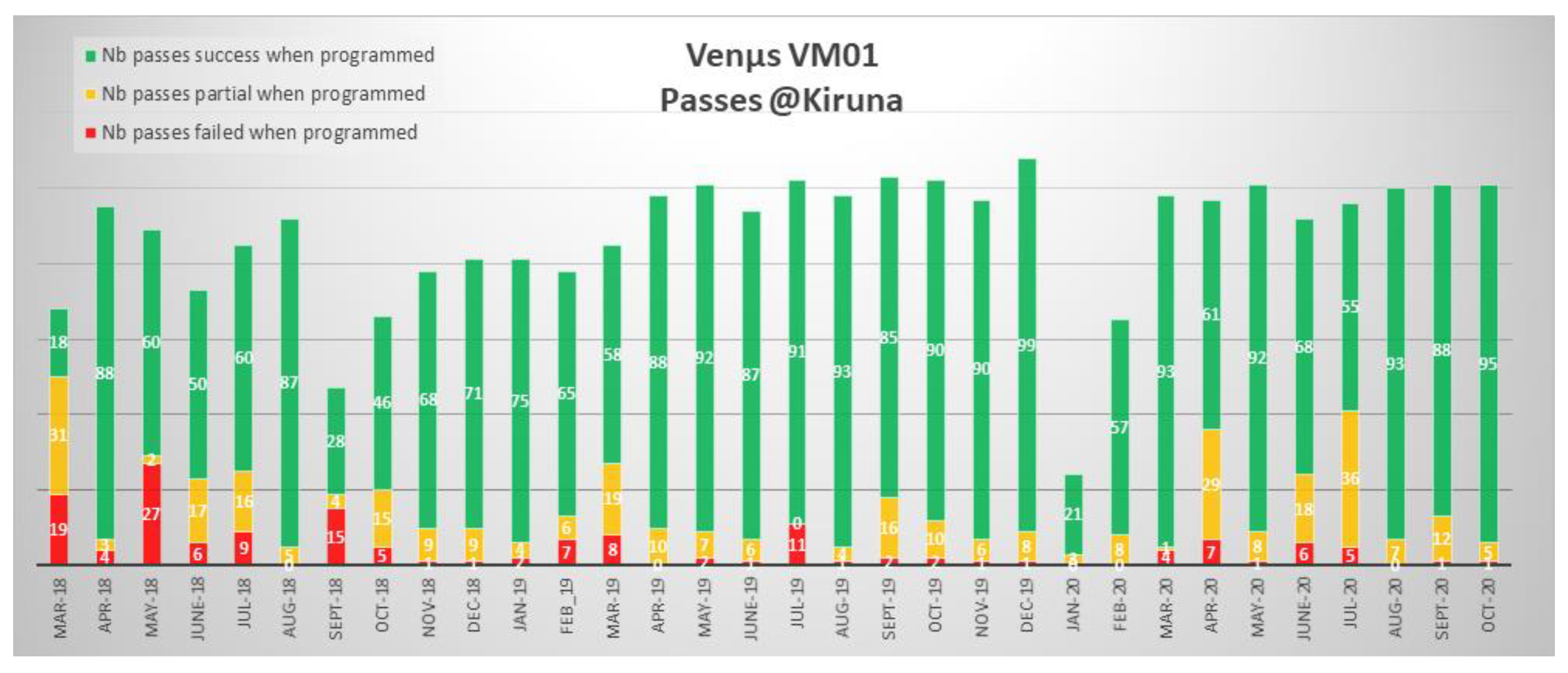
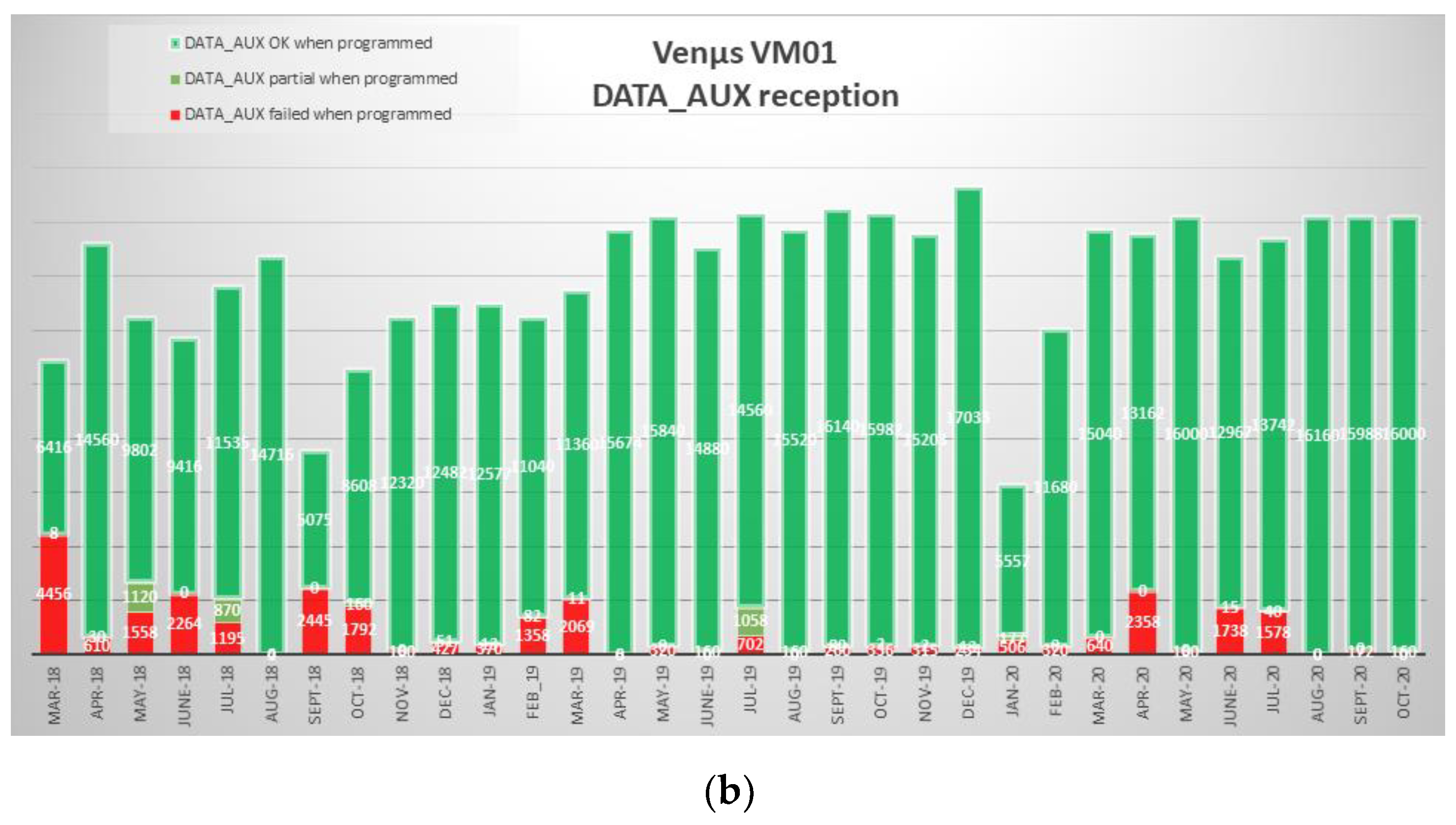
4.2. Telemetry Reception Statistics

The following figures illustrate the statistics in terms of station programming or in terms of telemetry downloading quality. Overall, VIP was able to retrieve (green part of the graph):

• an average of 86% of theoretical data (programmed and not programmed) for all VM01 duration;
• 92% of theoretical data if we only consider the last year of operations;
• 94% of programmed data for all VM01 duration.

The next figure (Figure 40) shows statistics on the evolution of the image telemetry receiving and processing since the beginning of the VM01 routine mission (March 2018–October 2020).

For various reasons, it may happen that the data reception at Kiruna station is not fully completed, and only some telemetries are received: sometimes, auxiliary data are missing or are not complete, and sometimes the image telemetries are not compliant. In these cases, the status of the station pass programmed is “Partial” or “Failed”. The Figure 41 and Figure 42 present the statistics for VM01 per month.

4.3. Operationnal Processing Chains

Two units of the SMIGS Center are in charge of processing VENμS products:

• VIP for Level-1 products;
• THEIA for Level-2 and-3 products (except for Israeli sites which are under Ben Gurion University responsibility).

4.3.1. VENμS Image Processor (VIP)

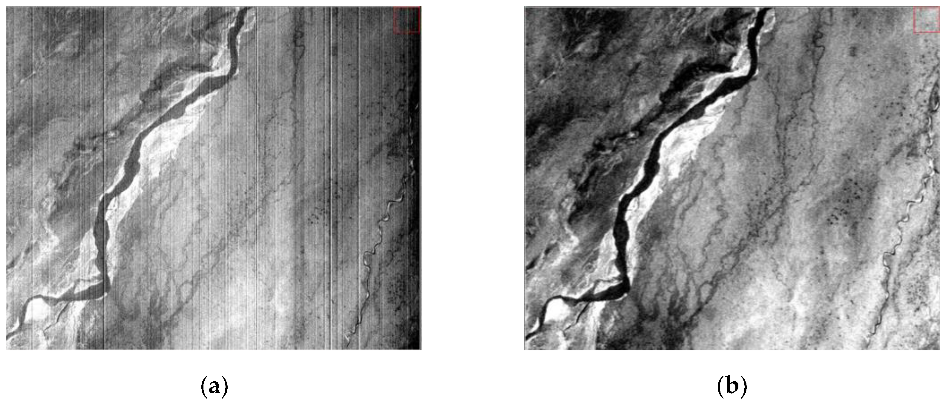
In addition to scientific mission programming, the VIP Unit is in charge of Level-0 and Level-1 processing, with characteristics described in the

Table 1. Characteristics of VENμS products levels.

Level	Radiometry	Geometry	User
0	Raw	Raw	Internal
1A	Radiometric corrections	Raw	Internal
1	Radiometric corrections	Multi spectral registration Cartographic projection	Provided to scientists

.

A Level-0 product is made of the image data without any processing, only with a system localization.

A Level-1A product is processed with the same geometric that Level-0. Only some radiometric corrections are conducted:

• equalization;
• interpolation of outlying detectors;
• persistance correction;
• restauration.

The Level-1 processing chain generates products automatically on telemetries reception.

4.3.2. THEIA

THEIA is a data and services center specializing in land surfaces. Theia offers a portfolio of products and associated services for the scientific community and public bodies through its web portal [29]. This data infrastructure pulls together a number of organizations, including CNES.

For VENμS, THEIA is in charge of Level-2 and Level-3 processing, and Level-1 to Level-3 distribution (see Figure 43).

The Level-2 processing chain takes Level-1 valid products coming from VIP (VENμS Image Processing center), using MAJA-3 software. Beyond 80% cloud cover, the Level-2 is considered as not valid and is cancelled. All sites are processed with the same configuration parameters, except sites located at high latitudes, which have a specific configuration for snow detection. A complete reprocessing is planned with MAJA-4, taking into account meteorological data.

The Level-3 processing chain generates two syntheses per month, on day 1 and 16, using WASP software. The configuration for VENμS is a 23-day window around the chosen date, corresponding to two 11-day half-windows. At least two Level-2 valid products must be available inside the window for the Level-3 product to be processed.

For the whole VENμS mission, 78,040 products are available, including 30,631 Level-2, and 1330 Level-3. The processing of Level-3 product is currently in progress.

4.4. Image Quality Monitoring

VENμS products’ image quality is monitored through an expertise center, in CNES premises, named VIQ (VENμS Image Quality). The following paragraphs describe the VIQ itself, and the radiometric and geometric processes which allow us to maintain an optimal image quality for the Level-1 products delivered to THEIA land data center. Additionally, some statistics on the different levels of products (from Level-1 to Level-3) are introduced, to provide an idea of the VENμS data series completeness and quality.

4.4.1. VENμS Image Quality Expertise Center (VIQ)

VIQ Missions

In the frame of the VENμS SMIGS, the image quality of VENμS products is maintained through the VIQ (VENμS Image Quality expertise center).

The missions of the VIQ are to assess and to accurately and regularly monitor the imaging system performances (through the performances budget), to generate and to deliver to the VIP all the data needed to deliver products consistent with the scientific requirements, and to provide facilities to analyze anomalies and to elaborate corrections and workarounds.

One of the key notions of this image quality monitoring is the ground image processing parameters tuning. Ground image processing parameters (GIPP) are key parameters to process raw telemetry up to Level-0, Level-1 and Level-2 products. These GIPP are set and tuned on VIQ side, and delivered to the Level-0, Level-1 and Level-2 processing chains, either on VIP side or on THEIA side. Concerning the VENμS mission, these GIPP can be applied taking into account both a temporal and a spatial dimension. These spatial and temporal applicability options, together combined, are the basis of VIP processing accuracy. The Level-1 processing chain is thus able to take into account geographic and temporal specificities, which allow us to have a system delivering products with a high level of image quality, wherever and whenever they are acquired.

It can be noted that, additionally to these ground parameters, which are highly modifiable, some on-board tuning is also possible and monitored on the VIQ side. The ATPSET (Acquisition Technical Parameters SET) defines, for each spectral band of the instrument, the on-board characteristics of the detectors (offset, video gain and number of TDI stages) in order to obtain the best dynamic range of the instrument. The main goal is to avoid saturations and negative values in final products. As these parameters are directly applied on-board, the notion of applicability period does not have the same meaning as for the ground parameters used in the processing chain (the parameters are applied since they are uploaded on board). However, a spatial dependence of these ATPSET can be defined, which allows us to apply different sets of parameters according to the geolocation of the acquisitions.

VIQ Breakdown

As shown in Figure 31, the VIQ is an expertise center, part of the VENμS French image ground segment. The VIQ is a system (software and hardware) providing a database and a pool of tools to compute, monitor and maintain the radiometric and geometric performances of VENμS products.

Combined with the VIP and other expertise systems (such as MUSCLE (Multi Sensor CaLibration Environment) dedicated to the radiometric calibration of different instruments), the VIQ drives an image quality loop, designed to monitor and maintain VENμS performances. The goal is to deliver to final users Level-1 products consistent with the scientific requirements [30].

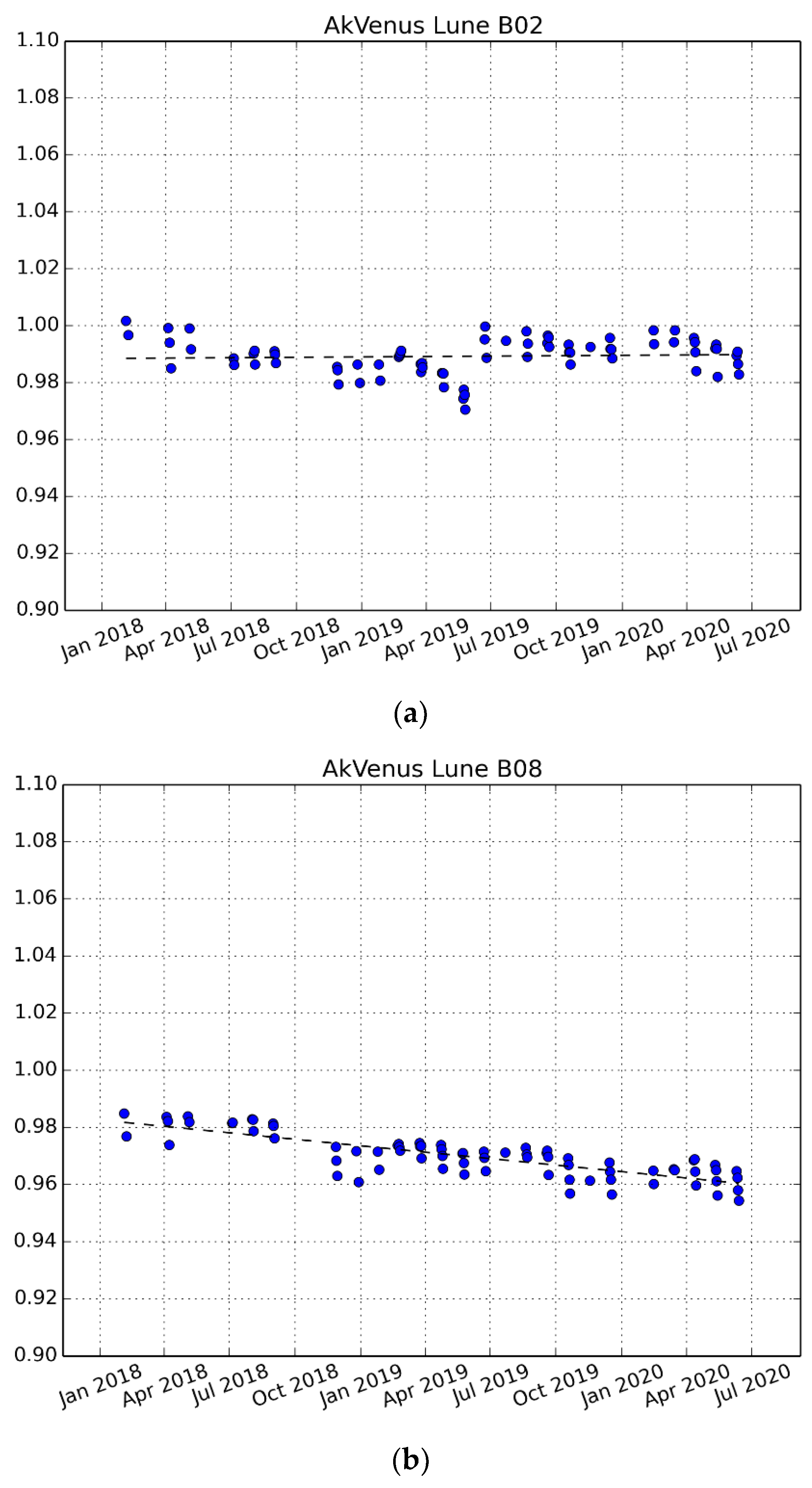
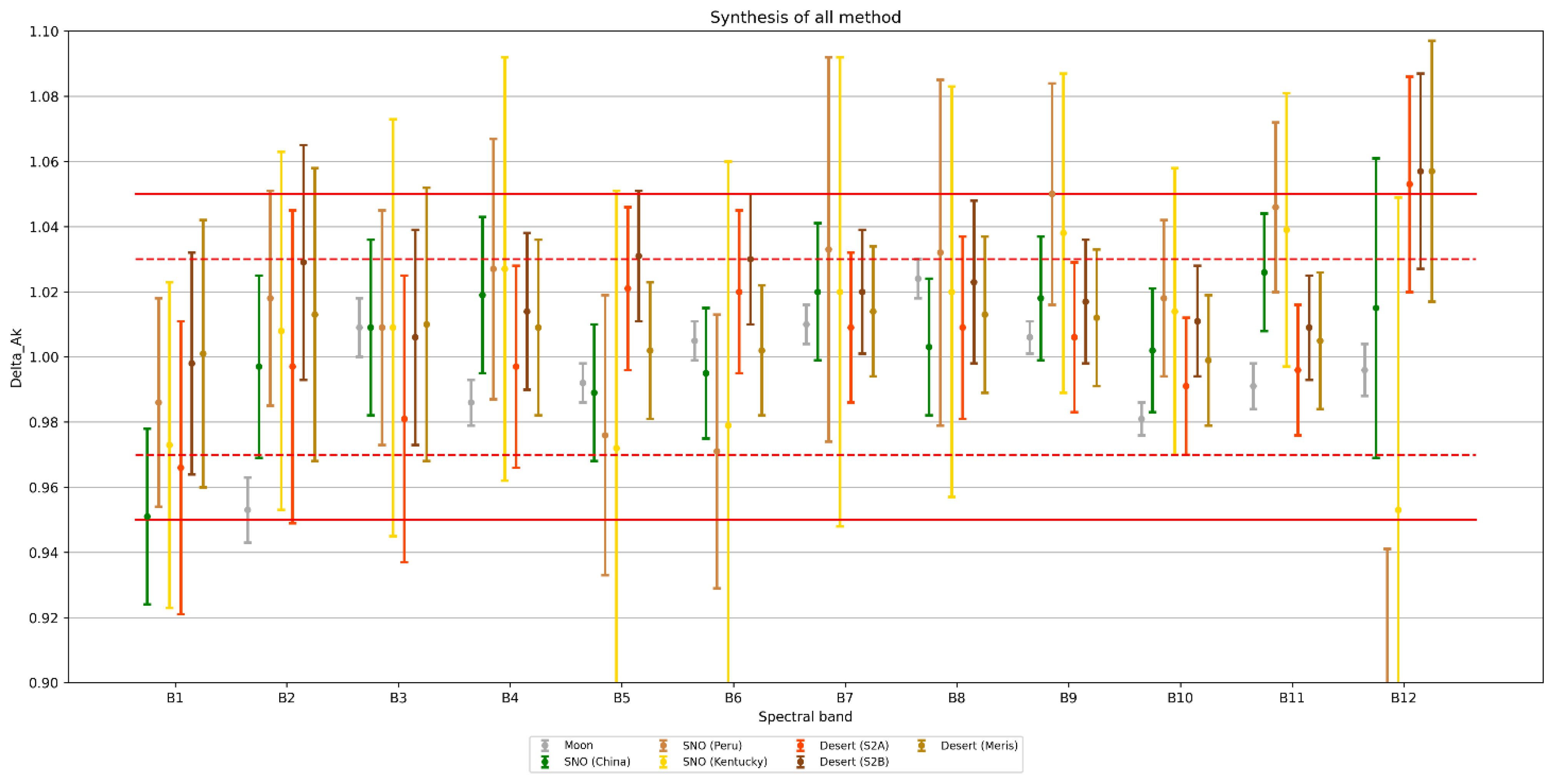
4.4.2. Radiometry Monitoring Activities

If we consider image quality monitoring, the first thematic to be considered is the radiometric performances monitoring. The following paragraphs detail the main radiometric performances monitoring activities carried on thanks to the VIQ expertise center.

Simultaneous Nadir Observation: Sentinel2 Inter-Calibration Expertise

Every month, knowing the SENTINEL2 and VENμS orbits, the conjunction opportunities are computed in order to check the dates where a couple of acquisitions (VENμS, SENTINEL2A or B) exists. For all these dates, SENTINEL2 L1C and VENμS L1 are downloaded and ingested in VIQ database. After that, specific operations are processed to cross-calibrate VENμS and Sentinel2 data. The two following figures (see Figure 44) illustrate a typical couple of acquisitions Sentinel-2A and VENμS, on the SNOCHINA VENμS site.

Desert Calibrations

Another radiometric monitoring activity concerns the processing of calibrations sites acquired over desert areas.

Every month, all the acquisitions over four different desert sites during the previous month are processed by the VIP up to Level-1 and delivered to the VIQ. Then, an accurate analysis is made on the VIQ side to keep only the acquisitions with no cloud coverage. As shown in the Figure 45, this choice can be tricky because some cloud coverage is very thin and difficult to estimate. In the examples of this figure, only the acquisitions of 2 and 4 June 2020 were finally selected for the radiometric calibration processing.

At this point, the chosen selection of Level-1 is processed through dedicated tools in the VIQ. Average measurements, for each spectral band, are thus produced and delivered to the MUSCLE cross calibration facility.

Equalization and Instrument Noise Monitoring

In terms of radiometric monitoring, radiometric noise is a key parameter. The assessment of equalization and instrument noise performances is based on the processing of desert calibration and two different geographic sites over Arctic and Antarctic areas.

For these specific snow sites, it is important to select, for the processing, a homogeneous area to exclude clouds and landscapes specificities. The following figure (see Figure 46) shows an example of acquisition over EGAANTAR site. Only the homogeneous part of the Level-1A product (in green) is selected operationally for processing (extract and zoom parts of this area can be seen in the right of the image, to have an idea of what means “uniformity” at the spatial resolution of VENμS).

4.4.3. Geometry Monitoring Activities

Geographical Sites Characteristics Management

Even if the sites (coordinates, satellite attitude for acquisitions, etc.) are mainly managed on the VIP side, some characteristics are dealt with on the VIQ side. This is the case for the projections grids which are computed on VIQ side. The VIQ also produces the digital terrain models (DTM) specific to every site. These DTM are processed from SRTM for almost all sites.

One exception concerns extreme latitudes (for example CHERSKII and SVALBAR1), for which Planet Observer is used [31]. Another exception is for the Himalaya site KHUMBU, processed with a dedicated DEM (High Mountain Asia DTM from NASA [32]). Indeed, orthorectification issues in KHUMBU L1 images were highlighted by users, due to a change in VENμS satellite attitude between two acquisitions. These attitude changes and a poor quality of SRTM DTM over Everest area lead to significant errors in multi-temporal registration. Therefore, it was decided to change the DTM on KHUMBU site by using the High Mountain Asia (HMA) digital elevation model, produced and distributed by the NASA National Snow and Ice Data Center Distributed Active Archive Center (NSIDC DAAC).

The Figure 47 shows an illustration of a Level-1 DTM for JORDANA site. These data are delivered to the VIP to be taken into account in Level-1 processing chain, as part as reference data (in association with the reference image).

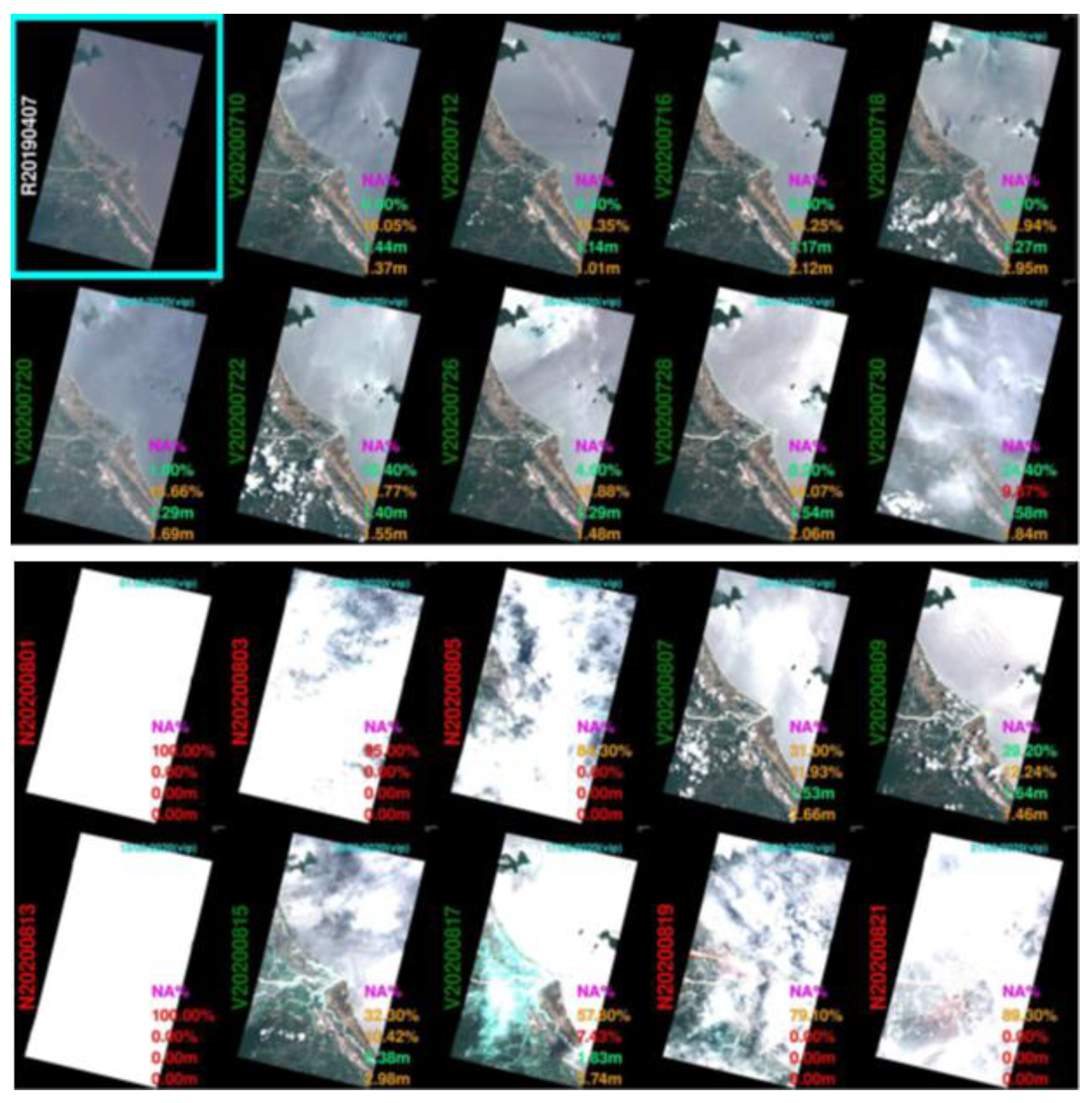
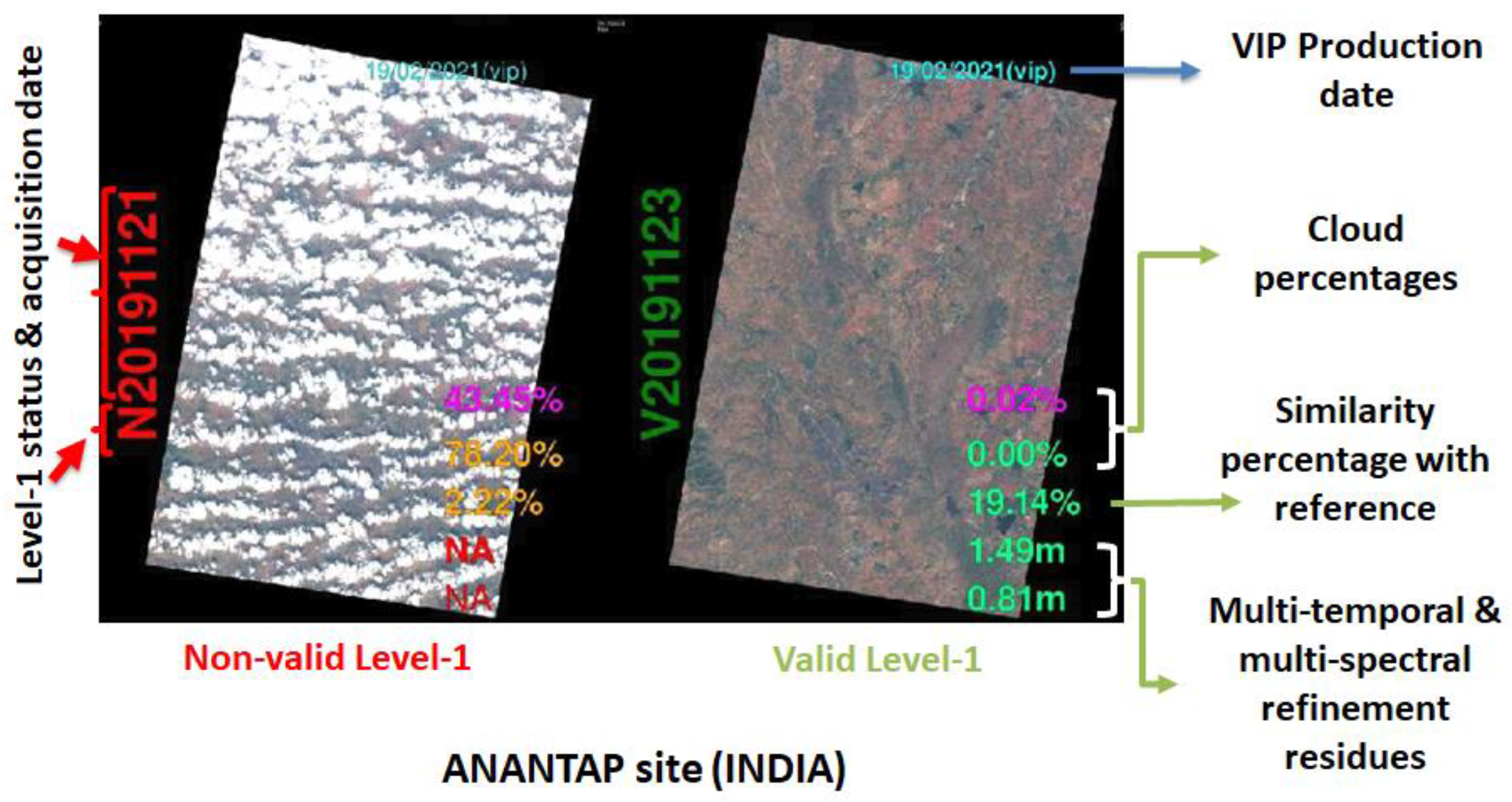
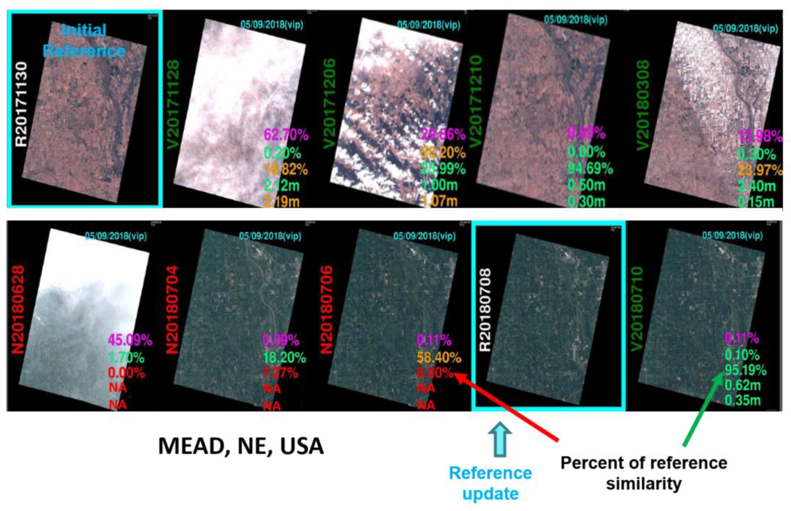
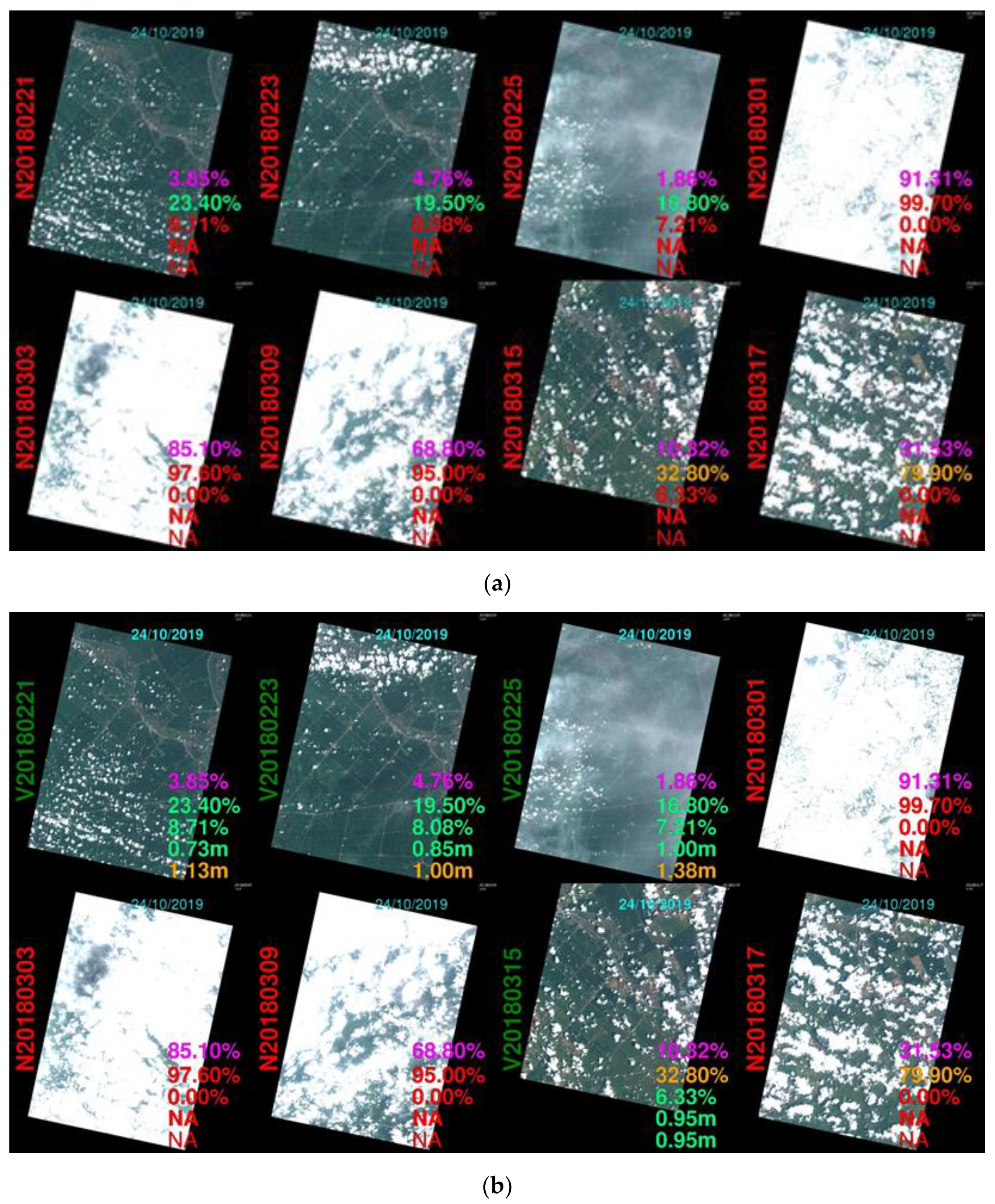
Reference Image Management

• Reference Image Definition

As a reminder, reference image is a key data for VENμS image processing. It is the basis of Level-1 data time series, i.e., Level-1 products perfectly registered one to the others. For each site, a reference image is a specific mono-spectral image upon which every acquisition is registered on. This image is applicable over a period of time depending on the site landscape.

For a specific acquisition (date and site), the VIP delivers to the users (through THEIA land data portal) a Level-1 product only if it is declared “valid”, which means that its multitemporal and multispectral registration performances comply with the scientific requirements and that this product is correctly included in a time series of spatially registered Level-1 products. As this spatial registration is the result of the correlation success with the reference image, the validity of reference data is accurately monitored in order to maintain the image quality of the Level-1 products and the number of valid products delivered to the users. Consequently, this reference image is very important for multi-temporal and multi-spectral registration performances.

• Reference Image Monitoring

On the VIQ side, a specific activity is to monitor the reference image and the evolution of the correlation between this reference and each current acquisition. The reference image being specific to each site, this time series monitoring must be conducted for each scientific site.

For this monitoring, thumbnail mosaics are used to obtain an immediate global vision of the data time series for the studied site. The figure below (Figure 48) is an example for the HOIAN site.

The Figure 49 shows the detailed information provided on each acquisition. Various statistics allow us to qualify the validity and the image quality of the product. The percentage of valid correlation points between reference and acquisition, which defines the quality of the temporal registration, is very important to monitor the quality of the reference image and to identify if it needs to be updated.

Using the results provided by this monitoring, the importance of the seasonal updating of the reference image for some specific sites is highlighted.

• Seasonal Updating

The seasonal updating of the reference image is a key activity in image quality monitoring to maintain both a high number of valid Level-1 delivered to the users and multi-temporal and multi-spectral registrations performances within the scientific requirements.

The Figure 50 is a practical illustration, for the MEAD site (Mead, NE, USA), of the importance of this monitoring, and demonstrates the dependence of the reference image correlation results with the landscape and its seasonal evolution.

On the top of the figure is presented the wintertime series of Level-1 products, all declared valid thanks to good correlation statistics with the first reference image (enhanced in a blue square), which is a winter acquisition. The three left-bottom quicklooks correspond to summer acquisitions, also processed with the same winter reference image. The landscape is, visually, extremely different in comparison with the top-left reference winter acquisition. In these cases, the similarity percentage with this reference is very low (between 0 and 8%). The consequence is that these products are declared not valid, despite the fact that wo of the three images do not have any cloud.

A new reference image (summer acquisition of 8 July 2018) is thus built and introduced in the processing chain. After this reference update, all the acquisition which are acquired are registered on this summer reference image. The registration with the reference is consequently very good and the product is declared valid. Therefore, these numerical results demonstrate the importance of the reference image monitoring. For each site, with the knowledge of the landscape evolution through the year, various seasonal reference image should be built and applied at the seasonal transition dates, in order to deliver the maximum number of valid Level-1 products to the users.

Geometric GIPP Tuning

As shown in the previous paragraph, the seasonal updating of the reference image is crucial in order to deliver to the users the maximum number of valid Level-1 products.

Nevertheless, in some cases (for example, for uniform landscapes which do not evolve temporally), this tuning is not possible. Another important parameter can thus be tuned: the correlation percentage threshold, being part of the decision to declare valid or not the Level-1 product. If the similarity percentage of valid correlation points between an acquisition and its reference image is below a specific threshold, the Level-1 product is not valid.

Typically, this threshold is set to 10% in the nominal GIPP. For some difficult geographical sites with very homogeneous landscape (forest sites or snowy sites), this threshold specific lower percentages can be applied to increase the number of valid Level-1 products.

The two next figures (see Figure 51) illustrate this situation for ANGIANG site. The first figure shows that no Level-1 is declared valid with the 10% threshold. The second figure is the same time series after a reprocessing, with the application of a specific GIPP with a 6% threshold. The less cloudy products become valid and can thus be delivered to users.

4.5. Production Statistics (L0, L1, L2, L3)

4.5.1. Raw (Level-0) Inventory Products

The Figure 52, presented below, represents the number of raw inventory products and their location.

Of course, most of the sites have the same average number of telemetries available for Level-1 processing (above 400 products). Nevertheless, for some sites, fewer inventory products are available, for various reasons. On one hand, a possible reason is that some sites have been added more recently (for example, LERIDA1 and LERIDA2 in Europe) and consequently have a shorter time series. On the other hand, some sites have been acquired at the beginning of VM01, but, for scientific purposes, have been abandoned (evolution of the needs, on board memory space need for new acquisitions asked by scientists, etc.) or have changed in terms of geographic coverage (but a slight change triggers, by design, the definition of a new site, etc.). Various situations exist: DDUANT has rapidly changed to DUANTNEW, whereas REDRIVER was acquired for 8 months (from April to November 2019) before being modified to another footprint REDRIVR2 (observed afterwards for 11 months to October 2020).

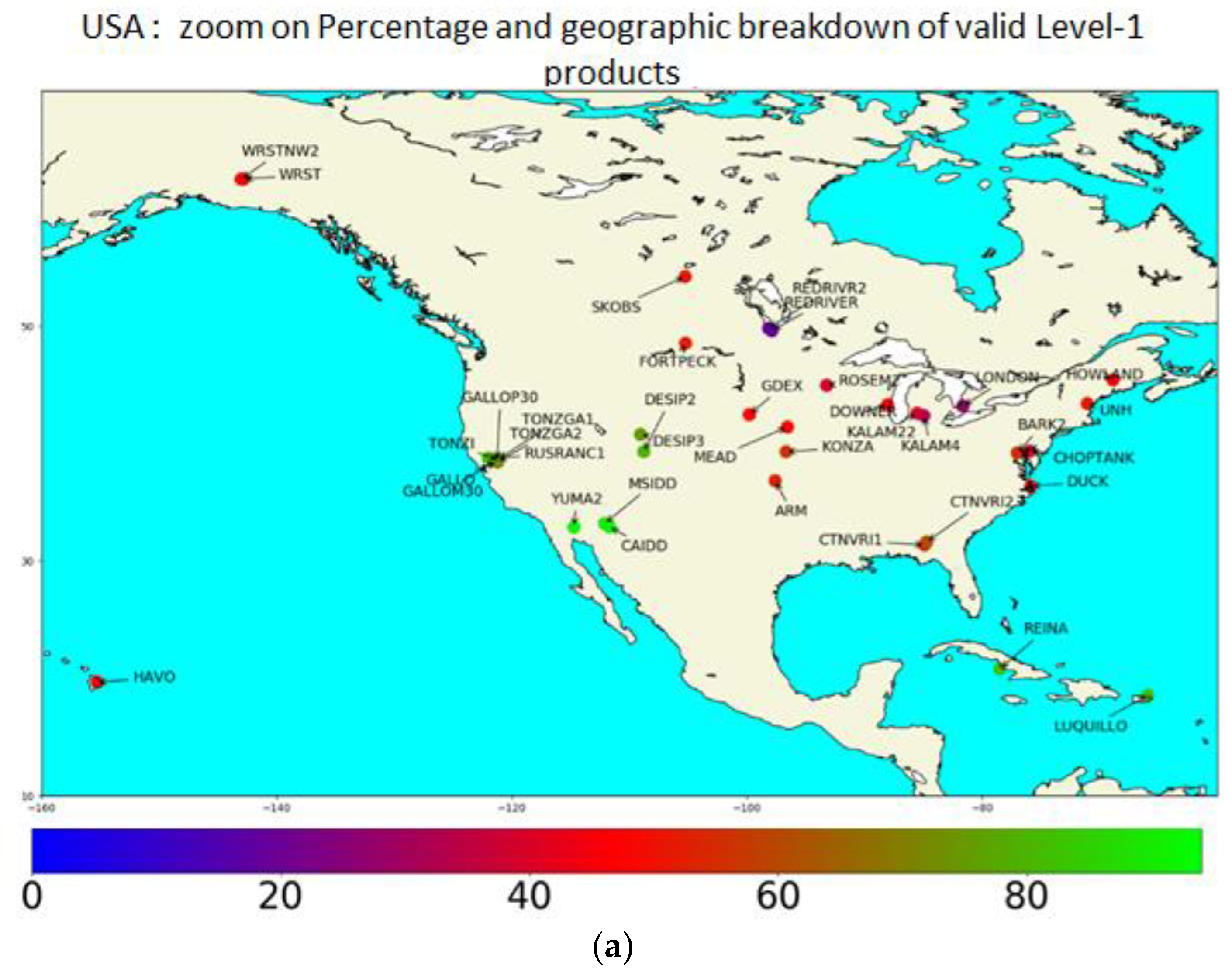
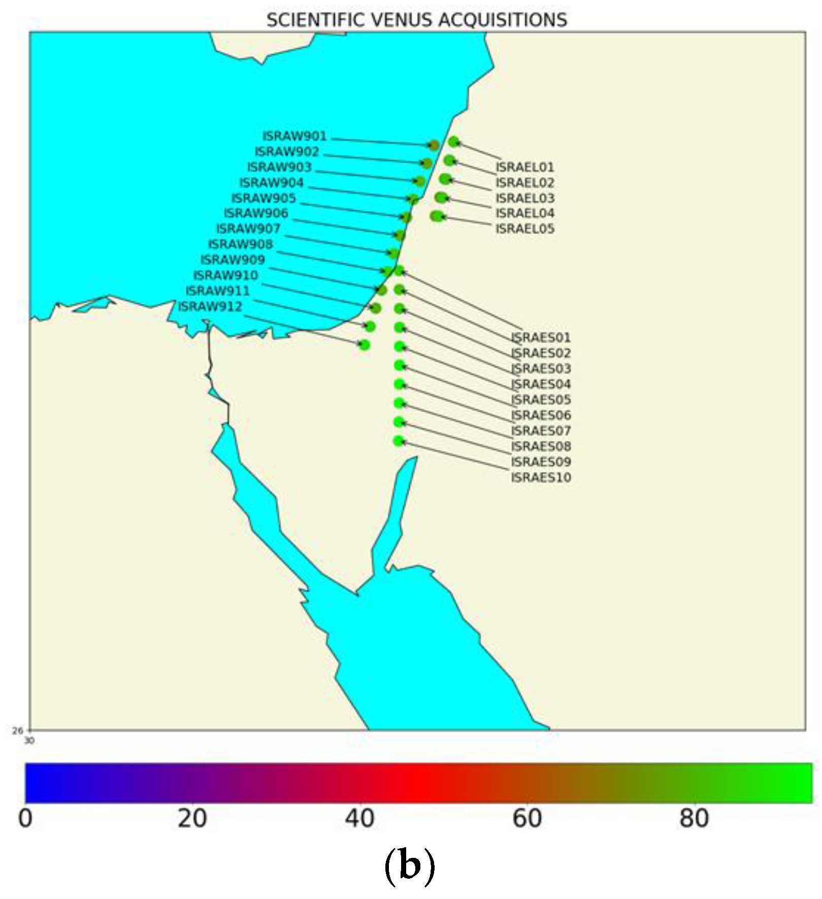
4.5.2. Level-1 Processing statistics

Level-1 products are processed from inventory data, and are qualified as valid or invalid, taking into account the global cloud coverage and geometric image quality statistics.

Considering the global Level-1 processing, 99.6% of inventory products were processed up to Level-1 (valid and non-valid). Among them, 56.53% of valid Level-1 products were delivered to users (either on THEIA land data portal or by Ben Gurion University for Israeli sites).

The figures below (see Figure 53) illustrate the geographic breakdown of the number and percentage of Level-1 valid products available, at the end of VM01 mission.

These maps show a heterogeneity between the percentages of valid Level-1 products available. This is linked to the climatic environment of the site and the global cloud coverage of the site, highly dependent on the geolocation and the climatology of the site. The Figure 54 illustrates this situation considering two different countries: USA and Israel. On one side, between northeast and southwest USA, we can clearly see the increase of the percentage of available Level-1 products. On the other side, for Israel, given the size of the country and its geographic position, the percentage of valid Level-1 products is both high and stable for all the tiles available for the different sites.

4.5.3. Level-2 Processing statistics

Level-2 products are generated from the Level-1 valid products acquired immediately before and after. Considering the global Level-2 processing by THEIA (excluding Israeli sites which are not available on THEIA land data portal), 81.75% of Level-2 were processed and delivered to users from the Level-1 valid products (Level-2 are not processed from non-valid Level-1 products).

The following Figure 55 illustrates the geographic breakdown of the number and percentage of Level-2 products avlable, at the end of VM01 mission.

As for Level-1, a climatic/geographic dependency is clearly visible in the percentages of available Level-2 products.

4.5.4. Level-3 Processing Statistics

At the time of writing this article, the final VM01 reprocessing was still ongoing, including the global Level-3 reprocessing. As no VENμS site has been entirely reprocessed at Level-3, no relevant statistic could be provided in this article.

5. Conclusions

The main objective of the VENμS mission is to provide a time series with a high revisit period, a high ground resolution and stable acquisition angles. This combination of these revisit periods and ground resolution is innovative with respect to other similar earth observation satellite such as Sentinel-2 or Landsat 8. The increasing of the revisit period is crucial to limit the impact of cloud-coverage on the applications, such as detailed land-cover mapping, agri-environment policies, water management, vegetation primary productivity and yield estimates and to capture rapid phenomena. In this context, VENμS products offer an undeniable added value to explore the benefit of expanding the time rate of high-resolution acquisition in visible and near infrared spectral bands.

This paper provides a description of the VENμS instrument and products, the status of the calibration and performance assessment of each product level at the end of the VM01 phase, the overview of the system, operation and image quality monitoring activities and the final statistics of the production of data acquired during the first phase of the VENμS mission.

The presented results are very satisfactory and show the good performance of the VENμS products in terms of both radiometry and geometry for each product levels. Thanks to numerous radiometric and geometric vicarious calibration methods, the performances are monitored accurately over time all along the VM01 phase. A regular update of the image processing parameters allows us to retain an excellent image quality.

Finally, this first VM01 phase generated an important archive of thousands Level-1 products over more than 150 scientific sites. The 2-day revisit deeply increases the capacity to process Level-2 and Level-3 products. In order to go further in this breakthrough of combining high revisit and high ground resolution, VENμS has just begun a new mission phase, VM05. In only a few months, VENμS satellite reached another orbit at 560 km of altitude. This new orbit provides the opportunity to have a daily revisit and a ground resolution of about 4 m over a hundred scientific sites. These new characteristics reinforce VENμS as a demonstrator for future missions of earth observation.

References

1. Kimes, D.S. Dynamics of directional reflectance factor distributions for vegetation canopies. Appl. Opt. 1983, 22, 1364–1372. [Google Scholar] [CrossRef]
2. Townshend, J.R.G. Global data sets for land applications from the Advanced Very High Resolution Radiometer: An introduction. Int. J. Remote Sens. 1994, 15, 3319–3332. [Google Scholar] [CrossRef]
3. Maisongrande, P.; Duchemin, B.; Dedieu, G. VEGETATION/SPOT: An operational mission for the Earth monitoring: Presentation of new standard products. Int. J. Remote Sens. 2004, 25, 9–14. [Google Scholar] [CrossRef]
4. Justice, C.O.; Vermote, E.; Townshend, J.R.G.; Defries, R.; Roy, D.P.; Hall, D.K.; Salomonson, V.V.; Privette, J.L.; Riggs, G.; Strahler, A.; et al. The Moderate Resolution Imaging Spectroradiometer (MODIS): Land remote sensing for global change research. IEEE Trans. Geosci. Remote Sens. 1998, 36, 1228–1249. [Google Scholar] [CrossRef] [Green Version]
5. Dedieu, G.; Cabot, F.; Chehbouni, A.; Duchemin, B.; Maisongrande, P.; Boulet, G.; Pellenq, J. RHEA: A micro-satellite mission for the study and modeling of land surfaces through assimilation techniques. In Proceedings of the EGS-AGU-EUG Joint Assembly, Nice, France, 6–11 April 2003; p. 8138. [Google Scholar]
6. Dedieu, G.; Hagolle, O.; Karnieli, A.; Ferrier, P.; Crébassol, P.; Gamet, P.; Desjardins, C.; Yakov, M.; Cohen, M.; Hayun, E. VENµS: Performances and first results after 11th months in orbit. In Proceedings of the IGARSS 2018—2018 IEEE International Geoscience and Remote Sensing Symposium, Valencia, Spain, 22–27 July 2018; pp. 7756–7759. [Google Scholar] [CrossRef]
7. CEOS: Committee on Earth Observation Satellites. Analysis Ready Data for Land, Product Specification, Surface Reflectance. Version 5.0, June 2020. Available online: https://ceos.org/ard/ (accessed on 21 June 2022).
8. Dick, A.; Gamet, P.; Marcq, S.; Dedieu, G.; Hagolle, O.; Crebassol, P.; Raynaud, J.-L.; Hillairet, E.; Enache, S.J. VENµS Commissioning Phase: Specificities of Radiometric Calibration. In Proceedings of the IGARSS 2018—2018 IEEE International Geoscience and Remote Sensing Symposium, Valencia, Spain, 22–27 July 2018; pp. 4320–4323. [Google Scholar] [CrossRef]
9. Dick, A.; Dedieu, G.; Hagolle, O.; Raynaud, J.-L.; Pelou, S.; Burochin, J.-P.; Erudel, T. VENμS: VM01 Final Radiometric Assessment and Future Phases. In Proceedings of the IGARSS Proceedings, Brussels, Belgium, 11–16 July 2021. [Google Scholar]
10. Lacherade, S.; Fougnie, B.; Henry, P.; Gamet, P. Cross Calibration Over Desert Sites: Description, Methodology, and Operational Implementation. IEEE Trans. Geosci. Remote Sens. 2013, 51, 1098–1113. [Google Scholar] [CrossRef]
11. Meygret, A.; Blanchet, G.; Colzy, S.; Gross-Colzy, L. Improving ROLO lunar albedo model using PLEIADES-HR satellites extra-terrestrial observations. In Proceedings of Earth Observing Systems XXII; SPIE: San Diego, CA, USA, 2017; Volume 10402, p. 104022A. [Google Scholar] [CrossRef]
12. Marcq, S.; Meygret, A.; Bouvet, M.; Fox, N.; Greenwell, C.; Scott, B.; Berthelot, B.; Besson, B.; Guilleminot, N.; Damiri, B. New Radcalnet Site at Gobabeb, Namibia: Installation of the Instrumentation and First Satellite Calibration Results. In Proceedings of the IGARSS 2018—2018 IEEE International Geoscience and Remote Sensing Symposium, Valencia, Spain, 23–27 July 2018; pp. 6444–6447. [Google Scholar] [CrossRef]
13. Frouin, R.; Sei, A.; Hauss, B.; Pratt, P. Operational in-flight calibration of NPP VIIRS in the visible using Rayleigh scattering. In Proceedings of Earth Observing Systems XIX; SPIE: San Diego, CA, USA, 2014; Volume 9218, p. 921806. [Google Scholar]
14. Hillairet, E.; Enache, S.J.; Burochin, J.-P.; Dick, A.; Marcq, S.; Hagolle, O.; Raynaud, J.-L.; Gamet, P. VENµS in orbit radiometric calibration. In Proceedings of Sensors, Systems, and Next-Generation Satellites XXII; SPIE: Berlin, Germany, 2018; Volume 10785, p. 1078513. [Google Scholar] [CrossRef]
15. Gamet, P.; Fourest, S.; Sprecher, T.; Hillairet, E. Measuring, modelling and removing optical stray light from VENµS Super Spectral Camera Images. In Proceedings of the International Conference on Space Optics—ICSO 2018, Chania, Greece, 9–12 October 2018; Volume 11180, p. 111804F. [Google Scholar] [CrossRef]
16. Binet, R.; De Lussy, F.; Languille, F.; Rolland, A.; Raynaud, J.-L.; Specht, B.; Gamet, P. VENµS geometric image quality commissioning. In Proceedings of Sensors, Systems, and Next-Generation Satellites XXII; SPIE: Berlin, Germany, 2018; Volume 10785, p. 107850J. [Google Scholar] [CrossRef]
17. Hagolle, O.; Huc, M.; Villa Pascual, D.; Dedieu, G. A Multi-Temporal and Multi-Spectral Method to Estimate Aerosol Optical Thickness over Land, for the Atmospheric Correction of FormoSat-2, LandSat, VENμS and Sentinel-2 Images. Remote Sens. 2015, 7, 2668–2691. [Google Scholar] [CrossRef] [Green Version]
18. Richter, R.; Schläpfer, D.; Müller, A. An automatic atmospheric correction algorithm for visible/NIR imagery. Int. J. Remote Sens. 2006, 27, 2077–2085. [Google Scholar] [CrossRef]
19. Hagolle, O.; Huc, M.; Desjardins, C.; Auer, S.; Richter, R. MAJA Algorithm Theoretical Basis Document (Version 1.0). Zenodo 2017. [Google Scholar] [CrossRef]
20. Rahman, H.; Dedieu, G. SMAC: A simplified method for the atmospheric correction of satellite measurements in the solar spectrum. Int. J. Remote Sens. 1994, 15, 123–143. [Google Scholar] [CrossRef]
21. Holben, B.N.; Eck, T.F.; Slutsker, I.; Tanre, D.; Buis, J.P.; Setzer, A.; Vermote, E.; Reagan, J.A.; Kaufman, Y.J.; Nakajima, T.; et al. AERONET—A Federated Instrument Network and Data Archive for Aerosol Characterization. Remote Sens. Environ. 1998, 66, 1–16. [Google Scholar] [CrossRef]
22. Rouquié, B.; Hagolle, O.; Bréon, F.-M.; Boucher, O.; Desjardins, C.; Rémy, S. Using Copernicus Atmosphere Monitoring Service Products to Constrain the Aerosol Type in the Atmospheric Correction Processor MAJA. Remote Sens. 2017, 9, 1230. [Google Scholar] [CrossRef] [Green Version]
23. White, J.C.; Wulder, M.; Hobart, G.; Luther, J.; Hermosilla, T.; Griffiths, P.; Coops, N.; Hall, R.J.; Hostert, P.; Dyk, A.; et al. Pixel-Based Image Compositing for Large-Area Dense Time Series Applications and Science. Can. J. Remote Sens. 2014, 40, 192–212. [Google Scholar] [CrossRef] [Green Version]
24. Holben, B.N. Characteristics of maximum-value composite images from temporal AVHRR data. Int. J. Remote Sens. 1986, 7, 1417–1434. [Google Scholar] [CrossRef]
25. Hagolle, O.; Lobo, A.; Maisongrande, P.; Cabot, F.; Duchemin, B.; De Pereyra, A. Quality assessment and improvement of temporally composited products of remotely sensed imagery by combination of VEGETATION 1 and 2 images. Remote Sens. Environ. 2005, 94, 172–186. [Google Scholar] [CrossRef] [Green Version]
26. Baetens, L.; Desjardins, C.; Hagolle, O. Validation of copernicus Sentinel-2 cloud masks obtained from MAJA, Sen2Cor, and FMask processors using reference cloud masks generated with a supervised active learning procedure. Remote Sens. 2019, 11, 433. [Google Scholar] [CrossRef] [Green Version]
27. Skakun, S.; Wevers, J.; Brockmann, C.; Doxani, G.; Aleksandrov, M.; Batič, M.; Frantz, D.; Gascon, F.; Gómez-Chova, L.; Hagolle, O.; et al. Cloud Mask Intercomparison eXercise (CMIX): An evaluation of cloud masking algorithms for Landsat 8 and Sentinel-2. Remote Sens. Environ. 2022, 274, 2022. [Google Scholar] [CrossRef]
28. Hagolle, O.; Morin, D.; Kadiri, M. Detailed Processing Model for the Weighted Average Synthesis Processor (WASP) for Sentinel-2 (1.4). Zenodo 2018. [Google Scholar] [CrossRef]
29. THEIA Website. Available online: https://www.theia-land.fr/en (accessed on 21 June 2022).
30. Raynaud, J.-L.; Specht, B.; Crebassol, P.; Gamet, P.; De Lussy, F.; Ferrier, P.; Sylvander, S.; Cohen, M.; Yakov, M.; Debaecker, V.; et al. VENµS Image Quality monitoring: A challenging multi-phased organization. In Proceedings of the 2018 SpaceOps Conference, Marseille, France, 28 May–1 June 2018. [Google Scholar] [CrossRef]
31. PLANET OBSERVER Website. Available online: http://planetobserver.com/global-elevation-data/ (accessed on 21 June 2022).
32. Shean, D.E.; Arendt, A.A.; Osmanoglu, B.; Montesano, P. High-Resolution DEMs for High-Mountain Asia: A systematic, Region-Wide Assessment of Geodetic Glacier Mass Balance and Dynamics; American Geophysical Union: Washington, DC, USA, 2017; Volume 2017. [Google Scholar]
Figure 1. (a) VENμS satellite; (b) VENμS radiometer; (c) IHET.
Remotesensing 14 03281 g001
Figure 2. VENμS spectral bands.
Remotesensing 14 03281 g002
Figure 3. (a) Design of VENμS focal plan; (b) on-ground projection of the spectral band acquisition order.
Remotesensing 14 03281 g003
Figure 4. VENμS product levels and associated processing.
Remotesensing 14 03281 g004
Figure 5. (a) Dark difference (in DC) between computed coefficients and operational ones during about 1 year for B1 spectral band; (b) same results for B6 spectral band.
Remotesensing 14 03281 g005
Figure 6. (a) Desert site Algeria 3; (b) desert site Arabia 1.
Remotesensing 14 03281 g006
Figure 7. (a) Image over a scientific site in China before equalization for the B1 spectral band; (b) image over a scientific site in China after equalization for the B1 spectral band.
Remotesensing 14 03281 g007
Figure 9. (a) Temporal variation of the absolute calibration coefficient for the spectral band B2 relative to the value at the beginning of the mission; (b) the same for the spectral band B8.
Remotesensing 14 03281 g009
Figure 10. Synthesis of the results computed for the 3 absolute calibration methods used for all spectral bands relative to the operational absolute coefficient.
Remotesensing 14 03281 g010
Figure 11. (a) High-frequency FPN estimation for all spectral bands; (b) low-frequency FPN estimation for all spectral bands.
Remotesensing 14 03281 g011
Figure 12. (a) SNR estimation for all spectral bands at Lmin; (b) SNR estimation for all spectral bands at Lavg.
Remotesensing 14 03281 g012
Figure 13. Decision tree of the cloud detection algorithm for Level-1 VENμS products.
Remotesensing 14 03281 g013
Figure 14. Example of misregistration profiles obtained with 4 spectral bands couples (a) along-track direction; (b) across-track direction. The couples of bands used were B05–B07 (red), B06–B07 (blue), B09–B10 (green) and B06–B05 (purple). Units are pixels.
Remotesensing 14 03281 g014
Figure 15. New LOS calibration in three steps.
Remotesensing 14 03281 g015
Figure 16. Inter-band registration residuals due to TDI mis-synchronization on a 30° pitch viewing angle VENμS image. Differential magnification between spectral bands is clearly proportional to TDI stage number difference.
Remotesensing 14 03281 g016
Figure 17. Inter-band registration residuals after calibration with a TDI rigorous geometric model (same product as previous Figure 16). Inter-band magnifications were corrected. Constant biases were partially corrected down to 0.05 pixel.
Remotesensing 14 03281 g017
Figure 18. Enhanced attitude correction—L1 VENμS image processing.
Remotesensing 14 03281 g018
Figure 19. (a) A VENμS site footprint with the centers; (b) zoom on the distance between programmed and acquired image center.
Remotesensing 14 03281 g019
Figure 20. Along-track (ALT) and across-track (ACT) pointing performances through VM01 phase. In red: steering performance requirement (1000 m ACT, 3000 m ALT).
Remotesensing 14 03281 g020
Figure 21. Across-track versus along-track localization performances assessed between January 2019 and May 2020 (blue) compared to 300 m requirement (red).
Remotesensing 14 03281 g021
Figure 22. Reminder of L1 geometric correction processing and assessment of registration residues.
Remotesensing 14 03281 g022
Figure 23. Multi-temporal registration performances through VM01 phase.
Remotesensing 14 03281 g023
Figure 24. Distribution of multi-temporal registration performances. Results on all valid products between May 2019 and May 2020.
Remotesensing 14 03281 g024
Figure 25. Multi-spectral misregistration computation principle.
Remotesensing 14 03281 g025
Figure 26. Multi-spectral registration performances through VM01 phase.
Remotesensing 14 03281 g026
Figure 27. Distribution of multi-spectral registration performances. Results on all valid products between May 2019 and May 2020.
Remotesensing 14 03281 g027
Figure 28. Quality assessment of Level-2 water vapor content estimation by comparison to concomitant AERONET measurements. In blue, concomitant VENμS and AERONET measurements with high confidence comparison criteria; in red, medium confidence comparison criteria.
Remotesensing 14 03281 g028
Figure 29. Quality assessment of Level-2 AOD estimation by comparison to concomitant AERONET measurements. In blue, concomitant VENμS and AERONET measurements with high confidence comparison criteria; in red, medium confidence comparison criteria.
Remotesensing 14 03281 g029
Figure 30. DUCK site, example of the same area on Level-3 products at four different dates.
Remotesensing 14 03281 g030
Figure 31. VENμS system overview.
Remotesensing 14 03281 g031
Figure 32. POLCA sites definition.
Remotesensing 14 03281 g032
Figure 33. (a) VESTALE simulation for one site; (b) VESTALE simulation for another site.
Remotesensing 14 03281 g033aRemotesensing 14 03281 g033b
Figure 34. Scientific mission process.
Remotesensing 14 03281 g034
Figure 35. Map of location of scientific sites acquired during VM01.
Remotesensing 14 03281 g035
Figure 36. Maintaining the programming.
Remotesensing 14 03281 g036
Figure 37. Example of a VM01 programming sequence.
Remotesensing 14 03281 g037
Figure 39. VRK context.
Remotesensing 14 03281 g039
Figure 40. Statistics on Kiruna station programming.
Remotesensing 14 03281 g040
Figure 41. Statistics on Kiruna station passes.
Remotesensing 14 03281 g041
Figure 42. (a) Statistics on image telemetry completeness; (b) statistics on auxiliary data completeness.
Remotesensing 14 03281 g042aRemotesensing 14 03281 g042b
Figure 43. THEIA processing for VENμS (all levels: https://theia.cnes.fr/atdistrib/rocket/#/home, accessed on 21 June 2022, Level-2 and Level-3: https://catalogue.theia-land.fr/, accessed on 2 March 2022).
Remotesensing 14 03281 g043
Figure 44. (a) Sentinel2A acquisition covering SNOCHINA site, 3 August 2020 04:57:01; (b) VENμS acquisition on SNOCHINA site, 3 August 2020 05:07:33.
Remotesensing 14 03281 g044aRemotesensing 14 03281 g044b
Figure 45. VENμS desert acquisitions, DESNIGE1 site, cloud coverage analysis.
Remotesensing 14 03281 g045
Figure 46. Homogeneous area selection for calculation.
Remotesensing 14 03281 g046
Figure 47. DTM for JORDANA site and Level-1 processing, produced by VIQ.
Remotesensing 14 03281 g047
Figure 48. Time series monitoring for reference image updating (HOIAN site).
Remotesensing 14 03281 g048
Figure 49. Correlation with reference: statistics for monitoring.
Remotesensing 14 03281 g049
Figure 50. Time series monitoring for reference image updating (MEAD site).
Remotesensing 14 03281 g050
Figure 51. (a) ANGIANG site: 10% GEOVEN GIPP and Level-1 status; (b) ANGIANG site: 6% GEOVEN GIPP and Level-1 status.
Remotesensing 14 03281 g051
Figure 52. Number and geographic breakdown of raw inventory products.
Remotesensing 14 03281 g052
Figure 53. Percentage and geographic breakdown of valid Level-1 products.
Remotesensing 14 03281 g053
Figure 54. (a) Percentage of valid Level-1 products for North America; (b) percentage of valid Level-1 products for Israel.
Remotesensing 14 03281 g054aRemotesensing 14 03281 g054b
Figure 55. Percentage and geographic breakdown of valid Level-2 products.
Remotesensing 14 03281 g055